Estimation of Water Balance for Anticipated Land Use in the Potohar Plateau of the Indus Basin Using SWAT

Abstract

Land Use/Land Cover (LU/LC) change is among the dominant driving factors that directly influence water balance by transforming hydrological responses. Consequently, a thorough comprehension of its impacts is imperative for sustainable water resource planning and development, notably in developing worlds such as Pakistan, where agriculture is a major livelihood. This research intends to assess the continuing changes in LU/LC and evaluate their probable repercussions on the hydrological regime of the Potohar Plateau. The maximum likelihood classification (MLC) algorithm for land use classification of the high-resolution satellite imageries, the Cellular-Automata Markov Chain Model (CA-MCM) for the projection of LU/LC maps, and the Soil and Water Assessment Tool (SWAT) in tandem with SWAT-CUP for hydrological modeling were employed in this research. The high-resolution climatic dataset (10 × 10 km) was used in SWAT. The LU/LC analysis revealed a continual propagation of agricultural and built-up lands at the detriment of forest and barren land during the last three decades, which is anticipated to continue in the future, too. Hydrological model calibrations and validations were performed on multi-basins, and the performance was evaluated using different statistical coefficients, e.g., the coefficient of determination (R²), Nash–Sutcliffe Efficiency (NSE), Kling–Gupta Efficiency (KGE), and Percent Bias (PBIAS). The results yielded that the model performed very well and demonstrated the model’s robustness in reproducing the flow regime. The water balance study revealed that the anticipated LU/LC changes are projected to decrease the mean annual surface runoff, water yield, and streamflow due to an increase in percolation, lateral flow, sub-surface flow, and evapotranspiration. More significant variations of the water balance components were observed at the sub-basin level, owing to the heterogeneous spatial distribution of LU/LC, than at the basin level. The outcome of this study will provide pragmatic details to legislative bodies to develop land and water management ameliorative strategies to harness hydrological changes sustainably.

1. Introduction

Sustainable management of watersheds and environmental systems is receiving thriving attention from local, continental, and intercontinental institutes because they are essential for ecosystem preservation, poverty alleviation, and food security in developing countries, where agriculture is a major livelihood [1]. Additionally, Sustainable Development Goals (SDGs) specify essential socioeconomic, environmental, and hydrological processes characterized by performance indices [2].

Numerous unidentified anthropogenic biomes affect ecosystems at various spatial-temporal scales. The cumulative effects of environmental change, which integrates multi-scale climate change (CC), and disruptions to natural and socio-ecosystems, alter and deteriorate ecosystem characteristics [3]. Climate change and LU/LC seem to be the most overriding drivers of the hydrological processes, impacting flow regimes and water balance components in watersheds worldwide [4]. LU/LC change is a significant attribute of global environmental change due to its diverse implications. LU/LC change is intrinsically accompanied by an expansion of economic activities, machine-intensive agriculture, unregulated infrastructural sprawl, and a substantial demographic transition from remote rural areas to urban centers, a characteristic feature of LU/LC change in the Anthropocene era [5]. Furthermore, interactions between these parameters at the basin scale might thus have a confounding impact, resulting in spatial-temporal variation of hydrological components [6,7].

Changes in LU/LC are the most prominent driving agents of hydrological variation at spatio-temporal scales. Various researchers have identified the effects of LU/LC change on the flow regime. For example, an increase in flow during the wet season and a decrease in flow during the dry season in Hoeya River Basin, Korea, from 1975–2050 were attributed to urban sprawl [8]. The growth of agricultural and built-up lands at the cost of vegetation in the Andassa watershed, Ethiopia, from 1985 to 2045 caused an increase in annual surface runoff and water yield [9]. An increase in infrastructural development and agricultural activities in the upper Athi basin of the Nairobi metropolitan area from 1985 to 2055 corresponds to the increasing surface runoff and evapotranspiration [7]. Other studies in the East African watershed [10], Big Sioux River watershed [11], Krishna river basin [12], Xinanjiang basin [13], and Bhavani basin [14] have also revealed significant implications of LU/LC changes to exacerbate hydrological components. [15] The quantification of water balance helps to better comprehend the dynamics of physical processes in the upper Chao Phraya River Basin, Thailand. The author of [16] evaluated the trends in the various hydrological variables to rationalize the intensification of the global hydrological cycle. Other studies in Peninsular India [17], 32 global basins [18], and 24 global basins [19] presented uncertainties in the quantification of water balance.

Spatio-temporal LU/LC projections are useful tools for identifying the relationships between different simulated changes in LU/LC dynamics and their underlying causes [20]. The CA-Markov Chain Model (CA-MCM) embedded into MOLUSCE was applied to project changes in LU/LC to 2050 and performed very well with a kappa coefficient of 0.72 in the Astore watershed [21]. Other studies such as those in the Nashe basin, Ethiopia [22], the Wuhan metropolitan area, Central China [23], Pu county, Shanxi province, Chinese Loess Plateau [24], the city of Faisalabad, Pakistan [25], Heihe river basin China [26], and in Shiyang river basin, China [20] have recommended an integrated CA-Markov model for LU/LC projection.

Hydrological models are essential in quantifying the implications of LU/LC changes in water balance [12]. The SWAT model was recommended since it had been commonly employed in large-scale modeling and simulations to evaluate the plausible ramifications of land management practices and LU/LC changes related to hydrologic components. Previous investigations have suggested the efficacy of the SWAT model in quantifying the implications of LU/LC changes on hydrological components. For instance, studies in the Potohar Plateau [27], in Europe [28], Ib river watershed, India [29], the Upper Sind river basin, India [30], Tons river basin, India [31], Ghataprabha basin, India [32], and in the eastern Baltic Sea region [33] have recommended the SWAT model to simulate the water balance components of the basins.

Multiple research works have been carried out to investigate the implications of climate change on flow regimes since the publication of the 5th Assessment Report of IPCC [34]. Investigations on the Haro and Soan Basin have noted that climate change will, in turn, intensify uncertainties regarding water availability [35,36]. However, the degree to which the flow regime responds to LU/LC change has not been thoroughly studied, and this response differs between watersheds and LU/LC scenarios. Due to demographic growth, agricultural and built-up lands have significantly increased, causing a dramatic change in flow regime at spatial-temporal scales. To manage water resources sustainably, it is crucial to evaluate how climate change will alter the hydrological processes and how different LU/LC scenarios will impact the flow regime [13]. Though a number of researchers have identified the heightened problem of LU/LC change [11] and have investigated LU/LC changes in the region [37,38], there is a lack of quantifying the impact of these changes on the hydrological regime. Thus, this research is one of the few to evaluate the LU/LC change implications on hydrologic components in a vast rainfed agricultural-dominated region, which might be essential for sustainable LU/LC planning and water resource management.

The study targeted formulating a pivotal framework to comprehend historical and projected LU/LC changes and their implications on water balance in the Plateau. Specifically, the historical LU/LC maps projected by CA-MCM were employed to drive the SWAT model to simulate flow regimes under changing scenarios. With this in mind, the overarching objectives of this research are: (1) To assess the spatiotemporal LU/LC changes in the Plateau, (2) To setup and parameterize a high-resolution hydrological model, and (3) To quantify spatiotemporal water balance under changing LU/LC scenarios. Using the results of this study, water managers and policymakers would be able to develop ameliorative strategies to mitigate water availability on spatial and temporal scales.

2. Materials and Methods

2.1. Study Area

The Potohar Plateau is the largest rainfed tract in Pakistan and is situated in the northern Punjab province, which is in the northeastern part of Pakistan. The Plateau consists of five administrative units, namely Attock, Chakwal, Jhelum, Rawalpindi, and Islamabad Capital Territory. Its area is approximately 22,254 km² with an elevation of 133 to 2221 m a.m.s.l. The region geographically lies in Sindh Sagar Doab, which is bound by the Indus River on the west and the Jhelum River on the east and stretches southward from the foothills of the Himalayas to the salt range [27]. The region’s topography is highly undulating, which is constituted by rolling plains in the east, lofty mountains to the west, and dissected ravine belts (Figure 1). The Potohar Plateau mainly includes six river basins, namely Bhuna, Haro (the hatched portion incorporated in hydrological modeling, which lies outside the Potohar Plateau), Kahan, Kanshi, Reshi, and Soan. Out of six river basins, only three gauged river basins, i.e., Soan, Haro, and Kanshi (Figure 2), have been analyzed to simulate the hydrological regime under current and projected LU/LC [39].

The climate of the Plateau varies from semi-arid to sub-humid, with scorching summers and relatively cold winters. Generally, moist and sub-humid climates predominate in the northern portion of the region, whereas dry and semi-arid environments predominate in the central and southern regions, respectively. The yearly precipitation varies from 1750 mm in the northwest to 450 mm in the southwest. Precipitation distribution in the region is bi-modular in nature because of two precipitation patterns, i.e., westerlies and Monsoon. The westerly aggravation triggers the first peak, while Monsoon triggers the second peak of higher magnitude. The temperature ranges from 4 to 40 °C, but it can increase beyond its normal limits due to natural processes and non-environment-friendly anthropogenic activities [40,41,42].

The Potohar Plateau is the fastest-growing region of Pakistan, with a population of around 12 million in 2017 [43]. Due to the rapid economic and demographic growth, water is becoming increasingly scarce due to the increasing water demands. Therefore, it is imperative to determine the LU/LC changes and their hydrological implications.

2.2. Datasets

Datasets required for the setup of a hydrological model are geo-hydro-climatic datasets, for instance, soil map, topography (Figure S2), i.e., Digital Elevation Model (DEM), land use map, climatic data, namely precipitation, maximum and minimum temperature, and hydrometric data such as streamflow data (Table S2). The concise description and sources of these datasets are displayed in

Table 1. Details of geo-hydro-climatic input datasets.

Data Type	Data Name	Description	Time	Resolution	Source
Spatial Data	DEM	ALOS PALSAR	NA	12.5 × 12.5 m	NASA Earth-Data [44]
	LU/LC	Landsat 5, 7	1990, 2000, 2010	30 × 30 m	USGS [45]
		Sentinel-2A	2020	10 × 10 m	USGS [45]
	Soil Map	DSMW	NA	30 Arc Second	FAO [46]
Hydro-Climatic Data	Climatic Data	Precipitation	1991–2019	10 × 10 Km	Submitted and Unpublished [47]
		Temperature	1991–2019	10 × 10 Km	Submitted and Unpublished [47]
	Hydrometric Data	Flow Data	1991–2007	NA	Surface Water Hydrology Project (WAPDA) [48]

.

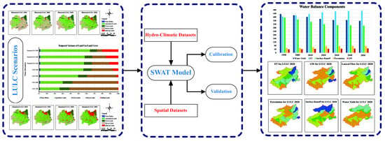
2.3. Methodological Framework

The primary goal of the research is to estimate the implications of LU/LC changes on water balance under historical and projected scenarios, and the detailed methodology employed for this research is given in Figure 3. This study is structured into four major components: (a) To perform supervised classification of satellite imagery for historical LU/LC, (b) To project LU/LC, (c) To set up a hydrological model, (d) To quantify water balance under LU/LC scenarios.

2.4. Cellular Automata Markov Chain Model (CA-MCM)

The Cellular Automata Markov Chain Model (CA-MCM) is a widely accepted LU/LC change modeling algorithm for projecting spatiotemporal changes. The CA-MCM combines Cellular Automata (CA, a spatial model) and the Markov Chain (MCM, a quantitative temporal model) to project LU/LC change trends and characteristics over time. The rationale for integrating the models is that the MCM describes the likelihood of cells changing from one form to another but does not provide spatial distribution. Therefore, to distribute the projected changes spatially, the MCM is hybridized with CA [20,23,24].

MCM is a stochastic model that utilizes two historical LU/LC maps, which are the main inputs for determining the transition area matrix and transition probabilities matrix [49]. For instance, it will provide information on how many cells are likely to transform from one LU/LC class to another based on a transition probability matrix [22,50]. MCM is based on Bayes’ Equation (1) to project LU/LC change, and P is determined using Equation (2):

$${\mathrm{S}}_{\left(\mathrm{t}+1\right)}={\mathrm{P}}_{\mathrm{mn}}\times {\mathrm{S}}_{\left(\mathrm{t}\right)}$$

(1)

$$\mathrm{P} =\Vert \begin{array}{ccccc}{\mathrm{P}}_{11}& {\mathrm{P}}_{12}& {\mathrm{P}}_{13}& \dots & {\mathrm{P}}_{1\mathrm{n}}\\ {\mathrm{P}}_{21}& {\mathrm{P}}_{22}& {\mathrm{P}}_{23}& \dots & {\mathrm{P}}_{2\mathrm{n}}\\ {\mathrm{P}}_{31}& {\mathrm{P}}_{32}& {\mathrm{P}}_{33}& \dots & {\mathrm{P}}_{3\mathrm{n}}\\ ⋮& ⋮& ⋮& ⋮& ⋮\\ {\mathrm{P}}_{\mathrm{m}1}& {\mathrm{P}}_{\mathrm{m}2}& {\mathrm{P}}_{\mathrm{m}3}& \dots & {\mathrm{P}}_{\mathrm{mn}}\end{array}\Vert$$

(2)

where {0 ≤ P_mn ≤ 1 and $\sum _{m,n=1}^j\left({\mathrm{P}}_{\mathrm{mn}}\right)=1 \left(m,n=1,2,3,\dots ,j\right)\}$.

MCM is unable to recognize spatial variability in LU/LC due to a spatial constraint. So, by coupling MCM with CA, spatial and temporal LU/LC changes can be simulated. CA can be expressed as Equation (3):

$${\mathrm{S}}_{\left(\mathrm{t},\mathrm{t}+1\right)}=\mathrm{f} \{{\mathrm{P}}_{\left(\mathrm{t}\right)},\mathrm{N}\}$$

(3)

where S_t and S_t+1 are the LU/LC condition at the time of t and t + 1, respectively; P is the transition probability matrix, j is the number of LU/LC classes, N is the cellular field, and f is the transformation rule of cellular states [13,22,51].

2.5. SWAT Model

SWAT is a physically based, continuous time series, a semi-distributed hydrological model that functions on sub-daily/daily time steps. It was devised to determine the influence of land management strategies on water, sediment, and agricultural chemical yields over extended time periods in a large-scale, complex watershed with heterogeneous soil, slope, and LU/LC scenarios [2,34,52]. The SWAT model simulates a hydrological cycle using the water budget Equation (4):

$${\mathrm{SW}}_{\mathrm{f}}={\mathrm{SW}}_{\mathrm{i}}+{\displaystyle \sum }_{\mathrm{n}=1}^{\mathrm{t}}\left({\mathrm{R}}_{\mathrm{day}}-{\mathrm{Q}}_{\mathrm{surface}}-{\mathrm{W}}_{\mathrm{seep}}-{\mathrm{E}}_{\mathrm{ET}}-{\mathrm{Q}}_{\mathrm{gw}}\right)$$

(4)

The SWAT model employs the Soil Conservation Service curve number (SCS-CN) to characterize the surface runoff [52], which can be defined as Equation (5):

$${\mathrm{Q}}_{\mathrm{surface}}=\frac{{\left({\mathrm{R}}_{\mathrm{day}}-{\mathrm{I}}_{\mathrm{a}}\right)}^2}{{\mathrm{R}}_{\mathrm{day}}-{\mathrm{I}}_{\mathrm{a}}+\mathrm{S}},\hspace{1em} {\mathrm{I}}_{\mathrm{a}}=\lambda S$$

(5)

where SW_f is the final water content of the soil, SW_i is the initial soil water content, t is time (days), R_day, Q_surface, E_ET, W_seep, Q_gw, I_a, and S are the daily amount of precipitation, surface flow, evapotranspiration, percolation, return flow, initial abstraction, and the retention parameter after runoff begins, respectively; all the parameters are measured in mm of H₂O. When I_a is taken to be 0.2S, Equation (6) becomes:

$${\mathrm{Q}}_{\mathrm{surface}}=\frac{{\left({\mathrm{R}}_{\mathrm{day}}-0.2\mathrm{S}\right)}^2}{{\mathrm{R}}_{\mathrm{day}}+0.8\mathrm{S}},\hspace{1em} \mathrm{for} \mathrm{P}>0 \mathrm{else} \mathrm{Q}=0$$

(6)

The retention parameter fluctuates geo-spatially owing to the changes in LU/LC, soil, slope, and soil water content, and it may be computed using Equation (7) [31,53,54].

$$\mathrm{S}=\frac{25,400}{\mathrm{CN}}-254$$

(7)

Evapotranspiration of the basin is evaluated using the Penman–Monteith method, which can be defined as Equation (8).

$$\mathsf{\lambda }\ast \mathrm{ET}=\frac{\Delta \left({\mathrm{R}}_{\mathrm{n}}-\mathrm{G}\right)+{\mathsf{\rho }}_{\mathrm{a}}{\mathrm{c}}_{\mathrm{p}}\ast \left(\frac{{\mathrm{e}}_{\mathrm{s}}-{\mathrm{e}}_{\mathrm{a}}}{{\mathrm{r}}_{\mathrm{a}}}\right)}{\Delta +\mathsf{\gamma }\ast \left(1+\frac{{\mathrm{e}}_{\mathrm{s}}}{{\mathrm{r}}_{\mathrm{a}}}\right)}$$

(8)

where R_n, G, e_s − e_a, ρ_a, r_s, r_a, c_p, and g are the lateral flow, transmission losses, net radiation, soil heat flux, air vapor pressure deficit, mean air density, surface resistance, aerodynamic resistance, the specific heat of air, and psychrometric constant, respectively.

2.6. Evaluation of Historical Land Use/Land Cover

The assessment of LU/LC was accomplished by employing four satellite imagery, three (3) from Landsat with a spatial resolution of 30 m and one (1) from Sentinel with a spatial resolution of 10 m, namely, Landsat-5 TM 1990, Landsat-7 ETM+ 2000, Landsat-7 ETM+ 2010, and Sentinel-2A 2020, respectively (Table S1). Landsat 7 ETM+ had scan line errors which were collected after 31 May 2003 due to a malfunction of the scan line corrector (SLC). Firstly, these scan line errors were corrected using the Landsat tool. After this operation, the next step was to perform the supervised classification, which was executed using Imagine ERDAS software. For this purpose, more than 700 training samples were acquired to create signature files that were further used to execute supervised classification based on the Maximum Likelihood Classification (MLC) algorithm [34,35]. After successful classification, the accuracy assessment of the classified images was performed using the ground truth data. For this purpose, 100 points for each LU/LC type were taken using Google Earth maps and satellite imageries. After ground truthing, Imagine ERDAS automatically calculated the kappa coefficient, overall, producer’s and user’s accuracy.

2.7. Land Use/Land Cover Projection

CA-MCM is available in MOLUSCE (Modules for Land Use Change Simulations), an extension of QGIS, and is a comprehensive model that projects the trends and geospatial configuration of LU/LC classes based upon historical LU/LC thematic maps, transition probability matrices, and suitability matrices [34,55]. Before proceeding towards the projection of LU/LC, inputs were required. The first input was the creation of three discrete LU/LC classified maps, two maps for the preparation of the transition probability matrix, and one map to validate the model. The other input was the driving parameters, which include the spatial and socio-economic factors (Table S4). Several parameters can control the growth in each LU/LC class, and these parameters can interact and establish an intricate relationship. Thus, major driving parameters such as topography, aspect, slope, Euclidean distance from roads, Euclidean distance from railways, Euclidean distance from water bodies, gross domestic product (GDP), and population density (Figure S1) were chosen depending on their availability and impact on LU/LC changes [14,24,56]. These driving factors were used to prepare the suitability matrix. The classified LU/LC maps of 2000 and 2010 were employed to generate a transition probability matrix and driving parameters to create a suitability matrix. MLP-ANN algorithm used these matrices to project the LU/LC map of 2020. This projected map was validated with a supervised classified LU/LC 2020 map [14,57]. After successful validation, the trained model was used to project LU/LC to 2030, 2040, and 2050.

2.8. Setup, Sensitivity Analysis, Calibration and Validation of SWAT

A SWAT model was employed to simulate the implications of the historical and projected LU/LC change scenarios on water balance components in the Potohar Plateau. The Arc-SWAT 2012 model delineated the whole region into three major river basins, namely Soan, Haro, and Kanshi. These basins were divided into multiple sub-basins by choosing a threshold value of 5005 hectares. Since these sub-basins had heterogeneity, they were further segmented into hydrologic response units (HRUs) associated with distinct sets of topography, soil, and LU/LC class with the threshold value of 10%, 20%, and 10%, respectively, as put forth by Kiprotich [7]. These HRUs were homogeneous geospatial units with identical hydrological and geomorphological characteristics. In our case, this region had 3 river basins, 57 sub-basins, and 486 HRUs for the baseline model. The model performed a simulation using high-resolution gridded climatic data such as precipitation, and minimum and maximum temperature for a span of 29 years (1991–2019), encapsulating a spin-up period of an initial three years [28,58,59,60].

The SWAT model was refined by coupling it with SWAT Calibration and Uncertainty Programs (SWAT-CUP). The SUFI-2 algorithm enables parameterization using sensitivity analysis, calibration, and validation [61,62]. In order to carry out this operation, available observed data was divided into three-time windows, with the middle time window used for model calibration and rest two windows used for backward and forward validations. These windows were defined such that the monthly average and standard deviation were nearly equal for all the windows.

Based on past research on similar catchments, thirty-eight of the most influential parameters were chosen for sensitivity analysis. Global Sensitivity Analysis (GSA) was employed to perform sensitivity analysis. The sensitivity of the parameters was determined using a multiple regression approach that regresses Latin hypercube-generated parameters against an objective function. Due to the diverse number of parameters, the calibration process becomes complex and computationally extensive. So, to reduce the number of parameters, local sensitivity analysis was also performed, which not only reduced the number of parameters but also provided upper and lower bounds for an expeditious calibration process [63,64]. In order to analyze the SWAT performance during the simulation, we applied four statistical performance indicators given in

Table 2. List of employed statistical parameters.

Coefficient	Formula	Performance Rating
R2: Coefficient of determination	${\mathrm{R}}^2=\frac{{\left[{{\displaystyle \sum }}_{\mathrm{i}=1}^{\mathrm{n}}\left({\mathrm{Q}}_{\mathrm{obs},\mathrm{i}}-\overline{{\mathrm{Q}}_{\mathrm{obs}}}\right)\left({\mathrm{Q}}_{\mathrm{sim},\mathrm{i}}-\overline{{\mathrm{Q}}_{\mathrm{sim}}}\right)\right]}^2}{{{\displaystyle \sum }}_{\mathrm{i}=1}^{\mathrm{n}}{\left({\mathrm{Q}}_{\mathrm{obs},\mathrm{i}}-\overline{{\mathrm{Q}}_{\mathrm{obs}}}\right)}^2{{\displaystyle \sum }}_{\mathrm{i}=1}^{\mathrm{n}}{\left({\mathrm{Q}}_{\mathrm{sim},\mathrm{i}}-\overline{{\mathrm{Q}}_{\mathrm{sim}}}\right)}^2}$	0 ≤ R2 ≤ 1 >0.5 Satisfactory >0.65 Good
NSE: Nash–Sutcliffe Efficiency	$\mathrm{NSE}=1-\frac{{{\displaystyle \sum }}_{\mathrm{i}=1}^{\mathrm{n}}{\left({\mathrm{Q}}_{\mathrm{obs}}-{\mathrm{Q}}_{\mathrm{sim}}\right)}^2}{{{\displaystyle \sum }}_{\mathrm{i}=1}^{\mathrm{n}}{\left({\mathrm{Q}}_{\mathrm{obs},\mathrm{i}}-\overline{{\mathrm{Q}}_{\mathrm{obs}}}\right)}^2}$	0 ≤ NSE ≤ 1 >0.5 Satisfactory >0.65 Good
KGE: Kling–Gupta efficiency	$\mathrm{KGE}=1-\sqrt{{\left(\mathrm{r}-1\right)}^2+{\left(\mathsf{\alpha }-1\right)}^2+{\left(\mathsf{\beta }-1\right)}^2}$	0 ≤ KGE ≤ 1 >0.5 Satisfactory >0.65 Good
PBIAS: Percent bias	$\mathrm{PBIAS}=100\times \frac{{{\displaystyle \sum }}_{\mathrm{i}=1}^{\mathrm{n}}{({\mathrm{Q}}_{\mathrm{obs}}-{\mathrm{Q}}_{\mathrm{sim}})}_{\mathrm{i}}}{{{\displaystyle \sum }}_{\mathrm{i}=1}^{\mathrm{n}}{\mathrm{Q}}_{\mathrm{obs},\mathrm{i}}}$	−∞ ≤ PBIAS ≤ +∞ <±25 Satisfactory <±15 Good

[52,65].

3. Results

3.1. Spatio-temporal Changes in Historical LU/LC

The LU/LC maps were classified into five classes, i.e., water bodies, agricultural lands, forest lands, barren lands, and built-up lands. Principally, it was conceived that there was an escalating anthropogenic biome in the region owing to the infrastructural development and high land-intensive agriculture, and abatement of barren and forest lands, resulting in a major loss of natural cover. The spatiotemporal distribution of LU/LC change in the Plateau is depicted in Figure 4. It demonstrates that built-up lands were drastically increased in the northern areas by transforming agricultural, forest, and barren lands into non-porous lands between 1990 and 2020 (Figure 5). Concurrently, barren land was converted to machine-intensive agricultural land in the central and southern areas. A similar scenario prevailed in the subsequent decades, with the sprawl of unregulated settlements and agricultural activities at the detriment of barren and forest lands.

The historical LU/LC change (

Table 3. Historical LU/LC composition in the Plateau.

LU/LC	Classified 1990		Classified 2000		Classified 2010		Classified 2020
	Km2	%	Km2	%	Km2	%	Km2	%
Water Bodies	252.04	1.08	316.56	1.36	324.59	1.40	338.76	1.46
Agriculture Lands	5790.60	24.91	6631.58	28.58	11,102.87	47.85	12,655.54	54.43
Forest Lands	2859.59	12.30	2786.42	12.01	2585.14	11.14	2478.51	10.66
Barren Lands	14,086.34	60.59	13,159.87	56.71	8637.84	37.23	6190.87	26.63
Built-up Lands	260.79	1.12	309.55	1.33	553.63	2.39	1585.67	6.82

) was dominated by the change in a barren land with a total loss of 7895.47 km², followed by urban and agriculture. Agricultural land and built-up land exhibited an increasing trend gaining 6864.94 km² and 1585.67 km², respectively, while water changed the least. The highest decline in barren lands was primarily owing to the proliferation of agricultural and built-up lands. The agricultural lands were expanded to fulfill the agrarian needs and generate livelihood for the increasing population, while the built-up lands were expanded to accommodate migration from rural communities to major urban centers.

However, the LU/LC change is trivial compared to the Plateau’s total geographical area. This signifies that the LU/LC change has been more substantial at the sub-basin level than at the Plateau level. At the Plateau level, positive LU/LC changes in one class have been counterbalanced by negative LU/LC changes in another class. For example, an increase in agricultural activity has been observed in central and downstream areas, simultaneously, the transition of agricultural land to built-up land in upstream areas led to a decline in agricultural land within the Plateau. The findings of this research are congruent with those of others conducted on and around the Plateau. For instance, in the Potohar Plateau, [37,38] concluded that there was a dramatic increase in agricultural and infrastructural development. The authors of [57] also summarized that the built-up land are increasing, which is causing the loss of vegetation cover in the northern part of the region.

3.2. Accuracy Assessment of Supervised Classified LU/LC Maps

Accuracy assessment was used to determine the reliability of classified images. In this regard, a confusion matrix was employed to determine the correctness of the classified image. Randomly selected sampling points were analyzed on the classified maps from Google Earth maps and mosaicked satellite imagery as a reference. Around 500 ground truthing points for each classified image, with 100 sampling points for each class, were selected to validate images from 1990, 2000, 2010, and 2020. The results (Table S3) exhibit that the average kappa coefficient and overall accuracy for 1990, 2000, 2010, and 2020 maps were 0.79, 0.81, 0.82, and 0.84; 83.8%, 85.2%, 85.88%, and 87.8%, respectively. The producer’s accuracy ranged between 75% and 94%, while the user’s accuracy ranged between 79% and 97%. According to Monserud and Landis [66,67], a Kappa coefficient above 0.75 is an acceptable indicator of the classified image. Therefore, the outcome of the assessment demonstrated that the classified image and ground truths were in good agreement.

3.3. LU/LC Projections

LU/LC maps of 2000 and 2010 functioned as observed data for training the CA-MCM, whereas the LU/LC map of 2020 was utilized to evaluate the reliability of the projected map for 2020. A comparative analysis of classified and projected LU/LC maps for 2020 was conducted. The pictorial comparison demonstrates that the CA-MCM was an effective LU/LC projection tool for the Potohar Plateau (Figure 4). An assessment of conformity between classified and projected maps for 2020 was performed to ascertain the adaptability of the deployed model to reliably simulate the distribution of LU/LC changes (Table S7). The Kappa coefficient (K) was determined to comprehend the resemblance between the classified and projected LU/LC maps for 2020. Since all the K statistics (K_overall = 0.77, K_historical = 0.79, and K_local = 0.82) have been above the value of 0.75 [63,64], the CA-MCM trained for LU/LC projection was deemed to be acceptable.

Furthermore, since the hydrological model was taken into account to estimate the implications of LU/LC change on the water balance of the study area, a comparison between the simulations performed using the classified LU/LC 2020 map, and the CA-MCM projected LU/LC 2020 map (Figure S4) was necessary. The graphical analysis reveals that the flow regime simulated by the SWAT model at the river basins changed minimally for the two employed LU/LC maps (Figure S3), restating the good match between the classified and simulated LU/LC maps. The trained CA-MCM was then utilized to project LU/LC maps for 2030, 2040, and 2050 (

Table 4. Future projected LU/LC composition in the Plateau.

LU/LC	Projected 2020		Projected 2030		Projected 2040		Projected 2050
	Km2	%	Km2	%	Km2	%	Km2	%
Water Bodies	334.69	1.46	353.53	1.52	350.57	1.51	348.44	1.50
Agriculture Lands	12,439.41	54.43	12,831.91	55.19	13,040.56	56.09	14,586.03	62.74
Forest Lands	2335.59	10.66	2314.06	9.95	2189.18	9.42	2054.69	8.84
Barren Lands	6289.47	26.63	5119.34	22.02	4043.06	17.39	1522.11	6.55
Built-up Lands	1800.17	6.82	2630.50	11.31	3627.24	15.60	4738.08	20.38

).

The LU/LC change detection of the Potohar Plateau indicates that agricultural lands hold the dominant portion of the area (Figure 4). From the analysis, it is clear that the study area has assimilated significant LU/LC change, and the dominant LU/LC change has occurred in the expansion of built-up and agricultural lands. Additionally, LU/LC change has been occurring at the expense of a reduction in barren and forest lands (Figure S2).

3.4. Hydrological Model Calibration and Validation

The initial SWAT model setup utilizing default parameter ranges was unable to successfully simulate the flow regime at all hydrometric gauges because the base flow and peak flow were overestimated. As a result, parameter calibration was required to precisely model the hydrologic regime. A global sensitivity analysis (GSA) for the simulated flow was undertaken using a monthly hydrometric flow to recognize the most sensitive parameters which affect model response. Incipiently soil, groundwater, evapotranspiration, surface runoff, and geomorphology parameters were considered, and 29 parameters were recognized as sensitive parameters. The greater the absolute value of the t-stat and the lower the p-value, the more sensitive a parameter, and the sensitivity ranks of parameters after GSA are shown in Table S5. Subsequently, the calibration was performed incorporating 29 parameters [28,63], which was laborious and computationally intensive. Therefore, local sensitivity analysis (LSA) was also performed, reducing the number of parameters to 22 and providing upper and lower bounds for swift calibration (Table S6). The model was calibrated to flow series from 1998 to 2003. The calibrated and validated parameter values were integrated into the SWAT database to estimate the implications of LU/LC on the water balance.

The SWAT model performed well during calibration (1998–2003) and validation (1994–1997 and 2004–2007) windows. According to the visual analysis of the stream flows (Figure 5 and Figures S5 and S6) and statistical evaluation of the model using R², NSE, KGE, and PBIAS with reference to criteria defined by Moriasi [65], all hydrometric gauges demonstrated good or very good performance during calibration and validation windows, and the statistical performance indices are shown in

Table 5. Statistical performance of model during calibration and validation windows.

River Basin	Calibration				Backward Validation				Forward Validation
	R2	NSE	KGE	PBIAS	R2	NSE	KGE	PBIAS	R2	NSE	KGE	PBIAS
Soan	0.81	0.79	0.77	9.8	0.78	0.76	0.75	−12.9	0.78	0.76	0.76	−17.8
Haro	0.80	0.77	0.78	8.7	0.76	0.74	0.76	8.7	0.76	0.76	0.77	12.7
Kanshi	0.77	0.79	0.73	19.7	0.77	0.74	0.74	14.7	0.75	0.74	0.73	10.6

. Furthermore, R-factor and p-value statistics criteria are governed by Karim Abbaspour’s [61] model exhibits a good agreement with the calibration and validations. Overall, the performance rating indices computed during the calibration and validation windows confirmed that the model performed quite well [27,68], which suggests that it has the potential to model the implications of LU/LC changes on the hydrological regime.

3.5. Plausible Impacts of LU/LC Changes on Hydrological Regime

Four supervised classified LU/LC maps of the Potohar Plateau (1990, 2000, 2010, and 2020) and three future projected LU/LC maps (2030, 2040, and 2050) were deployed in the calibrated SWAT model under the assumption that the climate was immutable. The impact of LU/LC alterations on the hydrological responses was assessed using a baseline model over the span of 29 years (1991–2019), including a three-year spin-up period (1991–1993) and with varied LU/LC maps, for instance, LU/LC 2000, LU/LC 2010, LU/LC 2020, LU/LC 2030, LU/LC 2040, and LU/LC 2050.

The hydrological regime was investigated in terms of how hydrological processes respond to evapotranspiration, water yield, surface, and sub-surface flows, as exhibited in

Table 6. Mean annual water balance components of the river basins.

Components (mm)	1990	2000	2010	2020	2030	2040	2050
Precipitation	845.80	845.80	845.80	845.80	845.80	845.80	845.80
Surface Runoff	394.09	372.96	348.94	319.82	309.34	307.98	303.33
Evapotranspiration	406.65	419.67	433.96	452.66	464.60	468.66	471.80
Percolation	52.83	54.32	63.55	72.60	73.22	74.94	76.08
Groundwater Flow	38.43	39.45	42.71	44.35	44.73	46.61	48.02
Return Flow	5.14	6.59	6.94	7.04	7.15	7.32	8.61
Lateral Flow	8.63	9.43	9.46	9.70	10.03	10.09	10.16
Water Yield	432.87	419.37	402.11	378.84	366.61	366.27	357.95

. As a consequence of the anticipated drastic transformation of LU/LC from 1990 to 2020, mean annual evapotranspiration (+11%) and groundwater flow (+15%) tend to increase, while mean annual surface flow (−19%) and total water yield (−12%) decreased. Nevertheless, the rate of increase and decrease is proportional to the rate of change in LU/LC. In general, the exacerbating ramifications of the LU/LC changes are accompanied by increased agricultural and built-up lands in conjunction with decreased forest and barren lands.

According to the LU/LC scenarios, agricultural lands are anticipated to increase from 24.91% to 62.74%, while built-up lands are expected to increase from 1.12% to 20.38%, leading to an increase in evapotranspiration (+15.54%) and a decrease in surface runoff (−24%), as shown in

Table 7. Comparison between water balance components under LU/LC scenarios.

Components (mm)	Baseline Scenario (1990)	Recent Scenario (2020)	Mid-Century Scenario (2050)	Baseline to Recent (%)	Recent to Mid-Century (%)
Surface Runoff	394.09	319.82	303.33	−74.28 (−18.85%)	−16.49 (−5.15%)
Evapotranspiration	406.65	452.66	471.80	46.01 (11.31%)	19.14 (4.23%)
Water Yield	432.87	378.84	357.95	−54.03 (−12.48%)	−20.90 (−5.52%) *

* The number in parentheses indicates a percent change.

[12,51]. In the research area, from 1990 to 2050, agricultural expansion (+37.84%) dominated infrastructural development (+19.26%). Therefore, it may neutralize the implications of built-up lands on hydrological components, decreasing surface flow. The expansion of machine-intensive agriculture with the loss of barren land may be the cause of the flow reduction.

4. Discussion

The integration of LU/LC with the SWAT model can enhance the performance of the model in simulating the processes happening in the basins. In this study, the impacts of LU/LC changes on water balance were estimated for the Potohar Plateau. In this context, supervised classification was performed using ERDAS Imagine for the satellite imageries for the years 1990, 2000, 2010, and 2020. Subsequently, the future of LU/LC was projected using CA-MCM for the years 2030, 2040, and 2050. After that, the SWAT model was set up for the base year and then calibrated and validated to enhance its efficiency of the model. A SWAT model with optimized parameters was utilized to quantify the plausible impact of LU/LC changes in the water balance on the sub-basin level.

The analysis of LU/LC maps of 1990, 2000, 2010, 2020, 2030, 2040, and 2050 revealed that an increase in agricultural and built-up areas from 24.91% to 54.43% and 1.12% to 6.82% and likely to be increased to 62.74% and 20.38%, respectively, in the mid-century due to an increase in demographic and socio-economic growth. The LU/LC analysis also showed that a decrease in forest and barren lands from 12.30% to 10.66% and 60.59% to 26.63% are likely to be increased to 8.84% and 6.55%, respectively, as presented in Table 3 and Table 4. The authors of [37] showed that there is an increase in agricultural and built-up areas from 11% to 29% and 6% to 11%, respectively, while forest and barren areas reduced from 69% to 43% and 16% to 10%, respectively, in the Simly watershed. The researchers of [69] also showed that there is an increase in agricultural and built-up areas from 33.44% to 63.1% and 1.77% to 5.78%, respectively, while forest and waste lands reduced from 29.81% to 11.32% and 9.27% to 2%, respectively, in the Narmada watershed. This built-up area and forest shift are more prominent in the northern regions and urban centers, especially in the twin cities. Similarly, an augmentation in agriculture and the associated loss of barren land in the central and southern regions of the Plateau as shown in Figure 4. An analysis from the authors of [38] showed similar patterns in the Potohar Plateau, confirming that there is an increase in agriculture in the central and south-eastern regions and increased urbanization in north-western and developed areas. The findings of other studies in the Astore basin, Pakistan [21], Bogota basin, Colombia [3], Ganga basin, India [4], and Geba catchment, Ethiopia [70] are also in agreement with this study.

Hydrological models are crucial for evaluating the implications of LU/LC changes on water balance. The model is selected in conformity with the problem complexity, data availability, computing cost, and model robustness [12,27,68]. A comparison of different hydrological models was conducted on those models that are suitable for evaluating the influence of LU/LCC on the water balance. The SWAT model was the best for the punctilious modeling of LU/LC changes on the flow regime. The SWAT model was also recommended since it had been commonly employed in large-scale modeling and simulations to evaluate the plausible ramifications of land management practices and LU/LC changes on the hydrologic components [52,62]. In this study, the SWAT model setup for the baseline scenario was calibrated for the period 1998 to 2003, backward validated from 1994–1997, and forward validated from 2004–2007, as this approach was followed by Dahri et al., 2021. The result of statistical indices, i.e., R², NSE, KGE, and PBIAS for calibration and validation windows ranged between 0.75–0.81, 0.74–0.79, 0.73–0.78, and −17.8–+14.7%, respectively. Overall, the performance rating indices computed during calibration, and validation windows revealed that the model performed quite well [52,62,65], which suggests that it has the potential to model the implications of LU/LC changes on the hydrological regime.

The quantitative analysis of water balance components revealed that the decrease in surface runoff and water yield from 394.09 mm to 319.82 mm and 432.87 mm to 432.87 mm are likely to be increased to 303.33 mm and 357.95 mm, respectively, in mid-century due to LU/LC changes [4,71]. It also showed an increase in evapotranspiration, percolation, groundwater flow, and lateral flow from 406.65 mm to 452.66 mm, 52.83 mm to 72.60 mm, 38.43 mm to 44.35 mm, and 8.63 mm to 9.70 mm, and are likely to be increased to 471.80 mm, 76.08 mm, 48.02 mm, and 10.16 mm, respectively, as presented in Table 6 [51,72]. The potential of the model to simulate the geospatial distribution of hydrological components provides a substantial contribution to sustainable watershed management. At HRU and sub-basin level, the spatial distribution of hydrological components, namely evapotranspiration, water yield, surface runoff, percolation, lateral flow, and groundwater flow, have been computed as shown in Figure 6, Figure 7 and Figures S7–S10. Evapotranspiration of the Plateau was lesser in the northern parts and higher in the central and southern parts (Figure 7). Conversely, besides climatic and orographic variations, surface runoff, and water yield had a high concentration in the northern region due to the transformation of agricultural and forest lands into built-up land, while a lower concentration was found in the central and southern regions due to the conversion of barren land into agricultural land (Figure 6 and Figure S7).

The decreased surface runoff may be accompanied by an increase in evapotranspiration, percolation, lateral flow, and decreased runoff, signifying the augmentation of soil water storage. Groundwater flow varied comparatively less in the proximity of the northern districts and higher in the southern districts. An increase in groundwater flow was simulated on plain terrain, and there was relatively no change in the hilly terrain (Figure S8). Unlike surface runoff, the lateral flow was higher in plain terrain and low infiltration areas. The southern region was found to contribute significant lateral flow to streamflow. Seasonal streamflow variability was also evaluated for the wet and dry seasons (Figure S11). The streamflow was slightly increased in the wet season and decreased in the dry season under the LU/LC scenarios. This increase and decrease in flow might be due to increased urbanization and agricultural activities, respectively. However, it was concluded from the quantitative outputs of the SWAT model that the implications of LU/LC changes were more pronounced at the sub-basin level than at the basin level [4,64,73,74]. The findings are in agreement with other studies conducted in watersheds around the globe. For instance, [72] in the Nam Rom catchment, Vietnam concluded that LU/LC changes have reduced surface runoff and increased evapotranspiration. The authors of [51] in the Beiluo river basin on the Loess Plateau of China found that on an annual scale, surface runoff and water yield may gradually decrease, but evapotranspiration may increase. The authors of [69] also showed a decline of surface runoff and water yield but higher ET due to the presence of more vegetation and forest areas between 1990–2050 in the Narmada river basin, India, which was attributed to the LU/LCC of the catchment.

Despite the fact that the Soan, Haro, and Kanshi river basins encompass 78% of the Potohar Plateau, this still does not meticulously characterize the Plateau, as it constitutes three other river basins. Further studies on the other river basins are required to completely comprehend the dynamics of water balance components in the Plateau. Overall, the SWAT model simulated the flow regimes and water balance components efficiently. However, the accuracy of the simulations is constrained by the coarse resolution of soil data, uncertainties in hydrometric data [75], unavailability of reservoirs data (small dams), evapotranspiration data, and groundwater flow data for the calibration and validation of the model, these should be incorporated in subsequent studies. Moreover, climate change impacts should also be studied in conjunction with LU/LC changes to develop rational strategies for sustainable water management.

5. Conclusions

The enclosed research executed a methodical framework that comprised LU/LC scenarios, hydrological modeling, and quantification of hydrological components alteration in the Potohar Plateau, which were attributed to the effects of human-induced LU/LC changes. Seven distinct LU/LC scenarios were accomplished and evaluated by means of the hydrological SWAT model. Furthermore, the outcomes of each scenario were compared to those of the baseline scenario. According to historical LU/LC maps from 1990 to 2020, anthropogenic pressure increased agriculture and built-up lands by 29.52 and 7.7%, respectively, while barren and forest lands decreased by 33.96 and 1.64%, respectively. LU/LC projections for 2030, 2040, and 2050 were simulated using CA-MCM, which showed an increase in agricultural and built-up lands with decreased barren and forest lands. Among all LU/LC scenarios from 1990 to 2050, it is anticipated that the agricultural and built-up lands will have the greatest proliferation.

The hydrological regime was modeled through the SWAT model, which was then compared to observed hydrometric flows. The SWAT model was calibrated and validated by simulating flow time series from 1994 to 2007. After calibration and validations, the obtained results of the four most recommended coefficients R², NSE, KGE, and PBIAS for calibration ranged between 0.77–0.81, 0.77–0.79, 0.73–0.78, and +9.8–+19.7%, respectively, while for forward and backward validation, values ranged between 0.75–0.78, 0.74–0.76, 0.73–0.77, and −17.8–+14.7%, respectively. The result of statistical indices and visualization of streamflow yields a good degree of agreement between the simulated and observed flow regimes, which indicates that the calibrated model, in conjunction with optimized parameters, has the ability to simulate the water balance under LU/LC scenarios.

A distinct outcome of this study is that the transformation in intrinsic water balance and flow regime is substantially sensitive to alteration in LU/LC. The analysis signifies that the influence of LU/LC change has been diverse for peculiar river basins and more prominent at the sub-basin level. The anticipated results indicate that LU/LC attributes to dramatic decrease of surface runoff and water yield by 19% and 12%, respectively, which is expected to exacerbate. Conversely, there is an increase in groundwater flow, lateral flow, and evapotranspiration of 15%, 12%, and 11%, respectively, largely due to the transformation of barren land into agricultural land.

The findings of this study lead to a greater comprehension of the plausible effects of LU/LC changes on water balance in the Potohar Plateau, which will substantially aid decision-makers in planning and executing potential adaptation strategies for watersheds under changing LU/LC scenarios. Moreover, the methodological framework of this research can be useful for any other watershed to evaluate the effects of anthropogenic biomes on the hydrological regime.

References

1. Idrissou, M.; Diekkrüger, B.; Tischbein, B.; de Hipt, F.O.; Näschen, K.; Poméon, T.; Yira, Y.; Ibrahim, B. Modeling the Impact of Climate and Land Use/Land Cover Change on Water Availability in an Inland Valley Catchment in Burkina Faso. Hydrology 2022, 9, 12. [Google Scholar] [CrossRef]
2. Ha, L.T.; Bastiaanssen, W.G.M.; Van Griensven, A.; Van Dijk, A.I.J.M.; Senay, G.B. Calibration of Spatially Distributed Hydrological Processes and Model Parameters in SWAT Using Remote Sensing Data and an Auto-Calibration Procedure: A Case Study in a Vietnamese River Basin. Water 2018, 10, 212. [Google Scholar] [CrossRef] [Green Version]
3. Clerici, N.; Cote-Navarro, F.; Escobedo, F.J.; Rubiano, K.; Villegas, J.C. Spatio-temporal and cumulative effects of land use-land cover and climate change on two ecosystem services in the Colombian Andes. Sci. Total Environ. 2019, 685, 1181–1192. [Google Scholar] [CrossRef]
4. Anand, J.; Gosain, A.; Khosa, R. Prediction of land use changes based on Land Change Modeler and attribution of changes in the water balance of Ganga basin to land use change using the SWAT model. Sci. Total Environ. 2018, 644, 503–519. [Google Scholar] [CrossRef]
5. Ellis, E.C.; Beusen, A.H.; Goldewijk, K.K. Anthropogenic Biomes: 10,000 BCE to 2015 CE. Land 2020, 9, 129. [Google Scholar] [CrossRef]
6. Verburg, P.H.; Neumann, K.; Nol, L. Challenges in using land use and land cover data for global change studies. Glob. Chang. Biol. 2011, 17, 974–989. [Google Scholar] [CrossRef] [Green Version]
7. Kiprotich, P.; Wei, X.; Zhang, Z.; Ngigi, T.; Qiu, F.; Wang, L. Assessing the Impact of Land Use and Climate Change on Surface Runoff Response Using Gridded Observations and SWAT+. Hydrology 2021, 8, 48. [Google Scholar] [CrossRef]
8. Kim, J.; Choi, J.; Choi, C.; Park, S. Impacts of changes in climate and land use/land cover under IPCC RCP scenarios on streamflow in the Hoeya River Basin, Korea. Sci. Total Environ. 2013, 452–453, 181–195. [Google Scholar] [CrossRef]
9. Gashaw, T.; Tulu, T.; Argaw, M.; Worqlul, A.W. Modeling the hydrological impacts of land use/land cover changes in the Andassa watershed, Blue Nile Basin, Ethiopia. Sci. Total Environ. 2018, 619–620, 1394–1408. [Google Scholar] [CrossRef] [PubMed]
10. Baker, T.J.; Miller, S.N. Using the Soil and Water Assessment Tool (SWAT) to assess land use impact on water resources in an East African watershed. J. Hydrol. 2013, 486, 100–111. [Google Scholar] [CrossRef]
11. Neupane, R.P.; Kumar, S. Estimating the effects of potential climate and land use changes on hydrologic processes of a large agriculture dominated watershed. J. Hydrol. 2015, 529, 418–429. [Google Scholar] [CrossRef]
12. Chanapathi, T.; Thatikonda, S. Investigating the impact of climate and land-use land cover changes on hydrological predictions over the Krishna river basin under present and future scenarios. Sci. Total Environ. 2020, 721, 137736. [Google Scholar] [CrossRef]
13. Guo, Y.; Fang, G.; Xu, Y.-P.; Tian, X.; Xie, J. Identifying how future climate and land use/cover changes impact streamflow in Xinanjiang Basin, East China. Sci. Total Environ. 2019, 710, 136275. [Google Scholar] [CrossRef]
14. Kamaraj, M.; Rangarajan, S. Predicting the future land use and land cover changes for Bhavani basin, Tamil Nadu, India, using QGIS MOLUSCE plugin. Environ. Sci. Pollut. Res. 2022, 2022, 1–12. [Google Scholar] [CrossRef]
15. Abhishek; Kinouchi, T.; Abolafia-Rosenzweig, R.; Ito, M. Water Budget Closure in the Upper Chao Phraya River Basin, Thailand Using Multisource Data. Remote Sens. 2021, 14, 173. [Google Scholar] [CrossRef]
16. Huntington, T.G. Evidence for intensification of the global water cycle: Review and synthesis. J. Hydrol. 2006, 319, 83–95. [Google Scholar] [CrossRef]
17. Kinouchi, T. Synergetic application of GRACE gravity data, global hydrological model, and in-situ observations to quantify water storage dynamics over Peninsular India during 2002–2017. J. Hydrol. 2021, 596, 126069. [Google Scholar] [CrossRef]
18. Pan, M.; Sahoo, A.K.; Troy, T.J.; Vinukollu, R.K.; Sheffield, J.; Wood, A.E.F. Multisource Estimation of Long-Term Terrestrial Water Budget for Major Global River Basins. J. Clim. 2012, 25, 3191–3206. [Google Scholar] [CrossRef]
19. Abolafia-Rosenzweig, R.; Pan, M.; Zeng, J.; Livneh, B. Remotely sensed ensembles of the terrestrial water budget over major global river basins: An assessment of three closure techniques. Remote Sens. Environ. 2020, 252, 112191. [Google Scholar] [CrossRef]
20. Wang, Q.; Guan, Q.; Lin, J.; Luo, H.; Tan, Z.; Ma, Y. Simulating land use/land cover change in an arid region with the coupling models. Ecol. Indic. 2020, 122, 107231. [Google Scholar] [CrossRef]
21. Haleem, K.; Khan, A.U.; Ahmad, S.; Khan, M.; Khan, F.A.; Khan, W.; Khan, J. Hydrological impacts of climate and land-use change on flow regime variations in upper Indus basin. J. Water Clim. Chang. 2021, 13, 758–770. [Google Scholar] [CrossRef]
22. Leta, M.; Demissie, T.; Tränckner, J. Modeling and Prediction of Land Use Land Cover Change Dynamics Based on Land Change Modeler (LCM) in Nashe Watershed, Upper Blue Nile Basin, Ethiopia. Sustainability 2021, 13, 3740. [Google Scholar] [CrossRef]
23. Wang, Q.; Wang, H. An integrated approach of logistic-MCE-CA-Markov to predict the land use structure and their micro-spatial characteristics analysis in Wuhan metropolitan area, Central China. Environ. Sci. Pollut. Res. 2022, 29, 30030–30053. [Google Scholar] [CrossRef] [PubMed]
24. Huang, H.; Zhou, Y.; Qian, M.; Zeng, Z. Land Use Transition and Driving Forces in Chinese Loess Plateau: A Case Study from Pu County, Shanxi Province. Land 2021, 10, 67. [Google Scholar] [CrossRef]
25. Tariq, A.; Shu, H. CA-Markov Chain Analysis of Seasonal Land Surface Temperature and Land Use Landcover Change Using Optical Multi-Temporal Satellite Data of Faisalabad, Pakistan. Remote Sens. 2020, 12, 3402. [Google Scholar] [CrossRef]
26. Zhao, M.; He, Z.; Du, J.; Chen, L.; Lin, P.; Fang, S. Assessing the effects of ecological engineering on carbon storage by linking the CA-Markov and InVEST models. Ecol. Indic. 2018, 98, 29–38. [Google Scholar] [CrossRef]
27. Rahman, K.U.; Shang, S.; Shahid, M.; Wen, Y. Hydrological evaluation of merged satellite precipitation datasets for streamflow simulation using SWAT: A case study of Potohar Plateau, Pakistan. J. Hydrol. 2020, 587, 125040. [Google Scholar] [CrossRef]
28. Abbaspour, K.C.; Rouholahnejad, E.; Vaghefi, S.; Srinivasan, R.; Yang, H.; Kløve, B. A continental-scale hydrology and water quality model for Europe: Calibration and uncertainty of a high-resolution large-scale SWAT model. J. Hydrol. 2015, 524, 733–752. [Google Scholar] [CrossRef] [Green Version]
29. Singh, L.; Saravanan, S. Simulation of monthly streamflow using the SWAT model of the Ib River watershed, India. J. Hydro-Environ. Res. 2020, 3, 95–105. [Google Scholar] [CrossRef]
30. Narsimlu, B.; Gosain, A.K.; Chahar, B.R. Assessment of Future Climate Change Impacts on Water Resources of Upper Sind River Basin, India Using SWAT Model. Water Resour. Manag. 2013, 27, 3647–3662. [Google Scholar] [CrossRef]
31. Kumar, N.; Singh, S.K.; Singh, V.G.; Dzwairo, B. Investigation of impacts of land use/land cover change on water availability of Tons River Basin, Madhya Pradesh, India. Model. Earth Syst. Environ. 2018, 4, 295–310. [Google Scholar] [CrossRef]
32. Tanksali, A.; Soraganvi, V.S. Assessment of impacts of land use/land cover changes upstream of a dam in a semi-arid watershed using QSWAT. Model. Earth Syst. Environ. 2020, 7, 2391–2406. [Google Scholar] [CrossRef]
33. Tamm, O.; Maasikamäe, S.; Padari, A.; Tamm, T. Modelling the effects of land use and climate change on the water resources in the eastern Baltic Sea region using the SWAT model. CATENA 2018, 167, 78–89. [Google Scholar] [CrossRef]
34. Getachew, B.; Manjunatha, B.; Bhat, H.G. Modeling projected impacts of climate and land use/land cover changes on hydrological responses in the Lake Tana Basin, upper Blue Nile River Basin, Ethiopia. J. Hydrol. 2021, 595, 125974. [Google Scholar] [CrossRef]
35. Nauman, S.; Zulkafli, Z.; Bin Ghazali, A.H.; Yusuf, B. Impact Assessment of Future Climate Change on Streamflows Upstream of Khanpur Dam, Pakistan using Soil and Water Assessment Tool. Water 2019, 11, 1090. [Google Scholar] [CrossRef] [Green Version]
36. Usman, M.; Ndehedehe, C.; Manzanas, R.; Ahmad, B.; Adeyeri, O. Impacts of Climate Change on the Hydrometeorological Characteristics of the Soan River Basin, Pakistan. Atmosphere 2021, 12, 792. [Google Scholar] [CrossRef]
37. Butt, A.; Shabbir, R.; Ahmad, S.S.; Aziz, N. Land use change mapping and analysis using Remote Sensing and GIS: A case study of Simly watershed, Islamabad, Pakistan. Egypt. J. Remote Sens. Space Sci. 2015, 18, 251–259. [Google Scholar] [CrossRef] [Green Version]
38. Tariq, A.; Riaz, I.; Ahmad, Z.; Yang, B.; Amin, M.; Kausar, R.; Andleeb, S.; Farooqi, M.A.; Rafiq, M. Land surface temperature relation with normalized satellite indices for the estimation of spatio-temporal trends in temperature among various land use land cover classes of an arid Potohar region using Landsat data. Environ. Earth Sci. 2019, 79, 40. [Google Scholar] [CrossRef]
39. Waseem Ghani, M.; Arshad, M.; Shabbir, A.; Shakoor, A.; Mehmood, N.; Ahmad, I. Investigation of Potential Water Harvesting Sites at Potohar Using Modeling Approach. Pakistan J. Agric. Sci. 2013, 50, 723–729. [Google Scholar]
40. Khan, M.T.; Shoaib, M.; Hammad, M.; Salahudin, H.; Ahmad, F.; Ahmad, S. Application of Machine Learning Techniques in Rainfall–Runoff Modelling of the Soan River Basin, Pakistan. Water 2021, 13, 3528. [Google Scholar] [CrossRef]
41. Hussain, F.; Nabi, G.; Wu, R.-S. Spatiotemporal Rainfall Distribution of Soan River Basin, Pothwar Region, Pakistan. Adv. Meteorol. 2021, 2021, 6656732. [Google Scholar] [CrossRef]
42. Nusrat, A.; Gabriel, H.F.; e Habiba, U.; Rehman, H.U.; Haider, S.; Ahmad, S.; Shahid, M.; Jamal, S.A.; Ali, J. Plausible Precipitation Trends over the Large River Basins of Pakistan in Twenty First Century. Atmosphere 2022, 13, 190. [Google Scholar] [CrossRef]
43. Final Results (Census-2017)|Pakistan Bureau of Statistics. Available online: https://www.pbs.gov.pk/content/final-results-census-2017 (accessed on 2 August 2022).
44. ALOS PALSAR—ASF. Available online: https://asf.alaska.edu/data-sets/sar-data-sets/alos-palsar/ (accessed on 13 August 2022).
45. USGS.Gov|Science for a Changing World. Available online: https://www.usgs.gov/ (accessed on 13 August 2022).
46. FAO/UNESCO Soil Map of the World|FAO SOILS PORTAL|Food and Agriculture Organization of the United Nations. Available online: https://www.fao.org/soils-portal/data-hub/soil-maps-and-databases/faounesco-soil-map-of-the-world/en/ (accessed on 13 August 2022).
47. Muhammad, W.K.; Shakil, A.; Zakir, H.D.; Zain, S.; Khalil Ahmad, F.K.M.A. Development of High Resolution Daily Gridded Precipitation and Temperature Dataset for Potohar Plateau of Indus Basin. Remote Sens. 2022, in press. [Google Scholar]
48. Water & Power Development Authority. Available online: http://www.wapda.gov.pk/ (accessed on 31 August 2022).
49. Firozjaei, M.K.; Sedighi, A.; Argany, M.; Jelokhani-Niaraki, M.; Arsanjani, J.J. A geographical direction-based approach for capturing the local variation of urban expansion in the application of CA-Markov model. Cities 2019, 93, 120–135. [Google Scholar] [CrossRef]
50. Tadese, S.; Soromessa, T.; Bekele, T. Analysis of the Current and Future Prediction of Land Use/Land Cover Change Using Remote Sensing and the CA-Markov Model in Majang Forest Biosphere Reserves of Gambella, Southwestern Ethiopia. Sci. World J. 2021, 2021, 6685045. [Google Scholar] [CrossRef] [PubMed]
51. Yan, R.; Cai, Y.; Li, C.; Wang, X.; Liu, Q. Hydrological Responses to Climate and Land Use Changes in a Watershed of the Loess Plateau, China. Sustainability 2019, 11, 1443. [Google Scholar] [CrossRef] [Green Version]
52. Arnold, J.G.; Moriasi, D.N.; Gassman, P.W.; Abbaspour, K.C.; White, M.J.; Srinivasan, R.; Santhi, C.; Harmel, R.D.; van Griensven, A.; Van Liew, M.W.; et al. SWAT: Model Use, Calibration, and Validation. Trans. ASABE 2012, 55, 1491–1508. [Google Scholar] [CrossRef]
53. Shahid, M.; Rahman, K.U.; Haider, S.; Gabriel, H.F.; Khan, A.J.; Pham, Q.B.; Pande, C.B.; Linh, N.T.T.; Anh, D.T. Quantitative assessment of regional land use and climate change impact on runoff across Gilgit watershed. Environ. Earth Sci. 2021, 80, 743. [Google Scholar] [CrossRef]
54. Abbas, T.; Nabi, G.; Boota, M.W.; Hussain, F.; Faisal, M.; Ahsan, H.; Lahore, T.; Lahore, T. Impacts of Landuse Changes on Runoff Generation in Simly. Sci. Int. 2015, 27, 4083–4089. [Google Scholar]
55. Dibaba, W.T.; Demissie, T.A.; Miegel, K. Watershed Hydrological Response to Combined Land Use/Land Cover and Climate Change in Highland Ethiopia: Finchaa Catchment. Water 2020, 12, 1801. [Google Scholar] [CrossRef]
56. Zhang, S.; Yang, P.; Xia, J.; Wang, W.; Cai, W.; Chen, N.; Hu, S.; Luo, X.; Li, J.; Zhan, C. Land use/land cover prediction and analysis of the middle reaches of the Yangtze River under different scenarios. Sci. Total Environ. 2022, 833, 155238. [Google Scholar] [CrossRef] [PubMed]
57. Hakim, A.M.Y.; Baja, S.; Rampisela, A.D.; Arif, S. Spatial dynamic prediction of landuse/landcover change (case study: Tamalanrea sub-district, makassar city). IOP Conf. Ser. Earth Environ. Sci. 2019, 280, 012023. [Google Scholar] [CrossRef] [Green Version]
58. Anand, J.; Gosain, A.; Khosa, R.; Srinivasan, R. Regional scale hydrologic modeling for prediction of water balance, analysis of trends in streamflow and variations in streamflow: The case study of the Ganga River basin. J. Hydrol. Reg. Stud. 2018, 16, 32–53. [Google Scholar] [CrossRef]
59. Desai, S.; Singh, D.; Islam, A.; Sarangi, A. Multi-site calibration of hydrological model and assessment of water balance in a semi-arid river basin of India. Quat. Int. 2020, 571, 136–149. [Google Scholar] [CrossRef]
60. Nusrat, A.; Gabriel, H.; Haider, S.; Ahmad, S.; Shahid, M.; Jamal, S.A. Application of Machine Learning Techniques to Delineate Homogeneous Climate Zones in River Basins of Pakistan for Hydro-Climatic Change Impact Studies. Appl. Sci. 2020, 10, 6878. [Google Scholar] [CrossRef]
61. Abbaspour, K.C. Swat-Cup 2012. In SWAT Calibration Uncertain. Program—A User Man; Swiss Federal Institute of Aquatic Science and Technology: Dübendorf, Switzerland, 2012; p. 106. [Google Scholar]
62. Abbaspour, K.C.; Yang, J.; Maximov, I.; Siber, R.; Bogner, K.; Mieleitner, J.; Zobrist, J.; Srinivasan, R. Modelling hydrology and water quality in the pre-alpine/alpine Thur watershed using SWAT. J. Hydrol. 2007, 333, 413–430. [Google Scholar] [CrossRef]
63. Shrestha, M.K.; Recknagel, F.; Frizenschaf, J.; Meyer, W. Assessing SWAT models based on single and multi-site calibration for the simulation of flow and nutrient loads in the semi-arid Onkaparinga catchment in South Australia. Agric. Water Manag. 2016, 175, 61–71. [Google Scholar] [CrossRef]
64. Zhang, H.; Wang, B.; Liu, D.L.; Zhang, M.; Leslie, L.M.; Yu, Q. Using an improved SWAT model to simulate hydrological responses to land use change: A case study of a catchment in tropical Australia. J. Hydrol. 2020, 585, 124822. [Google Scholar] [CrossRef]
65. Moriasi, D.N.; Gitau, M.W.; Pai, N.; Daggupati, P. Hydrologic and Water Quality Models: Performance Measures and Evaluation Criteria. Trans. ASABE 2015, 58, 1763–1785. [Google Scholar] [CrossRef] [Green Version]
66. Monserud, R.A.; Leemans, R. Comparing global vegetation maps with the Kappa statistic. Ecol. Model. 1992, 62, 275–293. [Google Scholar] [CrossRef]
67. Landis, J.R.; Koch, G.G. The Measurement of Observer Agreement for Categorical Data. Biometrics 1977, 33, 159–174. [Google Scholar] [CrossRef] [PubMed] [Green Version]
68. Syed, Z.; Ahmad, S.; Dahri, Z.H.; Azmat, M.; Shoaib, M.; Inam, A.; Qamar, M.U.; Hussain, S.Z.; Ahmad, S. Hydroclimatology of the Chitral River in the Indus Basin under Changing Climate. Atmosphere 2022, 13, 295. [Google Scholar] [CrossRef]
69. Kundu, S.; Khare, D.; Mondal, A. Individual and combined impacts of future climate and land use changes on the water balance. Ecol. Eng. 2017, 105, 42–57. [Google Scholar] [CrossRef]
70. Gebremicael, T.; Mohamed, Y.; Van der Zaag, P. Attributing the hydrological impact of different land use types and their long-term dynamics through combining parsimonious hydrological modelling, alteration analysis and PLSR analysis. Sci. Total Environ. 2019, 660, 1155–1167. [Google Scholar] [CrossRef]
71. Spruill, C.A.; Workman, S.R.; Taraba, J.L. Simulation of daily stream discharge from small watersheds using the SWAT model. Am. Soc. Agric. Biol. Eng. 2000, 1, 1431–1439. [Google Scholar] [CrossRef]
72. Son, N.T.; Le Huong, H.; Loc, N.D.; Phuong, T.T. Application of SWAT model to assess land use change and climate variability impacts on hydrology of Nam Rom Catchment in Northwestern Vietnam. Environ. Dev. Sustain. 2022, 24, 3091–3109. [Google Scholar] [CrossRef]
73. Garg, V.; Aggarwal, S.P.; Gupta, P.K.; Nikam, B.R.; Thakur, P.K.; Srivastav, S.K.; Kumar, A.S. Assessment of land use land cover change impact on hydrological regime of a basin. Environ. Earth Sci. 2017, 76, 635. [Google Scholar] [CrossRef]
74. Samal, D.R.; Gedam, S. Assessing the impacts of land use and land cover change on water resources in the Upper Bhima river basin, India. Environ. Chall. 2021, 5, 100251. [Google Scholar] [CrossRef]
75. Dahri, Z.H.; Ludwig, F.; Moors, E.; Ahmad, S.; Ahmad, B.; Ahmad, S.; Riaz, M.; Kabat, P. Climate change and hydrological regime of the high-altitude Indus basin under extreme climate scenarios. Sci. Total Environ. 2021, 768, 144467. [Google Scholar] [CrossRef]
Figure 1. Study area map of the Potohar Plateau with the topography, hydrometric stations, meteorological stations, and gridded virtual stations.
Remotesensing 14 05421 g001
Figure 2. Delineated watersheds of Potohar Plateau with hydrometric stations.
Remotesensing 14 05421 g002
Figure 3. Methodological framework of the study.
Remotesensing 14 05421 g003
Figure 4. Spatio-temporal variation of LU/LCs, historical and projected.
Remotesensing 14 05421 g004
Figure 5. Calibration and validations of stream flows, Soan River Basin.
Remotesensing 14 05421 g005
Figure 6. Spatial and temporal distribution of variations in simulated surface runoff.
Remotesensing 14 05421 g006
Figure 7. Spatial and temporal distribution of variations in simulated evapotranspiration.
Remotesensing 14 05421 g007