
Classification of Large-Scale Mobile Laser Scanning Data in Urban Area with LightGBM


1
Graduate School of Science and Engineering, Hacettepe University, Beytepe, Ankara 06800, Turkey
2
Geomatics Engineering, Hacettepe University, Beytepe, Ankara 06800, Turkey
*
Author to whom correspondence should be addressed.
Remote Sens. 2023, 15(15), 3787; https://doi.org/10.3390/rs15153787
Submission received: 27 June 2023
/
Revised: 25 July 2023
/
Accepted: 27 July 2023
/
Published: 30 July 2023
(This article belongs to the Special Issue Applications of Laser Scanning in Urban Environment)
Abstract
:Automatic point cloud classification (PCC) is a challenging task in large-scale urban point clouds due to the heterogeneous density of points, the high number of points and the incomplete set of objects. Although recent PCC studies rely on automatic feature extraction through deep learning (DL), there is still a gap for traditional machine learning (ML) models with hand-crafted features, particularly after emerging gradient boosting machine (GBM) methods. In this study, we are using the traditional ML framework for the problem of PCC in large-scale datasets following the steps of neighborhood definition, multi-scale feature extraction, and classification. Different from others, our framework takes advantage of the fast feature calculation with multi-scale radius neighborhood and a recent state-of-the-art GBM classifier, LightGBM. We tested our framework using three mobile urban datasets, Paris–Rau–Madame, Paris–Rue–Cassette and Toronto3D. According to the results, our framework outperforms traditional machine learning models and competes with DL-based methods.
1. Introduction
Urban point cloud analysis with mobile laser scanning (MLS) data has been gaining popularity in recent years due to the increasing demand for three-dimensional (3D) information in emerging fields (e.g., autonomous cars and robotics). Several applications of MLS data include 3D mapping [1] and navigation [2], urban modeling [3,4], urban roadside inventory [5,6,7] and sign detection [8], high-definition map generation [9], to name but a few. 3D point cloud classification (PCC)—labeling each point in the point cloud into a semantic category—is a challenging and the foremost step of those applications; the more accurate 3D PCC, the less error in the further point cloud analysis results. For example, in 3D change detection applications [10,11], the classification takes one of the main parts and influences the detection ability of changes. However, considering a variety of sizes of objects, irregular point density with a large amount of data and incomplete representation of objects caused by occlusion, automatic 3D PCC is a challenging problem in urban scenes with MLS data.
Machine learning (ML) methods have been commonly used in 3D PCC studies in the recent literature, using the traditional approach based on feature engineering [12] or feature learning with deep learning of neural networks, shortly deep learning (DL). Traditional ML methods require extracting features based on a neighborhood definition and then applying a classifier to those features in 3D PCC. At each step, user interaction is generally essential. On the one hand, DL-based methods have dominated recent studies and provided more accurate results [13] without the domain knowledge required for feature extraction; on the other hand, they require large training samples with high computational power and require longer training time than traditional ML methods. However, recent improvements in traditional ML methods, in particular the gradient-boosting machine of ensemble learning, have had a significant impact on many types of ML applications, considering the various types with a carefully selected feature set and properly defined ML neighborhood, 3D PCC with hand-crafted features is approaching the DL state-of-the-art results [14], as well as reducing the cost of DL models.Taking into account recent improvements in ML methods, the proper selection of ML classifiers has the potential to increase the accuracy of the classification.
Therefore, in this study, we investigate 3D PCC with a traditional ML framework using a state-of-the-art ensemble learning classifier, LightGBM, in MLS data. We mainly focus on LightGBM performance in 3D PCC and efficient feature extraction at the multiscale levels in 3D point clouds. Our contribution is three-fold:
- We are one of the first studies using LightGBM in 3D PCC as we are showing its effectiveness compared with Random Forest (RF) in mobile LiDAR datasets, as we compare it with DL methods.
- Our feature set achieved competitive results even though they are lightweight features.
- Our feature calculation implementation is comparatively faster than previous studies, even though our multiscale sampling method produces an irregular point cloud, which leads to less information loss.
The remainder of this paper is organized as follows. Section 2 gives a brief overview of the related literature; then, we introduce our proposed framework in Section 3. To evaluate our methodology, we used three mobile LiDAR datasets and represent the data and experimental results, thereby discussing the results compared with previous studies in Section 4. Finally, Section 5 summarizes the study with future comments.
2. Related Works
Relevant previous studies for 3D PCC can be categorized into two groups: (i) classification with hand-crafted features, where features depend on the user’s domain knowledge and a manual extraction framework is used and (ii) deep learning-based classification, wherein features are automatically extracted by a deep neural network. Similar to other remote sensing domains, although the recent literature for 3D PCC has been heavily influenced by deep learning-based methods, there is still a gap in the traditional ML framework for 3D PCC considering the costs of deep models.
2.1. Classification with Hand-Crafted Features
A typical ML framework for 3D PCC includes a few key steps: neighborhood definition, feature extraction and selection and classification [15], where each partition plays an important role in overall results. Previous studies have focused on these steps from various aspects of the literature.
The two types of neighborhood are commonly used in the literature; therefore, they can be considered as the basic types: k-nearest neighborhood (KNN) [15], where k number of the closest points is taken into account, and spherical neighborhood (SN) [16], where points at a distance of r are used. Hybrid neighborhood [17], a combination of the above two, where the randomly selected k points are taken at a distance of r, and cylindrical neighborhood [18], where the neighborhood on a 2D plane is in the question instead of a 3D space, are the alternatives to KNN and SN. The neighborhood definition has a direct impact on features since the search parameter is the primary factor in the aggregation of local information, as well as the computational cost of processing. Having a small value for the parameter in the neighborhood decreases the computational cost, but it is possible to miss valuable information from a variety of sizes of objects in the point cloud, particularly for large-sized objects; in contrast, information gain is obtained at the cost of computational effort with a large search parameter, but it also causes misinformation from small-size objects. Therefore, considering the computational cost and the variety of the size of objects, a combination of multiple scales [16] and different neighborhoods [18,19,20] has been a common practice in previous studies. Instead of using a single scale, multi-scale neighborhood, this clearly enhances the classification performance as well as the distinctiveness of the objects. In addition to these, greater classification accuracy is also obtained by Weinmann et al. [21] using individual neighborhood size rather than a global parameter per scale at the cost of an additional preprocessing step. On the other hand, in large-scale datasets, neighborhood definition becomes more important due to its high computational cost; therefore, [22] proposes a KNN hierarchical neighborhood using voxel-based down-sampling, as [14] uses the same idea as SN but with grid-based down-sampling.
In addition to neighborhood definition, the feature set has a great influence on the distinctiveness of the objects 3D PCC. Many 3D local point-cloud features have been proposed in the literature. The eigenvalue features take the covariance of the local neighborhood and extract such metrics using eigenvalues, as described by Demantké et al. [23], geometric features use statistical properties of the local neighborhood such as the standard deviation of height, etc. [18,24], height features are derived from a digital terrain model that requires an extra computation, the moment features are based on eigenvectors of the local neighborhood [14,22], LiDAR attributes—multi-echo and full waveform—are another option for the features [25]. In addition to those 3D features, 2D features enrich the set, such as feature sets in Weinmann et al. [26] and Niemeyer et al. [18]. A comprehensive review of the 3D point cloud features is provided by the computer vision community by Han et al. [27] and the photogrammetry community by Weinmann et al. [15]. Using feature sets from different groups (e.g., geometric, distribution, height) is obviously an accuracy increasing factor and is regularly preferred by a variety of applications. However, considering large-scale data, having a diverse amount of features involves computational cost; therefore, lightweight features, which are calculated in one step, are more suitable for large-scale data [14,22].
Various ML classifiers have been used for 3D PCC in the literature. A short review of various machine learning methods used in 3D PCC is given in [12,15]. RF [28] has become a de facto classifier according to previous studies [14,19,22] because it provides a good balance between accuracy and computational effort and is easy to use without extra effort [15]. Although gradient boosting machines of ensemble learning have been used in previous studies [20], their enhanced versions [29,30] have not been investigated for 3D PCC, considering that they have better results compared to the RF classifier [31].
2.2. Classification with Deep Features
The categorization of deep learning models for 3D point clouds is based on the form of the point cloud; thus, there are a few families of 3D point clouds. (i) Projection and Voxelization-Based Approaches: These types of deep learning applications change the form of the point cloud into a regular form, which are multiview 2D images [32,33,34] or 3D voxels [35,36,37]; then, the convolution neural network of deep learning models is applied to those forms of data. The advantage of those models is that it is possible to use 3D point clouds in regular deep learning models, but they suffer from losing important information in form change; also in the 3D case, memory is computationally burdensome. (ii) Point-Based Approaches: Instead of form conversion, this type of deep neural network uses the 3D point cloud directly. First appearing in PointNet [38], the 3D point clouds were used directly in a deep model through one-dimensional convolution layers. Although it allows for handling the problem of point cloud permutation invariance using a symmetric function for global aggregation, it suffers from the local aggregation of points; thus, with its extended version of PointNet++ [39], where PointNet is used at the hierarchical levels, the local structure of the point clouds is represented in feature learning. More studies appeared in the literature following PointNet’s foundation, such as RandlaNet [40], which focused on random sampling for hierarchical feature sets and PointWeb [41], improving local information aggregation performance. On the other hand, instead of using shared MLP layers per point, several researchers focused on kernel convolution models [42,43,44,45]. This approach takes advantage of learning kernels in the local neighborhood, which leads to capturing local spatial relations better than PointNetlike architectures. (iii) Graph-Based Approaches: This approach uses graph convolution neural networks on graphs constructed from point clouds and learns the local structures on those graphs. Popular studies in this group include DGNN [46] where PointNetlike architecture with edge information is proposed and GAT [17] where the graph attention mechanism is in 3D point cloud classification. In addition to those groups, it is worth mentioning in this section that pure transformer-like architectures have been seen in the literature, such as [47,48,49]. Although they provide state-of-the-art results compared to previous models, their computational cost is higher because of the complexity of the attention mechanism in large-scale datasets.
A comprehensive review of 3D point clouds in deep learning is given by Guo et al. [13] and Zhang et al. [50], also Xie et al. [12] provide from a statistical perspective machine learning methods for PCC, including both deep models and traditional ML.
Considering the drawbacks of deep learning models, a traditional machine learning framework with a carefully selected feature set can have similar results in a short time, saving energy consumption due to the required GPU power. Therefore, this study focuses on 3D PCC with a traditional machine learning framework with a multiscale feature extraction setting. Similar studies include [22] and [14]; however, our study differs from those based on the aspects: (i) we are using a recent variant of gradient boosting machine, LightGBM; in this study, instead of an RF classifier, (ii) our resampling method produces irregular points clouds, instead of the regular voxel and grid-based structure. However, our feature set is a combination of these studies, but we prefer a few distinctions explained in the next section.
The next section gives our methodology with our feature set and neighborhood definition, as well as the classifier.
3. Methodology
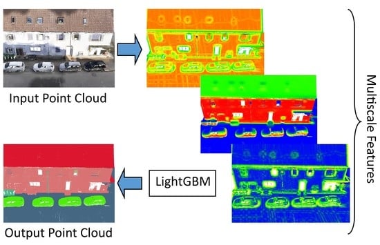
Our framework (Figure 1) follows a general framework for machine learning. The raw point cloud is subsampled to multiple levels using Poisson Sampling, and then the features are extracted for each level. LightGBM classifier is used in the classification of concatenated features of multi-level point clouds. The output has labels for each point.
We introduce each section of our framework in the following subsections. Section 3.1 defines our multiscale sampling strategy, then in Section 3.2 we show how we control the neighborhood parameters combined with our sampling method. Section 3.3 includes our feature set and Section 3.4 represents our LightGBM classifier.
3.1. Multi-Scale Sampling
Considering the various sizes of objects in the point cloud, multi-scale sampling is more inclusive than fixed sampling. In addition to that, it is not required to have all neighborhood points for the computational efficiency of feature calculation; therefore, a portion of neighborhood points is enough instead of all neighbor points.
Regular sampling, either in 2D [14] or 3D [22], is a commonly used sampling method for point clouds. However, it may cause information loss and lead to misclassification. Random sampling [40] and Furthest Point Sampling [38] are alternative methods; however, while the former requires special attention due to the random selection of points, despite its computational efficiency, the latter is computationally costly, even though its results are promising.
In this study, we select to use Poisson Disk Sampling [51] because it is more resistant to information loss according to its computational efficiency. Moreover, it only requires one parameter, the radius —the minimum distance between two points. It mainly works as a random selection of a root point and then expands the sample set considering the radius parameter. In the end, the method results in a subsampled point cloud where the distance between each point is at most the parameter of the radius.
3.2. Neighborhood Definition
Considering a multiscale framework, where at each level the neighborhood search is performed, a fast neighborhood search has to be selected for a large-scale dataset. KNN is computationally efficient, but accurately inadequate; however, RS gives more accurate results, but in a slower processing time. Besides this, parameter selection is more important in RS: a large number of neighbors may increase computation time, while a lower number of neighbors may cause the loss of useful information. While [22] uses KNN with a voxel-based structure, [14] prefers RS but with grid sampling; in other words, they convert the irregular point cloud into a regular format.
Unlike the studies above, we prefer RS with irregular subsampling points but accelerate RS with Graphical Processing Unit (GPU) support, which reduces the computational cost of RS. For a proper parameter selection, we are adopting [14]’s radius search and grid size relations as shown in Equations (1) and (2).
where refers to the radius for Poisson sampling at scale level S and is the radius for neighborhood search at scale level S, refers to the multiscale constant which controls the radius size at different multiscale levels, is a constant that determines the radius search based on Poisson sampling distance at level S. Using those formulas, we control the radii for the RS and Poisson sampling and we need to define , S and two constants of and .
3.3. Feature Extraction
While there exist various global- and local-scale features for point clouds in the literature (see [15,27]), we focus on simple and easy-to-compute features. Geometric and eigen-based features, which rely on the local neighborhood information of the points in the point cloud and give valuable information about a point’s local geometric characteristics, are commonly used feature sets in PCC studies. Let be a three-dimensional point, be a point cloud with n points and , be a local neighborhood of point p with m neighborhood points, where q are in a distance of at most r; then, the covariance matrix equals where is the average of the neighbor set of points. The eigendecomposition of the covariance matrix leads to eigenvalues (in descending order) and eigenvectors . The features of sum of eigenvalues, linearity, planarity, sphericity, omnivariance, eigenentropy, surface variation and anisotropy are easily calculated, as shown in Table 1. Absolute and vertical moments [14], as well as verticality [22], are added to the set of features to give a more distinctive set of characteristics. Although covariance features are computed from the ratios of eigenvalues and eigenvectors, height features include only information from neighborhood points without the extra cost of computation. Height information in the feature set increase the performance of the classification [18]. Accordingly, five height features are combined from statistical properties of the neighborhood. Lastly, since MLS point clouds have heterogeneous density, we add neighborhood density information to the feature set without any computational cost.
In the study, a total of 23 features per scale are defined, which consists of 17 features based on eigenvalues and of 5 height features, and a density value—a number of neighbors in the radius (Table 1). Additional features, such as intensity, echo ratio and color information, have not been considered as the main features in our experiments. However, we clearly identify additional feature sets in the experiment section of Section 4.
3.4. Classification
Decision tree ensemble learning has previously been performed for 3D PCC, based on the technique of bagging [14,22] or boosting [20]. RF [28]—a bagging-based ensemble of decision trees, which is based on a combination of tree scores from randomly created multiple decision trees—especially comes forward among them [15] and has become a popular choice of ML classifier in 3D PCC [14,21,22], and even considered as a baseline method in many benchmark datasets, such as in Kölle et al. [52] and Kharroubi et al. [53]. Gradient-boosting machines [54], however, construct a strong learner from weak learners iteratively, which is based on improving the scores according to the previous iteration. Instead of constructing the decision trees in one step, as in RF, this iterative update process makes the gradient boosting machines superior to RF in proper settings.
Let show the sample data with n instances, where defines the feature vector of dimensions m and refers to corresponding labels, gradient-boosting machine ensemble trees find the approximation of a function using K additive tree functions [31].
where is the weight of the decision tree function of . A loss function is minimized in each iteration until the maximum number of iterations or the solution converges.
Several variants of gradient boosting machines have appeared in recent years. Xgboost [29], while following the gradient boosting machine framework, adds regularization terms to the loss function to prevent overfitting. Other improvements include the implementation of random sampling and column subsampling, a faster best-split finding method and the usage of second-order derivatives in the loss function. LightGBM [30], in contrast, focuses on computational efficiency in gradient-boosting machines, particularly with big data. Therefore, it improves the best split finding with Gradient-based one-side sampling (GOSS) and Exclusive feature blending (EFB), where unimportant samples are removed and common features are merged, respectively. Considering our large-scale data and multi-scale features, we have selected LightGBM as our classifier in this study.
4. Experimental Results and Discussion
In this section, we represent our three benchmark datasets in Section 4.1; then, we introduce our implementation tools in Section 4.2. Next, we define training and testing strategies and parameters for our proposed framework on the datasets and present both numerical and visual results with discussion in Section 4.4 following the evaluation framework in Section 4.3. We perform a comparative study in Section 4.5 and, lastly, we conduct an ablation study in Section 4.6.
4.1. Datasets
Publicly available datasets make it possible to compare the performance of the proposed framework with previous studies on a common platform without any data-intensive efforts. They also provide a shareable scientific environment for the community and increase the impact of research by combining several solutions on the same dataset. In particular, there exist several LiDAR point cloud benchmark datasets in the literature, from a variety of platforms (Airborne, Terrestrial, etc.) and types (static and dynamic). However, for static MLS datasets only a few options are available.
We selected the Paris–rue–Madame dataset since it was one of the first available urban MLS benchmark datasets, while Paris–rue–Cassette provides a similar urban environment with fewer points but more classes. These two datasets differ from their ancestors based on their point size in a dense urban area with complex structures of urban objects. Another dataset, on the other hand, Toronto-3D, involves roadside urban objects and it is one of the latest available datasets for MLS data. Overall, having a diverse urban environment and semantic categories allows us to test our proposed framework in different settings. In the next subsections, we briefly describe our datasets and give a summary of the class statistics in the tables.
4.1.1. Paris-rue-Madame Database
Paris–rue–Madame [55] was acquired from the streets of Paris, France, with the LARA2-3D mobile mapping system. The dataset includes a 160 m street section with ≈20 M points. Following [15], we ignore the smaller classes and focus on six classes: facade, ground, cars, motorcycles, traffic signs and pedestrians (see Table 2).
4.1.2. Paris-rue-Cassette Database
Similarly, this mobile LiDAR dataset [56] was acquired from Paris, France, with a StereopolisII mobile mapping system. It contains ≈12 M points from a 200 m street section. Like the previous dataset, we are using only seven dominant classes: facade, ground, cars, motorcycles, traffic signs, pedestrians and vegetation.
Note that both the Paris–rue–Madame and Paris–rue–Cassette datasets share similar class characteristics, but the former includes one more class in a smaller point size. A summary of both datasets is given in Table 2.
4.1.3. Toronto-3D Mobile LiDAR Dataset
Toronto-3D mobile LiDAR dataset [57] was acquired from the Teledyne Optech Maverick mobile mapping system in Toronto, Canada. It contains a 1000 m section with a total of 76M points. It also includes eight classes: Road marker, natural, building, utility line, pole, car and fence. Data are publicly available as four tiles, and we are following the data provider’s learning strategy [57], where we pick three of them as training and one of them used as testing. A summary of the samples is given in Table 3.
4.2. Implementation
Our implementation consists of various tools: Multiscale sampling is performed using the Point Data Abstraction Library (PDAL) [58,59]. Feature extraction implementation is on a partially graphical processing unit (GPU) and multi-core central processing unit (CPU). Radius search and finding neighborhood points are implemented on GPU with Point Cloud Library [60], and feature calculation is performed on a multicore CPU in parallel, all written in C++. Python programming language is used for classification experiments with LightGBM. The experiment is all conducted in an NVIDIA RTX 4000M 8 GB graphics card and 4-cores Xeon-W2225 4.1 GHz computing power unit with 64 GB RAM.
4.3. Evaluation
We evaluate the results both qualitatively and quantitatively. We report the quantitative results in the precision (P) (Equation (4)), recall (R) (Equation (5)) and F1-measure (F1) (Equation (6)) metrics for each class in each experiment, as we also take those metrics’ average for overall evaluation. For consistency with previous studies [14,57], we report the performance of the classification results using Intersection over Union (IoU) (Equation (8)) as a class-level indicator and the average of IoU and overall precision (OA) (Equation (7)) as global indicators.
where , , and refer to true positives and negatives, false positives and negatives, respectively. The average score per metric is the ratio of the sum of the scores to the number of classes.
We show qualitative results for each experiment, whereas we pay attention to demonstrate erroneous labels, which help to understand the performance of the proposed framework. In addition, we report the feature extraction and training times for comparison with the previous studies.
4.4. Experiments and Discussion
We evaluated three urban LiDAR point clouds using the proposed methodology. We followed the same training and testing strategy as [15] for Paris-rue-Madame and Paris-rue-Cassette, while we used the provided training /testing tiles for the Toronto-3D dataset following the same strategy as [57]. Since two of the datasets share similar properties, Paris-rue-Madame and Paris-rue-Cassette, we report their experiments together in the next subsection.
4.4.1. Paris–rue–Madame and Paris–rue–Cassette Databases
We used identical parameters for the two datasets. As aforementioned in Section 3.2, we select , , and , which means we have a total of 184 + 3 (xyz) features. We use the feature set in Table 1, and do not use intensity, color or echo information for a fair comparison with previous studies. We randomly select 1000 points per class and use those as training and the rest for testing, which means that we have 6000 and 7000 training samples for Paris–rue–Cassette and Paris–rue–Madame, respectively. As shown in Table 2, selecting an equal number of training samples overcomes the class imbalance problem, where we did not need oversampling techniques. We trained selected data samples with 1000 iterations, 0.05 learning rate, 512 max bins, 0.35 feature fraction rate, 8 max depth, 90 number of leaves and a 0.50 subsample rate for both datasets in the LightGBM classifier. Multiscale parameters were estimated heuristically and a grid search was used to estimate the classifier parameters. Overall, as in Thomas et al. [14], we repeat the selection of random points for training several times and report the mean of those attempts.
After applying our framework to the two datasets, we obtain the results shown in Table 4 and Table 5. Both experiments achieved a high OA score of and for Paris–rue–Madame and Paris–rue–Cassette, respectively. Similarly, even though average recall scores are above for both experiments, we have lower precision scores, for Paris–rue–Madame and for Paris–rue–Cassette, which means that our framework tends to label samples correctly with a low false negative rate but at the same time suffers from incorrect positive labels with a high false positive rate.
On the other hand, our framework had both in precision and recall for large-sized objects—facade and grounds—and also medium-sized objects–cars—in both experiments. Since our framework takes advantage of the multiscale feature extractor, we reach metrics for those classes. Small objects, on the contrary, have better scores in the Paris–rue–Madame experiment than in the Paris–rue–Cassette experiment, where the sample size of the classes may affect the classification.
To verify the quantitative results, we take the visuals from both experiments as shown in Figure 2. According to the erroneous figure, our framework cannot distinguish the points on the boundaries; for instance, the traffic lights were able to be extracted clearly, but mistakenly ground points were also labeled as traffic lights, which is an indicator of higher recall and lower precision scores. There is a similar misclassification for the ground and facade classes, where two classes share similar geometric properties at the boundaries. The definition of the neighborhood may be the reason behind this misclassification; at the boundaries, it is unavoidable to have information from the neighbors; therefore, misclassification occurring at the boundaries is one of the drawbacks of the framework.
4.4.2. Toronto-3D
Following similar principles in two previous experiments, we select , , and for the parts of the definition of neighborhood and the extraction of features in this experiment. In addition to the feature set in Table 1, we used color (converted to HSV space) and intensity with their averages and variances, which led to a feature size of 210 + 3 (xyz). We follow the training/testing splits [57] and use the L002 area as the testing site. In training, we are selecting 350 K points from each class, considering the equal number of samples from each class and the lowest sampled class. Thus, we had a 2.8 M points training sample and used our LightGBM classifier based on these samples. However, like our previous samples, we randomly selected training samples a few times and reported their averages. We found the optimal parameters through a grid search for our classifier: 0.03 learning rate, 607 max bins, 0.66 feature fraction rate, 10 max depth, 210 number of leaves, and 0.70 subsample rate for the datasets. We trained our ensemble in 250 iterations.
Next, we applied our framework to the Toronto3D dataset and received the following numerical metrics, shown in Table 6. We reach OA, average precision and average recall scores. Similarly to the two previous experiments, our framework obtains high-recall and low-precision scores. We reach for almost all classes in precision and recall scores, except for the road marking and fence classes. Although we reached on the recall score on the road markings, only were correctly labeled. The fence class has the worst scores of all the evaluation metrics in the experiment.
To illustrate, we created a top-view image from a part of the dataset (Figure 3) as well as detailed visuals (Figure 4) for this experiment. We can infer from the top-view image that our framework mislabels the class boundaries. Moreover, when the size of object is small, then a part of the object is misclassified.
Road marking and road classes are one of the best examples of the boundary effect in our framework. As shown in Figure 4 in the top row, the class of road and road markings has a large confusion; therefore, we obtain incorrect labels in the last column of the figure. The reason behind this is to accumulate local information through the radius neighborhood. When the object size is small, like an object of fence class in Figure 4 at the bottom row, our framework partly mislabels the object.
Descriptive features also play a key role in misclassification, as distinguishing road marking classes from roads requires RGB or intensity information; otherwise, these two classes have common geometric structures. The same problem arises in a pole in the bottom row of Figure 4, which was mistakenly labeled building. Similar misclassification errors exist in pole and utility lines, as well as in ground and car classes.
In addition to numerical and visual results, we also report feature calculation and training time because these operations are one of the keys to large-scale datasets. Our feature extraction module outputs the Paris–rue–Cassette in 255 s, including reading and writing the files. When we compare with previous studies, we can infer that our implementation of feature extraction is on par with Thomas et al. [14], Hackel et al. [22], which had 319 and 191 s in the same settings of the same experiment. We all took advantage of parallel processing, but Thomas et al. [14] and Hackel et al. [22] used a hierarchical data structure that made processing faster. Our implementation’s radius search was on the GPU despite having irregular subsampled point clouds. It should be noted that the processing time for feature calculation depends on the implementation details and the computer hardware. The training in Paris–rue–Madame, however, took approximately 10 s in our settings, where the RF training time was 3 s in the same experiment. One of the factors for training time is the number of samples: having a large sample size increases the training time. In Paris–rue–Cassette, the training time was 14 s on average, and the training took 13 min on average in the Toronto-3D experiment.
4.5. Comparison with the Previous Studies
We use our three dataset results in a two-fold comparison with previous studies: (i) We compare our results with previous studies focusing on an RF classifier. For this purpose, we only use the Paris–rue–Madame and Paris–rue–Cassette experiments. (ii) We focus on DL methods in the Toronto-3D experiment. As mentioned above in Section 4.3, we are evaluating our frameworks using IoU per class, and the mean IoU (mIoU) and OA for overall scores.
In the first, we compare our results for the Paris–rue–Madame and Paris–rue–Cassette datasets, as the scores were given in Table 7 with the results of previous studies. Considering that previous studies [14,22] were used to classify RF and their set of characteristics was similar to ours, we can infer that our LightGBM improves the results compared to RF. Although the RF is giving worse accuracy results, it is faster than LightGBM in training. More clearly, for a 7000 sample training set in the Paris–rue–Madame dataset, the RF took 3 s, while LightGBM trained the same samples in 9 s. In addition, LightGBM requires more parameters to tune in training. Consequently, it is clear that there is a trade-off between computational complexity and accuracy performance in the ensemble learning of decision trees. According to the results, we have the highest scores for almost all classes, only the pedestrian class score is second place. Furthermore, our mean IoU scores improve the best study to 2.48% and 10.01% for the Paris–rue–Madame and Paris–rue–Cassette datasets, respectively. An important improvement in the rue Madame dataset is the motorcycles class, while in the rue Cassette almost all classes, except ground and facade, are importantly improved.
In the second, we compare the Toronto-3D results with DL-based models, as shown in Table 8. It is clear that, even though our framework did not supersede the DL-based methods, it is on par with most of the methods. It is worth noting that the results in Table 8 show the xyz processing results, where * and ** refer to the use of additional features, RGB and intensity, respectively. This is the reason why these models have the worst scores in the road marking class, which requires additional features such as color or intensity. For a fair comparison, we consider only Hu et al. [40], Yan et al. [61], Rim et al. [62] and Han et al. [63]. Among the various methods mentioned, our framework has the best overall accuracy score. However, [57] has the best scores despite using only xyz values. Our mIoU scores, in contrast, are on the same page with others, while [40,61] passed the 80% threshold. For class level results, the classes of road, natural, building, car and utility line have the IoU scores on the page with others. It is evident that [40,61] dominates the results in all classes.
The main reason behind having the results on the same page with deep learning models is that our feature set does not only include geometric features but also other discriminative features, which are RGBs, intensity and height features. It should be noted that our height feature set consists of basic statistical values and does not depend on additional data sources, such as height from a digital surface model.
4.6. Ablation Study
We perform our ablation study on the Toronto-3D dataset. We observe the impact of training point selection, sampling methods, and the number of multiscale levels.
4.6.1. Impact of Training Point Selection
In training, we select a constant number of points to avoid class imbalance of the data. Some classes have dominant classes, while others have minimum samples. Therefore, the selection of training points is the first effect of the training procedure. We select training samples a few times, reproduce the results of those samples, and plot their distribution as the boxplot shown in Figure 5. We only consider OA and mIoU scores. For both scores, we did not observe any outliers, and the range between minimum and maximum was ≈0.35% and ≈0.40%, for OA and mIoU, respectively.
4.6.2. Sampling Methods
We compare our framework sampling method with random and voxel-based sampling methods. We reduce the number of points by half at each level in random sampling and use voxel sizes identical to Poisson sampling in voxel-based sampling. Keeping the radius of the neighborhood search the same at each level and taking the highest score samples, we achieved the following results shown in Table 9.
According to the results from different samplings, we are reaching the highest score from Poisson sampling, while random sampling gives the worst results. Poisson sampling increases the mean IoU by and compared to random sampling and voxel-based sampling, respectively. It is interesting that for both Poisson sampling and random sampling, OA scores are almost identical.
4.6.3. Multi-Scale Levels
We use a few multiscale levels in the classification. As shown in Figure 6, after scale 6, our scores start to decrease; therefore, we use six scales in the classification. It shows that our model cannot increase the model accuracy after having additional multiscale features of scale 7. Adding more samples should improve the model’s accuracy.
5. Conclusions
In this study, we proposed a general ML framework for 3D PCC using the LightGBM classifier. Our framework took advantage of multiscale feature extraction and classifier performance; thus, it had better results compared to traditional RF classifiers, while giving promising results against state-of-the-art deep learning models. However, it is worth noting that our training procedure requires fewer samples than DL models; therefore, our model is more energy-efficient. Also, we use simple geometric features and height features. It is known that, with more distinctive results, the accuracy of the results increases. With an improved feature set, such as height from digital terrain models or additional neighborhood types, the results have the potential to improve, but computation cost should be considered for training in LightGBM. Moreover, we used only LightGBM; instead, evaluation of other GBMs and ML methods in PCC is required for further research. Lastly, we are planning to test our framework with other available benchmark datasets.
Author Contributions
Conceptualization, E.S. and S.A.; methodology, E.S.; software, E.S.; validation, E.S.; formal analysis, E.S.; investigation, E.S.; resources, E.S.; data processing, E.S.; writing—original draft preparation, E.S.; writing—review and editing, S.A.; visualization, E.S.; supervision, S.A. All authors have read and agreed to the published version of the manuscript.
Funding
This research received no external funding.
Institutional Review Board Statement
Not applicable.
Informed Consent Statement
Not applicable.
Data Availability Statement
Not applicable.
Acknowledgments
This study is part of the first author’s Ph.D. thesis. We thank the dataset providers. Paris–rue–Madame dataset is available at https://people.cmm.minesparis.psl.eu/users/serna/rueMadameDataset.html. MINES ParisTech created this special set of 3D MLS data for the purpose of detection–segmentation–classification research activities, but does not endorse the way they are used in this project or the conclusions put forward. The Paris–rue–Cassette database is publicly available at http://data.ign.fr/benchmarks/UrbanAnalysis/. We reached the Toronto-3D dataset through https://github.com/WeikaiTan/Toronto-3D. All datasets were accessed on 18 April 2023.
Conflicts of Interest
The authors declare no conflict of interest.
References
- Puente, I.; González-Jorge, H.; Martínez-Sánchez, J.; Arias, P. Review of mobile mapping and surveying technologies. Measurement 2013, 46, 2127–2145. [Google Scholar] [CrossRef]
- Li, Y.; Ma, L.; Zhong, Z.; Liu, F.; Chapman, M.A.; Cao, D.; Li, J. Deep Learning for LiDAR Point Clouds in Autonomous Driving: A Review. IEEE Trans. Neural Netw. Learn. Syst. 2021, 32, 3412–3432. [Google Scholar] [CrossRef] [PubMed]
- Wang, R.; Peethambaran, J.; Chen, D. LiDAR Point Clouds to 3-D Urban Models: A Review. IEEE J. Sel. Top. Appl. Earth Obs. Remote Sens. 2018, 11, 606–627. [Google Scholar] [CrossRef]
- Wang, C.; Wen, C.; Dai, Y.; Yu, S.; Liu, M. Urban 3D modeling with mobile laser scanning: A review. Virtual Real. Intell. Hardw. 2020, 2, 175–212. [Google Scholar] [CrossRef]
- Li, F.; Oude Elberink, S.; Vosselman, G. Semantic labelling of road furniture in mobile laser scanning data. Int. Arch. Photogramm. Remote Sens. Spat. Inf. Sci. 2017, 42, 247–254. [Google Scholar] [CrossRef] [Green Version]
- Chen, Y.; Wang, S.; Li, J.; Ma, L.; Wu, R.; Luo, Z.; Wang, C. Rapid Urban Roadside Tree Inventory Using a Mobile Laser Scanning System. IEEE J. Sel. Top. Appl. Earth Obs. Remote Sens. 2019, 12, 3690–3700. [Google Scholar] [CrossRef]
- Huang, J.; You, S. Pole-like object detection and classification from urban point clouds. In Proceedings of the 2015 IEEE International Conference on Robotics and Automation (ICRA), Seattle, WA, USA, 26–30 May 2015; pp. 3032–3038. [Google Scholar] [CrossRef]
- Guan, H.; Yan, W.; Yu, Y.; Zhong, L.; Li, D. Robust Traffic-Sign Detection and Classification Using Mobile LiDAR Data With Digital Images. IEEE J. Sel. Top. Appl. Earth Obs. Remote Sens. 2018, 11, 1715–1724. [Google Scholar] [CrossRef]
- Bao, Z.; Hossain, S.; Lang, H.; Lin, X. A review of high-definition map creation methods for autonomous driving. Eng. Appl. Artif. Intell. 2023, 122, 106125. [Google Scholar] [CrossRef]
- Qin, R.; Tian, J.; Reinartz, P. 3D change detection—Approaches and applications. ISPRS J. Photogramm. Remote Sens. 2016, 122, 41–56. [Google Scholar] [CrossRef] [Green Version]
- Voelsen, M.; Schachtschneider, J.; Brenner, C. Classification and Change Detection in Mobile Mapping LiDAR Point Clouds. PFG—J. Photogramm. Remote Sens. Geoinf. Sci. 2021, 89, 195–207. [Google Scholar] [CrossRef]
- Xie, Y.; Tian, J.; Zhu, X.X. Linking Points With Labels in 3D: A Review of Point Cloud Semantic Segmentation. IEEE Geosci. Remote Sens. Mag. 2020, 8, 38–59. [Google Scholar] [CrossRef] [Green Version]
- Guo, Y.; Wang, H.; Hu, Q.; Liu, H.; Liu, L.; Bennamoun, M. Deep Learning for 3D Point Clouds: A Survey. IEEE Trans. Pattern Anal. Mach. Intell. 2021, 43, 4338–4364. [Google Scholar] [CrossRef] [PubMed]
- Thomas, H.; Goulette, F.; Deschaud, J.E.; Marcotegui, B.; LeGall, Y. Semantic Classification of 3D Point Clouds with Multiscale Spherical Neighborhoods. In Proceedings of the 2018 International Conference on 3D Vision (3DV), Verona, Italy, 5–8 September 2018; pp. 390–398. [Google Scholar] [CrossRef] [Green Version]
- Weinmann, M.; Jutzi, B.; Hinz, S.; Mallet, C. Semantic point cloud interpretation based on optimal neighborhoods, relevant features and efficient classifiers. ISPRS J. Photogramm. Remote Sens. 2015, 105, 286–304. [Google Scholar] [CrossRef]
- Brodu, N.; Lague, D. 3D terrestrial lidar data classification of complex natural scenes using a multi-scale dimensionality criterion: Applications in geomorphology. ISPRS J. Photogramm. Remote Sens. 2012, 68, 121–134. [Google Scholar] [CrossRef] [Green Version]
- Wang, L.; Huang, Y.; Hou, Y.; Zhang, S.; Shan, J. Graph attention convolution for point cloud semantic segmentation. In Proceedings of the IEEE/CVF Conference on Computer Vision and Pattern Recognition, Long Beach, CA, USA, 15–20 June 2019; pp. 10296–10305. [Google Scholar]
- Niemeyer, J.; Rottensteiner, F.; Soergel, U. Contextual classification of lidar data and building object detection in urban areas. ISPRS J. Photogramm. Remote Sens. 2014, 87, 152–165. [Google Scholar] [CrossRef]
- Blomley, R.; Jutzi, B.; Weinmann, M. Classification of airborne laser scanning data using geometric multi-scale features and different neighbourhood types. ISPRS Ann. Photogramm. Remote Sens. Spat. Inf. Sci. 2016, 3, 169–176. [Google Scholar] [CrossRef] [Green Version]
- Guo, B.; Huang, X.; Zhang, F.; Sohn, G. Classification of airborne laser scanning data using JointBoost. ISPRS J. Photogramm. Remote Sens. 2015, 100, 71–83. [Google Scholar] [CrossRef]
- Weinmann, M.; Schmidt, A.; Mallet, C.; Hinz, S.; Rottensteiner, F.; Jutzi, B. Contextual classification of point cloud data by exploiting individual 3D neigbourhoods. ISPRS Ann. Photogramm. Remote Sens. Spat. Inf. Sci. 2015, 2, 271–278. [Google Scholar] [CrossRef] [Green Version]
- Hackel, T.; Wegner, J.D.; Schindler, K. Fast Semantic Segmentation of 3D Point Clouds with Strongly Varying Density. ISPRS Ann. Photogramm. Remote Sens. Spat. Inf. Sci. 2016, 3, 177–184. [Google Scholar] [CrossRef] [Green Version]
- Demantké, J.; Mallet, C.; David, N.; Vallet, B. Dimensionality based scale selection in 3D lidar point clouds. Int. Arch. Photogramm. Remote Sens. Spat. Inf. Sci. 2012, 38, 97–102. [Google Scholar] [CrossRef] [Green Version]
- Blomley, R.; Weinmann, M. Using multi-scale features for the 3D semantic labeling of airborne laser scanning data. ISPRS Ann. Photogramm. Remote Sens. Spat. Inf. Sci. 2017, 4, 43–50. [Google Scholar] [CrossRef] [Green Version]
- Chehata, N.; Guo, L.; Mallet, C. Airborne lidar feature selection for urban classification using random forests. In Proceedings of the ISPRS Workshop Laserscanning’09, Paris, France, 1–2 September 2009; pp. 207–212. [Google Scholar]
- Weinmann, M.; Urban, S.; Hinz, S.; Jutzi, B.; Mallet, C. Distinctive 2D and 3D features for automated large-scale scene analysis in urban areas. Comput. Graph. 2015, 49, 47–57. [Google Scholar] [CrossRef]
- Han, X.F.; Sun, S.J.; Song, X.Y.; Xiao, G.Q. 3D Point Cloud Descriptors in Hand-crafted and Deep Learning Age: State-of-the-Art. arXiv 2020, arXiv:1802.02297. [Google Scholar]
- Breiman, L. Random Forests. Mach. Learn. 2001, 45, 5–32. [Google Scholar] [CrossRef] [Green Version]
- Chen, T.; Guestrin, C. XGBoost: A Scalable Tree Boosting System. In Proceedings of the 22nd ACM SIGKDD International Conference on Knowledge Discovery and Data Mining, KDD ’16, San Francisco, CA, USA, 13–17 August 2016; ACM: New York, NY, USA, 2016; pp. 785–794. [Google Scholar] [CrossRef] [Green Version]
- Ke, G.; Meng, Q.; Finley, T.; Wang, T.; Chen, W.; Ma, W.; Ye, Q.; Liu, T.Y. Lightgbm: A highly efficient gradient boosting decision tree. Adv. Neural Inf. Process. Syst. 2017, 30, 3146–3154. [Google Scholar]
- Bentéjac, C.; Csörgő, A.; Martínez-Muñoz, G. A comparative analysis of gradient boosting algorithms. Artif. Intell. Rev. 2021, 54, 1937–1967. [Google Scholar] [CrossRef]
- Su, H.; Maji, S.; Kalogerakis, E.; Learned-Miller, E. Multi-view convolutional neural networks for 3d shape recognition. In Proceedings of the IEEE International Conference on Computer Vision, Santiago, Chile, 7–13 December 2015; pp. 945–953. [Google Scholar]
- Tatarchenko, M.; Park, J.; Koltun, V.; Zhou, Q.Y. Tangent convolutions for dense prediction in 3d. In Proceedings of the IEEE Conference on Computer Vision and Pattern Recognition, Salt Lake City, UT, USA, 18–23 June 2018; pp. 3887–3896. [Google Scholar]
- Boulch, A.; Le Saux, B.; Audebert, N. Unstructured point cloud semantic labeling using deep segmentation networks. 3dor@ Eurographics 2017, 3, 17–24. [Google Scholar]
- Riegler, G.; Osman Ulusoy, A.; Geiger, A. Octnet: Learning deep 3d representations at high resolutions. In Proceedings of the IEEE Conference on Computer Vision and Pattern Recognition, Honolulu, HI, USA, 21–26 July 2017; pp. 3577–3586. [Google Scholar]
- Maturana, D.; Scherer, S. Voxnet: A 3d convolutional neural network for real-time object recognition. In Proceedings of the 2015 IEEE/RSJ International Conference on Intelligent Robots and Systems (IROS), Hamburg, Germany, 28 September–2 October 2015; pp. 922–928. [Google Scholar]
- Wang, L.; Huang, Y.; Shan, J.; He, L. MSNet: Multi-Scale Convolutional Network for Point Cloud Classification. Remote Sens. 2018, 10, 612. [Google Scholar] [CrossRef] [Green Version]
- Qi, C.R.; Su, H.; Mo, K.; Guibas, L.J. Pointnet: Deep learning on point sets for 3d classification and segmentation. In Proceedings of the IEEE Conference on Computer Vision and Pattern Recognition, Honolulu, HI, USA, 21–26 July 2017; pp. 652–660. [Google Scholar]
- Qi, C.R.; Yi, L.; Su, H.; Guibas, L.J. Pointnet++: Deep hierarchical feature learning on point sets in a metric space. In Proceedings of the Advances in Neural Information Processing Systems, Long Beach, CA, USA, 4–9 December 2017; Volume 30. [Google Scholar]
- Hu, Q.; Yang, B.; Xie, L.; Rosa, S.; Guo, Y.; Wang, Z.; Trigoni, N.; Markham, A. Randla-net: Efficient semantic segmentation of large-scale point clouds. In Proceedings of the IEEE/CVF Conference on Computer Vision and Pattern Recognition, Seattle, WA, USA, 13–19 June 2020; pp. 11108–11117. [Google Scholar]
- Zhao, H.; Jiang, L.; Fu, C.W.; Jia, J. Pointweb: Enhancing local neighborhood features for point cloud processing. In Proceedings of the IEEE/CVF Conference on Computer Vision and Pattern Recognition, Long Beach, CA, USA, 15–20 June 2019; pp. 5565–5573. [Google Scholar]
- Li, Y.; Bu, R.; Sun, M.; Wu, W.; Di, X.; Chen, B. Pointcnn: Convolution on x-transformed points. In Proceedings of the Advances in Neural Information Processing Systems, Montreal, QC, Canada, 3–8 December 2018; Volume 31. [Google Scholar]
- Wu, W.; Qi, Z.; Fuxin, L. Pointconv: Deep convolutional networks on 3d point clouds. In Proceedings of the IEEE/CVF Conference on Computer Vision and Pattern Recognition, Long Beach, CA, USA, 15–20 June 2019; pp. 9621–9630. [Google Scholar]
- Thomas, H.; Qi, C.R.; Deschaud, J.E.; Marcotegui, B.; Goulette, F.; Guibas, L.J. Kpconv: Flexible and deformable convolution for point clouds. In Proceedings of the IEEE/CVF International Conference on Computer Vision, Seoul, Republic of Korea, 27 October–2 November 2019; pp. 6411–6420. [Google Scholar]
- Xu, M.; Ding, R.; Zhao, H.; Qi, X. Paconv: Position adaptive convolution with dynamic kernel assembling on point clouds. In Proceedings of the IEEE/CVF Conference on Computer Vision and Pattern Recognition, Nashville, TN, USA, 20–25 June 2021; pp. 3173–3182. [Google Scholar]
- Wang, Y.; Sun, Y.; Liu, Z.; Sarma, S.E.; Bronstein, M.M.; Solomon, J.M. Dynamic graph cnn for learning on point clouds. ACM Trans. Graph. (Tog) 2019, 38, 1–12. [Google Scholar] [CrossRef] [Green Version]
- Engel, N.; Belagiannis, V.; Dietmayer, K. Point transformer. IEEE Access 2021, 9, 134826–134840. [Google Scholar] [CrossRef]
- Guo, M.H.; Cai, J.X.; Liu, Z.N.; Mu, T.J.; Martin, R.R.; Hu, S.M. Pct: Point cloud transformer. Comput. Vis. Media 2021, 7, 187–199. [Google Scholar] [CrossRef]
- Zhao, H.; Jiang, L.; Jia, J.; Torr, P.H.; Koltun, V. Point transformer. In Proceedings of the IEEE/CVF International Conference on Computer Vision, Montreal, BC, Canada, 10–17 October 2021; pp. 16239–16248. [Google Scholar]
- Zhang, J.; Zhao, X.; Chen, Z.; Lu, Z. A Review of Deep Learning-Based Semantic Segmentation for Point Cloud. IEEE Access 2019, 7, 179118–179133. [Google Scholar] [CrossRef]
- Cook, R.L. Stochastic Sampling in Computer Graphics. Acm Trans. Graph. 1986, 5, 51–72. [Google Scholar] [CrossRef]
- Kölle, M.; Laupheimer, D.; Schmohl, S.; Haala, N.; Rottensteiner, F.; Wegner, J.D.; Ledoux, H. The Hessigheim 3D (H3D) benchmark on semantic segmentation of high-resolution 3D point clouds and textured meshes from UAV LiDAR and Multi-View-Stereo. ISPRS Open J. Photogramm. Remote Sens. 2021, 1, 100001. [Google Scholar] [CrossRef]
- Kharroubi, A.; Van Wersch, L.; Billen, R.; Poux, F. Tesserae3d: A Benchmark for Tesserae Semantic Segmentation in 3D Point Clouds. In SPRS Annals of the Photogrammetry, Remote Sensing and Spatial Information Sciences; Copernicus: Goettingen, Germany, 2021; Volume V-2-2021, pp. 121–128. [Google Scholar] [CrossRef]
- Friedman, J.H. Greedy function approximation: A gradient boosting machine. Ann. Stat. 2001, 29, 1189–1232. [Google Scholar] [CrossRef]
- Serna, A.; Marcotegui, B.; Goulette, F.; Deschaud, J.E. Paris-rue-Madame database: A 3D mobile laser scanner dataset for benchmarking urban detection, segmentation and classification methods. In Proceedings of the 4th International Conference on Pattern Recognition, Applications and Methods ICPRAM 2014, Angers, France, 6–8 March 2014. [Google Scholar]
- Vallet, B.; Brédif, M.; Serna, A.; Marcotegui, B.; Paparoditis, N. TerraMobilita-iQmulus urban point cloud analysis benchmark. Comput. Graph. 2015, 49, 126–133. [Google Scholar] [CrossRef] [Green Version]
- Tan, W.; Qin, N.; Ma, L.; Li, Y.; Du, J.; Cai, G.; Yang, K.; Li, J. Toronto-3D: A Large-Scale Mobile LiDAR Dataset for Semantic Segmentation of Urban Roadways. In Proceedings of the IEEE/CVF Conference on Computer Vision and Pattern Recognition (CVPR) Workshops, Seattle, WA, USA, 14–19 June 2020. [Google Scholar]
- PDAL Contributors. PDAL: The Point Data Abstraction Library. 2022. Available online: https://doi.org/10.5281/zenodo.2616780 (accessed on 24 July 2023).
- Butler, H.; Chambers, B.; Hartzell, P.; Glennie, C. PDAL: An open source library for the processing and analysis of point clouds. Comput. Geosci. 2021, 148, 104680. [Google Scholar] [CrossRef]
- Rusu, R.B.; Cousins, S. 3D is here: Point Cloud Library (PCL). In Proceedings of the IEEE International Conference on Robotics and Automation (ICRA), Shanghai, China, 9–13 May 2011. [Google Scholar]
- Yan, K.; Hu, Q.; Wang, H.; Huang, X.; Li, L.; Ji, S. Continuous Mapping Convolution for Large-Scale Point Clouds Semantic Segmentation. IEEE Geosci. Remote Sens. Lett. 2022, 19, 1–5. [Google Scholar] [CrossRef]
- Rim, B.; Lee, A.; Hong, M. Semantic Segmentation of Large-Scale Outdoor Point Clouds by Encoder–Decoder Shared MLPs with Multiple Losses. Remote Sens. 2021, 13, 3121. [Google Scholar] [CrossRef]
- Han, X.; Dong, Z.; Yang, B. A point-based deep learning network for semantic segmentation of MLS point clouds. ISPRS J. Photogramm. Remote Sens. 2021, 175, 199–214. [Google Scholar] [CrossRef]
- Ma, L.; Li, Y.; Li, J.; Tan, W.; Yu, Y.; Chapman, M.A. Multi-Scale Point-Wise Convolutional Neural Networks for 3D Object Segmentation From LiDAR Point Clouds in Large-Scale Environments. IEEE Trans. Intell. Transp. Syst. 2021, 22, 821–836. [Google Scholar] [CrossRef]
- Li, Y.; Ma, L.; Zhong, Z.; Cao, D.; Li, J. TGNet: Geometric Graph CNN on 3-D Point Cloud Segmentation. IEEE Trans. Geosci. Remote Sens. 2020, 58, 3588–3600. [Google Scholar] [CrossRef]
Figure 1.
The proposed framework. PC, SPC and FM refer to point cloud, subpoint cloud and feature matrix, respectively. Each color in FM represents a column-wise feature while each color in the output PC shows a semantic class.
Figure 1.
The proposed framework. PC, SPC and FM refer to point cloud, subpoint cloud and feature matrix, respectively. Each color in FM represents a column-wise feature while each color in the output PC shows a semantic class.

Figure 2.
Visual comparisons for the Paris–rue–Madame (top-row) and Paris–rue–Cassette (bottom-row) datasets. Ground truth, predicted and erroneous labels are ordered in the left, middle and right columns, respectively. Class labels are color encoded at the bottom of the figure, which is best viewed in color.

Figure 3.
A top view for visual comparison of Toronto-3D dataset’s results. Ground truth (left), predicted (middle) and erroneous (right) labels are encoded according to the color scale at the bottom. Best viewed in color.
Figure 3.
A top view for visual comparison of Toronto-3D dataset’s results. Ground truth (left), predicted (middle) and erroneous (right) labels are encoded according to the color scale at the bottom. Best viewed in color.

Figure 4.
The detailed visuals for the Toronto-3D dataset’s results. Ground truth (left), predicted (middle) and erroneous (right) labels encoded according to the color scale at the bottom. The white rectangle shows the confusion between road and road marking classes at the top row, fence, building and pole classes at the bottom row. Best viewed in color.

Figure 5.
Box plot of Toronto-3D experiment. Sampled from eleven experiments. The orange lines and the green triangles show median and mean, respectively.
Figure 5.
Box plot of Toronto-3D experiment. Sampled from eleven experiments. The orange lines and the green triangles show median and mean, respectively.

Figure 6.
Multi-scale effect in the classification. OA (above) and mIOU (below) scores are shown.


Table 1.
Summary of feature set in the study.
| Feature | Description |
|---|---|
| Sum of eigenvalues | |
| Linearity | |
| Planarity | |
| Sphericity | |
| Omnivariance | |
| Eigenentropy | |
| Surface variation | |
| Anisotropy | |
| Absolute Moment (6) | |
| Vertical moment (2) | |
| Verticality | |
| Height range | |
| Height above min | |
| Height below max | |
| Average height | |
| Height variance | |
| Density |
Table 2.
Number of samples per class (thousand) in Paris–rue–Madame and Paris–rue–Cassette experiments.
Table 2.
Number of samples per class (thousand) in Paris–rue–Madame and Paris–rue–Cassette experiments.
| Datasets | Classes | Total | ||||||
|---|---|---|---|---|---|---|---|---|
| Facade | Ground | Cars | Mtrcl | T.Signs | Pedest. | Veg. | ||
| Paris–rue–Madame | 9978.43 | 8024.30 | 1835.38 | 10.05 | 98.87 | 15.48 | - | 19,962.51 |
| Paris–rue–Cassette | 7027.02 | 4229.64 | 368.27 | 40.33 | 46.1 | 24.0 | 212.13 | 11,947.49 |
Table 3.
Number of samples per class (thousand) for training and testing tiles in Toronto-3D experiment.
Table 3.
Number of samples per class (thousand) for training and testing tiles in Toronto-3D experiment.
| Datasets | Classes | Total | |||||||
|---|---|---|---|---|---|---|---|---|---|
| Road | Road Mrk. | Natural | Building | U.Line | Pole | Car | Fence | ||
| Training | 35,391.89 | 1449.31 | 4650.92 | 18,252.78 | 589.86 | 743.58 | 4311.63 | 356.46 | 65,746.43 |
| Testing | 6305.46 | 296.14 | 1921.65 | 883.71 | 85.04 | 154.25 | 323.00 | 18.26 | 9987.52 |
Table 4.
Per class scores for Paris–rue–Madame database. The precision, recall and F1-measure is the average of eleven experiments.
Table 4.
Per class scores for Paris–rue–Madame database. The precision, recall and F1-measure is the average of eleven experiments.
| Class Name | Precision | Recall | F1-Measure |
|---|---|---|---|
| Facade | 99.10 | 99.36 | 99.23 |
| Ground | 99.38 | 97.99 | 98.68 |
| Cars | 97.61 | 99.41 | 98.50 |
| Pedest. | 80.27 | 99.91 | 88.94 |
| Mtrcl. | 69.22 | 99.13 | 81.49 |
| T.Signs | 70.19 | 99.39 | 82.19 |
| Average | 85.96 | 99.20 | 91.50 |
Table 5.
Per class scores for Paris-Rue-Cassette database. The precision, recall and F1-measure are the average of eleven experiments.
Table 5.
Per class scores for Paris-Rue-Cassette database. The precision, recall and F1-measure are the average of eleven experiments.
| Class Name | Precision | Recall | F1-Measure |
|---|---|---|---|
| Facade | 99.91 | 97.94 | 98.61 |
| Ground | 99.51 | 99.05 | 99.28 |
| Cars | 92.64 | 98.88 | 95.65 |
| Mtrcl. | 68.51 | 99.47 | 81.07 |
| T.Signs | 43.83 | 97.92 | 60.49 |
| Pedest. | 42.49 | 99.06 | 59.36 |
| Veg. | 87.37 | 98.85 | 92.74 |
| Average | 76.32 | 98.74 | 83.93 |
Table 6.
Per class scores for Toronto-3D. The precision, recall and F1-measure are the average of eleven experiments.
Table 6.
Per class scores for Toronto-3D. The precision, recall and F1-measure are the average of eleven experiments.
| Class Name | Precision | Recall | F1-Measure |
|---|---|---|---|
| Road | 99.43 | 95.03 | 97.18 |
| Road Mrk. | 50.09 | 93.27 | 65.17 |
| Natural | 97.71 | 97.07 | 97.39 |
| Buildings | 95.03 | 93.93 | 94.48 |
| Util. Line | 83.70 | 90.48 | 86.95 |
| Pole | 82.27 | 87.53 | 84.82 |
| Cars | 91.54 | 97.79 | 94.57 |
| Fence | 32.10 | 45.75 | 37.72 |
| Average | 78.98 | 87.61 | 82.29 |
Table 7.
Comparison with the previous studies for both Paris–rue–Madame (the first on each row) and Paris–rue–Cassette (the second on each row) dataset. The class scores are IoU metrics, which were obtained from Thomas et al. [14], whereas the global OA score was obtained from the studies of Hackel et al. [22] and Weinmann et al. [15]. Bold font indicates the best on the column.
| Study | Facade | Ground | Cars | Mtrcl. | T.Signs | Pedest. | Veg. | mIoU | OA |
|---|---|---|---|---|---|---|---|---|---|
| [14] | 98.22 | 96.62 | 95.37 | 61.55 | 67.43 | 77.86 | - | 82.84 | - |
| 97.27 | 97.77 | 84.94 | 58.99 | 12.71 | 35.31 | 71.48 | 65.50 | - | |
| [22] | 97.06 | 96.29 | 89.09 | 47.44 | 33.96 | 24.13 | - | 58.89 | 97.55 |
| 93.89 | 96.99 | 80.88 | 51.33 | 18.58 | 24.69 | 51.40 | 54.08 | 95.43 | |
| [15] | 91.81 | 84.88 | 55.48 | 9.44 | 4.90 | 1.63 | - | 31.68 | 88.62 |
| 86.65 | 95.75 | 47.31 | 17.12 | 14.29 | 9.06 | 24.63 | 35.30 | 89.60 | |
| Ours | 98.47 | 97.39 | 97.04 | 68.80 | 69.89 | 80.22 | - | 85.30 | 98.91 |
| 97.86 | 98.57 | 91.68 | 68.26 | 43.42 | 42.32 | 86.49 | 75.51 | 98.39 |
Table 8.
Results of Toronto-3D experiment. The best values are taken from the benchmark website. The bold indicates the first places in the column.
Table 8.
Results of Toronto-3D experiment. The best values are taken from the benchmark website. The bold indicates the first places in the column.
| Method | Road | Road Mrk. | Natural | Bldg | Util. Line | Pole | Car | Fence | mIoU | OA |
|---|---|---|---|---|---|---|---|---|---|---|
| PointNet++ SSG [39] | 89.27 | 0.00 | 69.0 | 54.1 | 43.7 | 23.3 | 52.0 | 3.0 | 41.81 | 84.88 |
| PointNet++ MSG [39] | 92.90 | 0.00 | 86.13 | 82.15 | 60.96 | 62.81 | 76.41 | 14.43 | 59.47 | 92.56 |
| DGCNN [46] | 93.88 | 0.00 | 91.25 | 80.39 | 62.40 | 62.32 | 88.26 | 15.81 | 61.79 | 94.24 |
| KPConv [44] | 94.62 | 0.06 | 96.07 | 91.51 | 87.68 | 81.56 | 85.66 | 15.72 | 69.11 | 95.39 |
| MS-PCNN [64] | 93.84 | 3.83 | 93.46 | 82.59 | 67.80 | 71.95 | 91.12 | 22.50 | 65.89 | 90.03 |
| TG-Net [65] | 93.54 | 0.00 | 90.83 | 81.57 | 65.26 | 62.98 | 88.73 | 7.85 | 61.34 | 94.08 |
| MS-TG-Net [57] | 94.41 | 17.19 | 95.72 | 88.83 | 76.01 | 73.97 | 94.24 | 23.64 | 70.50 | 95.71 |
| RandlaNet * [40] | 96.69 | 64.21 | 96.92 | 94.24 | 88.06 | 77.84 | 93.37 | 42.86 | 81.77 | 94.37 |
| MapConvSeg * [61] | 97.15 | 67.87 | 97.55 | 93.75 | 86.88 | 82.12 | 93.72 | 44.11 | 82.89 | 94.72 |
| [62] * | 92.84 | 27.43 | 89.90 | 95.27 | 85.59 | 74.50 | 44.41 | 58.30 | 71.03 | 83.60 |
| [63] ** | 92.20 | 53.80 | 92.80 | 86.00 | 72.20 | 72.50 | 75.70 | 21.20 | 70.80 | 93.60 |
| Ours | 94.52 | 48.34 | 94.91 | 89.54 | 75.92 | 73.64 | 89.69 | 23.24 | 73.85 | 95.12 |
Additional * RGB and ** Intensity with normal features were used.
Table 9.
Different sampling methodologies affect the results.
| Metric | Poisson | Random | Voxel |
|---|---|---|---|
| mIoU | 74.01 | 70.91 | 73.39 |
| OA | 95.12 | 95.10 | 94.84 |
Disclaimer/Publisher’s Note: The statements, opinions and data contained in all publications are solely those of the individual author(s) and contributor(s) and not of MDPI and/or the editor(s). MDPI and/or the editor(s) disclaim responsibility for any injury to people or property resulting from any ideas, methods, instructions or products referred to in the content. |
© 2023 by the authors. Licensee MDPI, Basel, Switzerland. This article is an open access article distributed under the terms and conditions of the Creative Commons Attribution (CC BY) license (https://creativecommons.org/licenses/by/4.0/).
Share and Cite
MDPI and ACS Style
Sevgen, E.; Abdikan, S. Classification of Large-Scale Mobile Laser Scanning Data in Urban Area with LightGBM. Remote Sens. 2023, 15, 3787. https://doi.org/10.3390/rs15153787
AMA Style
Sevgen E, Abdikan S. Classification of Large-Scale Mobile Laser Scanning Data in Urban Area with LightGBM. Remote Sensing. 2023; 15(15):3787. https://doi.org/10.3390/rs15153787
Chicago/Turabian StyleSevgen, Eray, and Saygin Abdikan. 2023. "Classification of Large-Scale Mobile Laser Scanning Data in Urban Area with LightGBM" Remote Sensing 15, no. 15: 3787. https://doi.org/10.3390/rs15153787
Note that from the first issue of 2016, this journal uses article numbers instead of page numbers. See further details here.