Intercomparison and Assessment of Stand-Alone and Wavelet-Coupled Machine Learning Models for Simulating Rainfall-Runoff Process in Four Basins of Pothohar Region, Pakistan

Abstract

The science of hydrological modeling has continuously evolved under the influence of rapid advancements in software and hardware technologies. Starting from simple rational formulae for estimating peak discharge and developing into sophisticated univariate predictive models, accurate conversion of rainfall into runoff and the assessment of inherent uncertainty has been a prime focus for researchers. Therefore, alternative data-driven methods have gained widespread attention in hydrology. Moreover, scientists often couple conventional machine learning models with data pre-processing techniques, i.e., wavelet transformation (WT), to enhance modelling accuracy. In this context, this research work attempts to explore the latent linkage between rainfall and runoff in Pothohar region of Pakistan by developing a novel linkage of five streamline techniques of machine learning, including single decision tree (SDT), decision tree forest (DTF), tree boost (TB), multilayer perceptron (MLP), and gene expression modeling (GEP), with a more sophisticated variant of WT, i.e., maximal overlap discrete wavelet transformation (MODWT), for boundary correction of the transformed components of timeseries data. This study also implements these machine learning models in a stand-alone mode for a more comprehensive comparative analysis of performances. Furthermore, the study uses a combined-basin approach that divides Pothohar region into two basins to compensate for the complex topographic division of the study area. The results indicate that MODWT-based DTF outperformed other stand-alone and hybrid models in terms of modeling accuracy. In the first scenario, considering the Bunha-Kahan River basin, MODWT-DTF yielded the highest NSE (0.86) and the lowest RMSE (220.45 mm) and R2 (0.92 at lag order 3 (Lo3)) when transformed with daubechies4 (db4) at level three. While in the Soan-Haro River basin, MODWT-DTF produced the highest accuracy modeling at lag order 4 (Lo4) (NSE = 0.88, RMSE = 21.72 m³/s, and R2 = 0.91). The highly accurate performance of 3- and 4-days lagged models reflects the temporal consistency in hydrological response of the study area. The comparison of simple and hybrid model performance indicates up to a 55% increase in modeling accuracy due to data pre-processing with wavelet transformation.

1. Introduction

Rainfall-Runoff (RR) modeling is one of the classical applications of hydrology. It has the purpose of simulating a river flow hydrograph in a given cross river section induced by an observed or a hypothetical rainfall forcing [1]. Depending on their complexity, rainfall-runoff models can also simulate the dynamics of water quality, ecosystems, and other dynamical systems related to water, therefore embedding laws of chemistry, ecology, social sciences, and other fields into the model. These models can be used for flood simulation, forecasting, and prevention [2,3,4,5,6], management of water resources [7,8], and water supply simulation and forecasting [9,10]. Moreover, the applications also include land use and land cover (LULC) impact assessment [11] and management practices and water quality evaluation [12].

The hydrology and water resources domains have witnessed growing interest in using data-driven models to improve the simulation of RR processes whether by directly replacing or being used in conjunction with classical hydrological models (HMs) [13].

The physics-based modeling methods, for example the Soil and Water Assessment Tool (SWAT), solve hydrological problems through computing the conservation equations of momentum, mass, and energy and mathematically quantifying real-world physics [14]. Meanwhile, data-driven modeling approaches, for example machine learning, depend primarily on numerical data to solve hydrological problems. The last decade has seen rapid developments and a trend shift toward data-driven hydrological modeling, primarily in order to overcome the uncertainty and high parametric requirement of physically-based models [15].

Among the many different methods of soft computing, Artificial Neural Networks (ANN) have been shown to be the method of preference when it comes to modeling the complicated rainfall-runoff phenomena. Neural networks were used by Tokar and Johnson [16] to estimate daily runoff as a product of daily precipitation, temperature, and snowmelt. According to the findings of the research, the ANN model had a higher degree of accurate prediction when compared with both regression and conceptual models. Wilby et al. [17] developed a conceptual and neural network rainfall-runoff model using the data they obtained from precipitation, evaporation, and discharge. To assess the degree to which neural networks can reliably ingest the hydrological processes, three separate experiments were carried out, each with a gradually diminishing quantity of information. According to the findings of the research, a neural network consisting of seven inputs and three hidden nodes could comprehend the behavior of the conceptual model.

Most recently, there has been a significant shift toward the use of hybrid soft computing strategies for the purpose of resolving difficulties faced in real life. The symbiotic relationship that exists between the various soft computing methodologies is seen to be the driving force for this expansion. The combination of methods helps to overcome the shortcomings of each of the separate approaches and ultimately results in the creation of reliable computational strategies [18]. For example, Okkan et al. [19] developed a novel nested hybrid rainfall-runoff modelling framework based on the confluence of machine learning (ANN and support vector machine (SVM)) and a conceptual rainfall-runoff model (dynamic water balance model (dynwbm)). The findings reflect that the nested hybrid model bested the standalone machine learning, and the conceptual models, and the coupled models. Likewise, Poonia and Tiwari [20] used two variants of ANN, radial basis function (RBF) and feed-forward back propagation (FFBP), to link rainfall events with runoff generation in the Hoshangabad basin of the Narmada River. The outcomes supported RBF as a highly accurate rainfall-runoff modeling technique (i.e., R² = 0.9964) in the basin. Similarly, Gomes and Blanco [21] coupled conventional ANN models with MODWT to estimate daily rainfall in the Tocantins-Araguaia Hydrographic Region, Brazil. The results indicate an enhancement in the performance of hybrid MODWT-ANN models (i.e., NSE = 0.81–0.95) when compared to stand-alone ANN models. A similar study by Nourani et al. [22] formulated a wavelet-based M5 tree model (Wavelet-M5 model) and employed the model in a rainfall-runoff simulation of the Sardrud catchment in Iran. The authors also compared the novel hybrid model with a simple M5 tree model and a hybrid wavelet-ANN (WANN) model. The study revealed that wavelet coupling enhanced modeling performance of the M5 model by approximately 31%. In another study, Nourani et al. [23] systematically reviewed the application of wavelet-based hybrid Artificial Intelligence (AI) modelling in hydro-climatology. The authors primarily explored the wavelet-hybrid applications of AI models, including ANN, decision tree, and random forest models, in different contexts such as sediment modelling, flow forecasting, precipitation modelling, and rainfall-runoff modelling. Ouma et al. [24] compared the performance of a hybrid machine learning model (WNN) with a deep learning model long short-term memory (LSTM) in rainfall and runoff time-series trend analysis in the Nzoia basin. The results reflected the higher prediction accuracy of LSTM (i.e., R² = 0.861) when compared to WNN models (0.782). Saifullah et al. [25] explored the rainfall-runoff linkage of the Jhelum River in Pakistan by using gene expression programming (GEP), a support vector machine coupled with radial biases function (RBF-SVM), and an M5-Model tree. The authors concluded that GEP performed better in light of observations made from flow duration curves. Similarly, Kavoosi and Khozeymehnnhad [26] also employed GEP to simulate rainfall-runoff process in the Halil River in Iran. The authors compared the performance with neural network and fuzzy logic models. The outcomes indicated that GEP was outperformed by a particle swarm optimized-adaptive neural fuzzy inference system (ANFIZ-PSO). Asadi et al. [27] used a genetic algorithm (GA) for the purpose of evolving the weights of the neural network that was utilized for modeling the rainfall-runoff process. To improve the accuracy of the model’s predictions, the data were pre-processed using several techniques, including data transformation, input variable selection, and data clustering. According to the findings of the research, using this technique results in a more expedient learning process, a high degree of accuracy, and good adaptability to the nonlinear functional connections that exist between rainfall and runoff. Similarly, Okkan and Serbes [28] employed three machine learning techniques–feed forward neural networks (FFNN), multiple linear regression (MLP), and least square support vector machine (LSSVM)–with discrete wavelet transformation (DWT) to model reservoir inflow of the Demirkopru Dam in Turkey. The authors observed that the DWT-FFNN hybrid model outperformed the other models used in the study. In another study, Okkan [29] proposed wavelet-based WNN and wavelet-multi linear regression (WREG) hybrid models to predict the monthly reservoir inflow of the Kemer Dam in Turkey. The outcomes indicated that integration of DWT with FFNN and REG models enhanced the prediction accuracy of hybrid models when compared to the standalone models.

Researchers have also used more advanced and sophisticated structures of artificial intelligence in hydrology and climatology problems. For instance, a deep learning (DL) model, the convolutional neural network (CNN), has been implemented to increase precipitation forecasting accuracy [30], rainfall-runoff modelling [31], and non-periodic flow prediction [32]. Similarly, basic and improved structures of long short-term memory (LSTM) models have been employed in solving hydro-climatological problems including precipitation forecasting [33], rainfall-runoff modelling [34], and wave height prediction [35]. The above cited works emphasize the importance of rainfall-runoff modeling and the application of machine learning techniques in developing high accuracy models for understanding this latent hydrological relationship. In this context, in a previous study [18], the authors applied five machine learning techniques and wavelet pre-processing to understand rainfall-runoff dynamics of the Soan River basin. However, the RR process of the other five basins, which play an equally important role in the hydrology of the Pothohar region, has not been analyzed. Indeed, the literature review highlights a significant research gap in terms of an unclear quantification of rainfall-runoff phenomenon in this region. Moreover, a comprehensive study on performance comparison of relevant machine learning techniques used for RR modeling on diverse and/or interrelated river basins is also required to demonstrate the applications of machine learning in hydrology. Lastly, the influence of using advanced wavelet transformation-based pre-processed input data on diverse machine learning techniques performance is still unclear.

This research work applies five of the major and most used machine learning techniques as stand-alone models and as hybrid models coupled with maximal overlap discrete wavelet transformation (MODWT) to evaluate the upshot of input data transformation on the modeling accuracy. The machine learning techniques can consist of logistic and linear regression models, naïve bayes, support vector machine, k-Nearest neighbor, and gradient boosting models but we have selected single decision tree (SDT), decision tree forest (DTF), tree boost (TB), multilayer perceptron (MLP), and gene expression modeling (GEP) owing to their contemporary modeling variants and inordinate and incessant applications in environmental and hydrological contexts. The above-mentioned machine learning methods have been discreetly explored in hydrological settings in previous studies [36,37,38,39,40]. However, this study will provide thorough research work on the application of machine learning in rainfall-runoff modeling along with employment of wavelet pre-processing for enhancing modeling accuracy. Moreover, the present study aims to contribute to the existing research gaps by studying the linkage between rainfall and runoff in the Pothohar region of Pakistan. The multi-basin study covering ML techniques and wavelet transformation in the Pothohar region is the original effort by the authors.

Hence, the main objectives of this study are (i) the clear determination of linkages between rainfall events and runoff generation in the Pothohar region of Pakistan, (ii) the stand-alone application and assessment of the selected ML approaches (DTF, SDT, MLP, TB, and GEP), (iii) coupling each of the above-mentioned technique with MODWT to quantify the influence of input pre-processing on model results, and (iv) the comparison of the performance of each machine learning technique in the basins of the Pothohar region.

2. Materials and Methods

2.1. The Study Area and Datasets

Covering a total area of nearly 22,500 km² and housing a population of around 17,460,000, the Pothohar plateau is one of the hydrologically significant regions of Pakistan. Located at the upper boundary of Punjab province, this region spans from 32.5–34° N to 72–74° E. The region is surrounded by two medium-altitude mountain/hill ranges to the north (Margalla hills) and south (salt range) and is bounded by the Indus River in the west and the Jhelum River in the east. Soan and Haro are the two major rivers (or tributaries) in the region that meet the Indus River [41]. Moreover, there are a total of six different tributary rivers (Soan, Haro, and Reshi meeting the Indus River downstream of Tarbela dam, while Bunha, Kahan and Kanshi meet the Jhelum River near Mangla dam). As such, we have subdivided the Pothohar basin in to six sub-basins that are discussed below.

The study area could be characterized as a “Subtropical Triple Season Moderate Climate Zone” with a single rainy period from July to September that has a cooling effect on temperatures. Even though rain falls throughout the year, during this rainy period it rains particularly heavily and lasts from July through September. During the rainy season, roughly 600 mm of rain accumulates, contributing almost 60% of the yearly precipitation of around 1000 mm [42]. Furthermore, crop and vegetative production is highly unpredictable due to the late monsoon and inconsistent winter precipitation, both of which are prevalent occurrences. The geography of the hilly terrain with sharp elevation gradients aids the formation of multiple tributaries flowing at high speeds which degrade the arable soil. Due to steep slopes, precipitation water does not have time to infiltrate through the soil and form any ground groundwater reserve; this causes the rainfall to damage the soil, leading to land degradation. As a result, agricultural activity and production in this region is completely reliant on precipitation (rainfall), that can be scarce and non-homogenous at the time of irrigation. Drought is a common occurrence, as evidenced in recent years [43].

Figure 1 presents the location map of study area and its fragmentation into sub-basins. The locations of contributing rain gauge stations throughout the study area are also shown in Figure 1. The Pothohar region consists of multiple sub-basins: each sub-basin has a water level gauging site where surface runoff from all over the sub-basin enters the river. For the upper three sub-basins (Soan, Haro, and Reshi), runoff naturally flows towards the Indus River, entering the river at three different locations downstream of the Tarbela reservoir. Similarly, the three lower sub-basins (Bunha, Kahan, and Kanshi) meet the Jhelum River at three different locations downstream of the Mangla reservoir. Since runoff from the Pothohar region enters two different rivers at a minimum of six different gauged locations, it is not feasible to analyze rainfall and runoff data using single basin analysis. Moreover, the temporal longevity of daily data added to the spatial enormity of the study area, consisting of more than 20 rainfall stations, would have formed an enormous and hard to handle dataset; this would have also magnified the processing and data handling errors. Also, the processing time would have increased by orders of magnitude. In this light, two homogeneous areas were identified in the study: one consists of the two main basins (Soan and Haro) meeting the Indus River and the other consists of the two main basins (Bunha and Kahan) meeting the Jhelum River. The Reshi and Kanshi River basins were excluded due to inconsistent and/or unavailable rainfall data. Moreover, the two gauging sites located in the lower basins of each part, as shown in Figure 1, are considered in the runoff data for that part. This is because gauge reading at downstream stations represents the flow accumulation at the water level gauging stations of the upstream basin.

Data Acquisition

The daily time series data of rainfall and runoff spanning 17 years, observed from 1999 to 2016, were acquired from three government agencies: Water and Power Development Authority (WAPDA), Pakistan Meteorological Department (PMD), and Soil and Water Conservation Research Institute (SAWCRI). Data from a total of 15 rain gauge stations were accumulated to determine daily rainfall depth in the Soan-Haro River basin, while data from 7 rain gauge stations were used to formulate model inputs in the case of the Bunha-Kahan River basin. The preference of rain gauge data over satellite data is due to homogeneous spatial distribution, high temporal resolution data, and the intrinsic reliability of in situ rain gauge stations. Similarly, the daily runoff data (m³/s) observed at Makhad (an outlet of the Soan River basin) were acquired from WAPDA. Sixteen years of daily gauge reading data (converted from meters to millimeters for unit and error consistency of the analysis) gathered downstream of the Bunha-Jhelum junction near Darapur were used due to unavailability of the discharge data and rating curve at this gauging station. Recent observations (2017–2021) were excluded from the analysis due to various inconsistencies in data at multiple stations and unavailability at some stations. Including incomplete data would have affected the reliability of outcomes. However, no significant change in data trends were observed from 2017 to 2021. Statistical characteristics of the datasets are summarized in

Table 1. Statistical features of rainfall and runoff datasets of the two selected homogeneus areas.

	Min.	Max.	Mean	Mode	S.D.
Soan and Haro River basins
Training (1999 to 2011)
Rainfall (mm)	0	68.70	2.86	0	5.06
Runoff (m3/s)	2.16	1407.69	25.49	4.90	74.00
Testing (2012 to 2016)
Rainfall (mm)	0	72.84	3.37	0	5.71
Runoff (m3/s)	1.96	1559.74	33.42	5.89	72.81
Bunha and Kahan River basins
Training (1999 to 2011)
Rainfall (mm)	0	65.43	2.37	0	6.18
Gauge Reading (m)	790.40	870.10	856.95	857	5.41
Testing (2012 to 2016)
Rainfall (mm)	0	140.72	2.61	0	7.10
Gauge Reading (m)	857.00	868.40	857.21	857	0.61

and

Table 2. Summary of attributes related to gauge stations showed in Figure 1.

Serial No.	Station Name	Basin(s)	Latitude (°N)	Longitude (°E)	Altitude (m)
Raingauge Stations
1	Murree	Soan & Haro	33.9070	73.3943	2025
2	Rawalpindi	Soan	33.5651	73.0169	540
3	Kotli Sattian	Soan	33.8082	73.5255	1352
4	Chakwal	Soan & Bunha	32.9328	72.8630	522
5	Fateh Jung	Soan & Haro	33.5635	72.6375	514
6	Talagang	Soan	32.9172	72.4081	457
7	Gujjar Khan	Soan	33.2616	73.3058	458
8	Pendigheb	Soan	33.2452	72.266	310
9	Taxila	Soan & Haro	33.7463	72.8397	549
10	Khanpur Dam	Soan	33.8018	72.9305	545
11	Nathiagalli	Soan	34.0680	73.3922	2410
12	Jabbri	Haro	33.9045	73.1733	923
13	Wahh Cantt	Haro	33.7843	72.7388	471
14	Hattar	Haro	33.8521	72.8501	513
15	Abbotabad	Haro	34.1495	73.1995	1220
16	Nara	Kuhan & Bunha	33.9833	73.2166	1627
17	Mulhal Mughlan	Kuhan & Bunha	73.1497	33.0027	523
18	Khokhar Bala	Kuhan & Bunha	72.8146	32.7716	853
19	Mohra Sharif	Kuhan & Bunha	73.683	33.667	1500
20	Wagh	Kuhan & Bunha	32.7343	73.3966	272
21	Sohawa	Kuhan & Bunha	33.1171	73.4149	440
22	Dina	Kuhan & Bunha	33.0306	73.6069	281
Runoff Gauging Stations
1	Makhad (gauging station)	Soan	33.0281	71.7393	252
2	Bhambar (gauging station)	Bunha	32.7694	73.3634	263

presents the summary of rain gauge and water level gauging station attributes.

Due to the unavailability of rating curve information at the cross sections where gauging stations are located, it was decided to use gauge reading (water level elevation available in meters) in place of runoff (m³/s) for the Bunha and Kahan rivers. To ensure the consistency of analysis, units of gauge reading were converted from meters to millimeters to increase the range of the data and model’s response to them.

Since gauges of the Bunha and Kahan River basins are present in the path of flow of the Jhelum River, the rainfall-runoff (gauge reading) relationship was modeled aggregating the upstream and downstream sub-basins in a unique river basin. Likewise, rainfall data from stations located in both the Bunha and Kahan River basins was used to cover the whole combined basin area. Water level gauge reading data from the Bunha River basin gauging station (near Bhambar) were used in the analysis because it is downstream of the Kahan River basin gauging station (near Naugran). As such, it also represents the contribution of the flow from the Kahan River.

In the same way, all the rain gauge stations included in the Soan and Haro River basin analysis were included. Runoff data from the Soan River basin gauging station (Makhad) were used as it is located downstream of Gurriala (Haro River basin gauging station) on the Indus River in the Tarbela dam command area and represents the flow from upper basin.

2.2. Machine Learning Techniques

2.2.1. Single Decision Tree (SDT)

A technique for representing data in a tree-like organization is Single Decision Tree. The SDT is also classified as a logical data model since it presents a multi-directional splitting mechanism. Nodes, or the rectangular boxes that make up the SDT’s data flow structure, are used. Every node in the specified dataset reflects the number of rows that are present. Runoff is chosen as the goal variable and rainfall is chosen as the predictor variable. Because there is only one predictor variable employed in the current investigation, rainfall is also used as the root node. Figure 2 shows the general structure of SDT; details of the technique can be found in Khan et al. [18].

2.2.2. Tree Boost (TB)

In Breiman’s [44] tree boost methodology, a prediction algorithm is improved by applying it to several repetitions of the boosting procedure. The weight of each function is then calculated by adding the results of all the functions. This stage improves forecast accuracy and eliminates any errors that may have occurred earlier in the process. This method’s better trait is the division of independent and dependent components. A general structure of TB is shown in Figure 3; further details can be found in Khan et al. [18].

2.2.3. Decision Tree Forest (DTF)

A specific category-related machine learning technique is the DTF. It consists of multiple trees used to combine projected assessments to offer a broad estimation of the supplied data. The Decision Tree Forest approach allows for the development of several trees concurrently and independently of one another. Breiman’s [45] original notion for the random forest (RF) approach serves as the foundation for the DTF technique. DTF general structure is presented in Figure 4. Khan et al. [18] have discussed DTF in detail.

Figure 2. General structure of Single Decision Tree (modified from Raza et al. [46]).

Figure 2. General structure of Single Decision Tree (modified from Raza et al. [46]).

Figure 3. General structure of Tree Boost (modified from Raza et al. [46]).

Figure 3. General structure of Tree Boost (modified from Raza et al. [46]).

2.2.4. Multilayer Perceptron (MLP)

MLP is a type of fully connected feed forward artificial neural network (ANN) developed by Webros [47]. It is composed of layers of neurons. An input layer, one or more hidden layers, and an output layer are the minimum number of levels that make up an MLP. One neuron makes up the output layer that displays the output of the MLP ANN; in this example, the output is the estimated runoff in m³/s and gauge reading of the Bunha-Kahan basin. The number of inputs in the dataset is the same as the number of neurons in the input layers [48]. Figure 5 shows the general structure of MLP. More details can be found in the previous study [18].

Figure 4. General structure of Decision Tree Forest (modified from Raza et al. [46]).

Figure 4. General structure of Decision Tree Forest (modified from Raza et al. [46]).

2.2.5. Gene Expression Programming (GEP)

GEP is a method that uses adaptive computing, influences spontaneous development, and produces computer programs and quantitative models. It uses a dataset to provide an outcome in the form of a tree-like structure, as proposed in [49]. To address the shortcomings of genetic programming (GP) and genetic algorithm (GA), the GEP methodology, as seen in Figure 6, integrates key ideas from both methods. Further details are given in Khan et al. [18].

Figure 5. General structure of Multilayer Perceptron (moified from Hammad et al. [40]).

Figure 5. General structure of Multilayer Perceptron (moified from Hammad et al. [40]).

Figure 6. General structure of Gene Expression Modeling.

Figure 6. General structure of Gene Expression Modeling.

2.3. Pre-Processing Techniques

Maximal Overlap Discrete Wavelet Transformation (MODWT)

As in previous research work [18], Maximal Overlap Discrete Wavelet Transformation (MODWT) was employed to decompose the input time series into scaled components. This advanced variant has a clear advantage over simple DWT as it deals with down samples and reduces the number of errors brought on by time series over-translation by rectifying the boundary of the converted data series [50,51,52]. Raw input (x_n) is processed via two complimentary filters before being divided into two components: Approximations (a) and Details (d). The low pass filter ignores the time series’ high frequency components and only permits high scale low frequency elements; these are thought to be more significant since they capture the identity and structure of the signal [53]. The white noise and subtlety inherent in the rainfall data are accepted by high pass filters in the same way as they are accepted by low scale high frequency components (also known as detail components) at each level of decomposition. Figure 7 graphically presents the detail and approximation components of rainfall timeseries observed in the Soan-Haro River basin. It can be seen that the detail components at all three levels include the white noise feature of the timeseries data, whereas the approximation component at the highest level (i.e., at level 3) reflects the main structure of the signal.

By including the detail components of each level of decomposition and the highest-level approximation components, the original signal may be recreated [36,38]. The tendency of wavelet pre-processing to decompose time series data into high frequency and low frequency series helps machine learning models to train on the obscure and salient features of the data, ultimately enhancing modeling accuracy. In the current study, we decomposed rainfall time series data into approximation and details signals. Revealing the hidden multiscale information of the data helps machine learning models to perform better in quantifying the relationship between rainfall and runoff.

2.4. Model Selection

We have used the five most used and acclaimed machine learning methods (DTF, TB, SDT, GEP, and MLP) to link rainfall and runoff in the Pothohar region of Pakistan. However, rainfall at a given time (R_t) has also been included in the input variables to account for ongoing events. Data on daily precipitation and runoff were collected from 1999 to 2016 (a 17-year period). The training set and testing set were each given a separate subset of the data: 70% for models’ training and 30% for validation and testing. Two different model types were created for each of the abovementioned methods since the study also attempted to evaluate the impact of input pre-processing on the models. Rainfall data for time “t” were first used as an input and runoff time series served as the training target. Using original time series, the first models for each approach were trained and tested. The inputs were then lagged up to lag order (Lo) 10, which resulted in the generation of numerous models for each approach. Optimum lag order for a basin is a function of basin characteristics and the hydrology of the area. The order of lag that produces the highest accuracy of rainfall-runoff modeling reveals important hydrological information about the basins, such as lag time or basin lag.

Model input without any lag order is Lo0; this includes rainfall time series at time t as the only variable. Similarly, input at Lo1 has variables R_t, and R_t−1 that represent the rainfall events lagged by 1-day. Likewise, Lo2 having variables R_t, R_t−1, and R_t−2 represents the rainfall events lagged up to 2-days. In a similar manner, Lo10 contains rainfall events lagged from day 1 to day 10. To explore the temporal association of rainfall, time lag (measured in days) was introduced into the models. The optimum lag order for each model was selected based on a trial-and-error method and was further consolidated using a partial correlation method (PCM) [54]. Ribeiro et al. [55] suggested particle swarm optimization (PSO) as an alternative method of input optimization. The formulated input combinations make certain that the effects of earlier events are carried over to the subsequent lag, while the discrete combinations are limited to rainfall events occurring on that single day.

The model inputs were pre-processed by MODWT after rudimentary models for each approach were trained and evaluated. The initial MODWT-based model was modified using all the daubechies wavelet filters in order to choose the best wavelet function and amount of decomposition, with support in the literature from previous studies [38,56]. Other filters could not match the performance of the wavelet function db4. It was further discovered that MODWT transformation with db4 at level 3 was the best choice after comparing the performance at all decomposition levels. Inputs generated for each approach were then transformed in this way. Other wavelet families include Symlets, Haar, Spline, Sine, and Coiflet; however, Daubechies (db) is recognized to perform better than other wavelet families in similar hydrologic issues. As a result, the wavelet function (db4) is chosen while the db family is chosen based on performance.

The optimum parameters selected for the MLP, GEP, and decision tree-based machine learning techniques, including SDT, DTF, and TB, were obtained by simultaneously training multiple settings using the par-for loop function in MATLAB parallel computing environment. A potential range of each parameter was given to the computing tool and parallel models was trained on unique parametric combinations using the grid search function. The parameter combinations with the highest accuracy were selected again for training and testing the models in this study. The selection of optimum lag order range was based primarily on the trial-and-error method and further validated by the partial correlation method. The overview of all the parameters used throughout the training and testing of all the approaches employed in this study is shown in

Table 3. Parametric summary of adopted techniques.

ML Technique	Parameters
SDT	Min. rows in a node	Min. size node to split	Max. tree levels	Cross-validation trees	Smooth min. spikes	-
	5	10	10	10	3	-
TB	Max. trees in series	Min. size node to split	Trimming factor	Min. trees in series	Smooth min. spikes	Random percent
	400	10	0.01	10	5	20
DTF	Trees in forest	Min. size node to split	Max. tree levels	Random predictor control		-
	200	2	50	square root of total predictors		-
MLP	Hidden layers	Min. neurons	Max. neurons	Cross-validation	Max. iteration	Alg.
	1	2	20	V-fold	10,000	LV- Marquardt
GEP	Population size	Max. initial pop.	Max. generation	Gene per chromosome	Gene head length	Fitness threshold
	50	10,000	2000	4	8	1

. The confluence of trial-and-error and input optimization strategies recommended by prior research was used to choose the best settings.

2.5. Model Performance Indices

Numerous analytical techniques may be used to evaluate the performance of the models developed for the rainfall-runoff modeling in this study. The selection of performance evaluation indicators is significantly influenced by the range of computational models that are employed in the research, as well as their outcomes. We included empirical measurements like Coefficient of Determination (R²), Root Mean Squared Error (RMSE), and Nash Sutcliffe Efficiency (NSE) [57]. The following equations mathematically represent the selected performance indices.

$$R^2=\frac{{\left[n \left[{{\displaystyle \sum }}_{i=1}^n \left(Q_{obs}*Q_{mod}\right)-\left({{\displaystyle \sum }}_{i=1}^n{Q}_{obs}\right) \left({{\displaystyle \sum }}_{i=1}^n{Q}_{mod}\right) \right] \right]}^2}{\left[ n{{\displaystyle \sum }}_{i=1}^n{Q}_{obs}{}^2-{\left(Q_{mod}\right)}^2 \right]-\left[ n{{\displaystyle \sum }}_{i=1}^n{Q}_{mod}{}^2-{\left(Q_{mod}\right)}^2 \right]}$$

$$RMSE=\sqrt{\frac{1}{n}{\displaystyle \sum }_{i=1}^n{\left(Q_{obs}-Q_{mod}\right)}^2}$$

$$NSE=1-\frac{{{\displaystyle \sum }}_{i=1}^n{\left(Q_{obs}-Q_{mod}\right)}^2}{{{\displaystyle \sum }}_{i=1}^n{\left(Q_{obs}-\overline{Q_{obs}}\right)}^{ 2}}$$

where $Q_{obs}$ and $Q_{mod}$ denote the observed and modelled runoff using the developed models, respectively, and $\overline{Q_{obs}}$ is the average of observed runoff while n is number of observations.

The Value of R² suggests the degree of similarity across the actual and predicted values. Higher numbers (near to 1) suggest more resemblance, while lower scores (closer to −1) reflect greater dissimilarity. The square root of the average value of squared errors, or RMSE, is a measurement of the mean gap between data points and the regression curve. The NSE is a metric that assesses a model’s capability to predict observed data. NSE has a spectrum of scores from −∞ to 1 [58]. A greater NSE score (approaching 1) indicates that the model can correctly predict, and vice versa. Generally, NSE scores are high and RMSE values are small in a well-performing model.

3. Results and Discussion

3.1. Bunha and Kahan River Basins

In the subsequent sections, a comprehensive description of the performance of the application of the selected ML techniques used as stand-alone models (Figure 8 for models training and Figure 9 for model testing) and in coupling with MODWT (Figure 10 refers to models train and Figure 11 to models test) for the combined Bunha and Kahan basin have been provided alongside an intercomparison of their performance assessment (shown in Figure 12, Figure 13 and Figure 14).

3.1.1. Single Decision Tree (SDT)

As observable in Figure 8, Figure 9, Figure 10 and Figure 11, MODWT-based SDT models surpassed the simple SDT model at all lag orders (from Lo0 to Lo10). However, it can also be observed that the difference between testing RMSE of MODWT-SDT models and stand-alone SDT models at lower lag orders was lower when compared to that at higher lag orders. Likewise, the gap between testing the NSE of stand-alone SDT models and MODWT-SDT models continued to decrease with an increase in lag order. At Lo0, the RMSE of the MODWT-SDT model is 0.58 times the RMSE value obtained from SDT models. At Lo10, the difference between the RMSE obtained from both models is insignificant (0.89 times). This finding indicates the probability of stand-alone SDT models outperforming MODWT-SDT at higher lag orders. Despite this, the maximum NSE in testing was observed in the MODWT-SDT-Lo4 model, which equaled 0.32. Moreover, Lo4 also generated outputs with the lowest RMSE value, equal to 344.48 mm. The mean NSE for SDT models was 0.21 in training and 0.19 in testing; for MODWT-SDT, it was 0.32 and 0.27, respectively. The average training and testing RMSE of SDT models was 498.72 mm and 539.86 mm, respectively. For MODWT-SDT models, the average training and testing RMSE was equal to 363.67 mm and 395.02 mm, respectively, indicating the effectiveness of wavelet pre-processing of raw data. The above statistics indicate that neither SDT nor MODWT-SDT models could produce satisfactory outcomes.

3.1.2. Decision Tree Forest (DTF)

DTF model performance is graphically expressed in Figure 8 and Figure 9. Figure 10 and Figure 11 demonstrate the performance of MODWT-DTF models, where it can be observed that MODWT-DTF bested DTF. Although simple DTF models yielded high modeling accuracy, averaging training NSE at 0.83 and testing NSE at 0.75, the performance indicators of MODWT-DTF models enhanced insignificantly due to less room for improvement in DTF models performance, having average training RMSE as low as 235.4 mm and average testing RMSE equal to 266.17 mm. The average NSE of MODWT-DTF in training was observed to be 0.88 and 0.86 in testing, while maximum efficiency (NSE = 0.86) was observed at Lo3. As observed, modeling efficiency remained consistent in a narrow range of 0.84 to 0.86 at lag orders above Lo3. As such, it is concluded that MODWT-DTF yielded the best performance at Lo3, and training NSE was also considerably higher (NSE = 0.87). However, it was also observed that higher lag orders yielded lower RMSE values (testing RMSE at Lo8 = 203 mm) when compared to lower lag orders (testing RMSE at Lo3 = 211 mm). However, this difference is negligible when compared to the increase in the number of input variables at Lo8. Maximum testing NSE, equal to 0.86, for stand-alone DTF models were also obtained for Lo6.

In conclusion, input pre-processing through MODWT improved DTF modelling accuracy and improved testing NSE by a factor of 1.14 on average, while in training, average NSE increased from 0.83 to 0.88 by a factor of 1.06 only. Graphical representations of performance indices illustrate that the trends of NSE values and RMSE had greater consistency during training and testing of MODWT-DTF models when compared to that of DTF models. The line graphs of coefficient of determination (R²) depict that during both training and testing of simple DTF, values of R² were considerably low at Lo0. Starting from 0.65 in training and 0.18 in testing at Lo0, the values gradually spiked to a maximum of 0.87 in training and 0.86 in testing at Lo6 and showed no significant difference after lag order 4. Contrastingly, for MODWT-DTF models, testing values of R² started at 0.85 at Lo0 and jumped to 0.96 at Lo3, consolidating the outcomes of NSE and RMSE at Lo3. The R² values showed no spike or recession after Lo3. Therefore, MODWT-DTF-Lo4 is the best performing model among DTF and MODWT-DTF models. The comparative analysis of the best performing models from each technique also supported the observation that MODWT-DTF-Lo3 yielded the highest modeling accuracy for the Bunha-Kahan River basin among the 110 other models formulated and run on the study area sub-basin.

3.1.3. Tree Boost (TB)

After SDT and DTF, TB and MODWT-TB models were employed and performance indices were calculated from the modelled and target values. Figure 8 and Figure 9 show the training and testing performance of TB models in terms of NSE, RMSE (mm), and coefficient of determination (R²). The performance indices of MODWT-TB models are graphically presented in Figure 10 and Figure 11.

By comparing the performance of TB and MODWT-TB models, a considerable difference between the performance of pre-processed and un-processed models can be observed, as hybrid MODWT-TB models yield slightly greater accuracy in terms of NSE and R² in comparison to stand-alone TB models. The highest efficiency of MODWT-TB in training was 0.54 at Lo1 and a maximum testing NSE equal to 0.46 was observed at Lo1 and Lo3. The average training and testing NSE for TB models was 0.28 and 0.25, respectively. Similarly, the average training and testing NSE for MODWT-TB models was 0.44 and 0.40, respectively; substantially higher than simple TB models. However, an insignificant decrease in RMSE was observed due to MODWT integration, as training average RMSE decreased from 479.892 mm in TB to 451.55 mm in MODWT-TB and testing mean RMSE decreased from 502.76 mm to 485.61 mm due to MODWT coupling with TB models. Minimum RMSE for training and testing of MDOWT-TB, equal to 381.33 mm and 417 mm, respectively, was observed at Lo1, while a negligible increase or decrease in RMSE was observed at higher lags. Therefore, Lo1 is the best performing model among TB and MODWT-TB models as a result of the lowest RMSE value in training and testing, the highest training and testing NSE values, and highest training and testing R² values (training R² = 0.56 and testing R² = 0.47). The trends of R² in the training and testing of TB and MODWT-TB models follow an inconsistent trend. R² in training of TB is high at lower lags and decreases to a minimum of 0.20 at Lo8, while R² values in testing also follow the similar trend throughout the lag order window. Similarly, in MODWT-TB models, training R² values showed an inconsequential spike at Lo1, from 0.48 to 0.56, while testing values jumped from 0.41 to 0.47. However, both training and testing NSE MODWT-TB reach maximum R² values at Lo1. TB and MODWT-TB models with high NSE and R² values yielded low RMSE and models with low NSE and R² yielded high RMSE values. As with increases in training accuracy (in terms of NSE), the testing NSE value of MODWT-TB models increased substantially. Hence, wavelet transformation enhanced the performance of stand-alone TB models, However, in comparison to other techniques, these models did not perform well.

3.1.4. Multi-Layer Perceptron (MLP)

Figure 8, Figure 9, Figure 10 and Figure 11 represent the stand-alone MLP and hybrid MODWT-MLP model performance in accordance with the performance indices. The NSE and RMSE values confirm that MODWT-MLP models marginally outperformed standalone MLP models, as the average training and testing NSE for stand-alone MLP models was 0.17 and 0.14, respectively, compared to that of 0.22 and 0.15 for MODWT-MLP, respectively.

MODWT coupling with MLP models could not enhance performance efficiency in training and testing up to desired limits. Moreover, at higher lag orders, the testing NSE of simple MLP models is either equal to or higher than that of MODWT-MLP models. However, at lag orders, such as Lo6, where MODWT-MLP testing NSE is slightly better than that of MLP, the RMSE of the former is significantly lower than that of the latter. For example, the testing NSE of MLP and MODWT-MLP is 0.07 and 0.10 at Lo6, respectively, But the testing RMSE at same lag order is 843 mm and 691 mm, respectively. Moreover, simple MLP models produced the highest testing NSE at L04, equal to 0.27, while MODWT-MLP yielded the best testing efficiency at Lo1, equal to 0.29. The highest training NSE value (0.33) was also observed at the same lag order for the MODWT-MLP model. Likewise, the lowest testing RMSE value (426 mm) was observed at Lo1. The average RMSE for MLP in training and testing was 625.22 mm and 659.44 mm compared to 501.34 mm and 581 mm for MODWT-MLP models, respectively. Likewise, the highest testing R² value for MODWT-MLP was observed at Lo1 (0.31). Therefore, in this case, Lo1 showed the best performance. Additionally, wavelet pre-processing improved the performance of MLP models, although it was still insufficient.

3.1.5. Gene Expression Programming (GEP)

The performance of stand-alone GEP and hybrid MODWT-GEP models is compared graphically in Figure 8, Figure 9, Figure 10 and Figure 11, which amply demonstrate that MODWT-GEP hybrid models outperformed stand-alone GEP models. In testing, the average NSE for the wavelet-based hybrid GEP models was 0.44, as opposed to 0.29 for stand-alone GEP models. Additionally, MODWT-GEP yielded a testing RMSE that was on average lower (444.95 mm) than for GEP models (610.16 mm). The maximum NSE value measured during testing was 0.62 at Lo2 for MODWT-MLP, while the lowest RMSE, equal to 334.19 mm, was also measured at Lo2. The average RMSE for GEP in training and testing was 559.68 mm and 610.16 mm as compared to 423.60 mm and 444.95 mm for MODWT-MLP models, respectively. The average training and testing R² value for GEP models was 0.36 and 0.29, respectively. Similarly, average training and testing R² value for MODWT-GEP models was 0.49 and 0.44, respectively, considerably higher than simple GEP models. Gene expression programming, in contrast to TB, MLP, and SDT, generated results that were acceptable, while wavelet processing showed potential for improving accuracy.

3.1.6. Comparative Analysis

After a rigorous performance assessment, a comprehensive comparison analysis of the best and most consistent stand-alone and/or hybrid machine learning techniques was developed. For the thorough comparison analysis, one model with the best performance indicators was chosen from each approach employed in this study. The statistical indicators and wavelet parameters of the models are summarized in

Table 4. Summary of best performing model’s comparison in Bunha-Kahan River Basin.

ML Technique	Lag Order	Wavelet Filter	Level	Testing
				NSE	RMSE (mm)	R2
MODWT-SDT	Lo4	db4	3	0.32	339.72	0.31
MODWT-DTF	Lo3	db4	3	0.86	220.45	0.92
MODWT-TB	Lo1	db4	3	0.46	417.22	0.47
MODWT-MLP	Lo1	db4	3	0.29	425.74	0.31
MODWT-GEP	Lo2	db4	3	0.62	332.12	0.58

. It should be emphasized that basic models combined with wavelet pre-processing surpassed counter-models with raw inputs in each approach. Additionally, the performance statistics demonstrate that these models usually succeeded at lower lag orders, specifically Lo1, Lo2, Lo3, and Lo4. The wavelet-coupled decision tree forest (MODWT-DTF) model was shown to perform better than all other models in this experiment, according to subsequent evaluation. The Bunha-Kahan River basin’s highest testing NSE value (0.86) was obtained at lag order 3 (Lo3) by the hybrid MODWT-DTF model. This statistic reflects a minimal modeling error of 220.45 mm and an accuracy of 86% in terms of RMSE. As observable in Figure 12, the comparison between the performance accuracy of stand-alone machine learning techniques in Bunha-Kahan River basin clearly indicates that DTF-Lo6 outperformed the best models of other stand-alone techniques. GEP-Lo6 was second highest with an NSE value of 0.40, and SDT-Lo5 had the lowest NSE value (above 0.20) among all best performing models. Similarly, the intercomparison of best models from each stand-alone and hybrid ML technique is graphically shown in Figure 13. The figure shows that highest accuracy enhancement was observed in the case of GEP, where a 55% increase in NSE was observed due to MODWT transformation. However, the smallest NSE increase was observed in the DTF model, which yielded above 0.8 NSE in both stand-alone and hybrid modes. Interestingly, it was also observed that MODWT transformation decreased the optimum lag order when compared to stand-alone models. The evaluation of models with the best accuracy for each approach is shown visually in Figure 14. The detailed description of performance indices of stand-alone and hybrid machine learning models is presented in

Table A1. Performance indices of stand-alone and hybrid machine learning models in the Bunha-Kahan River basin.

Lag Order (Lo)			SDT									MODWT-SDT
		Training				Testing				Training				Testing
	NSE	RMSE *	MAE **	R2	NSE	RMSE	MAE	R2	NSE	RMSE	MAE	R2	NSE	RMSE	MAE	R2
Lo0	0.16	635.00	300.02	0.17	0.13	756.00	357.19	0.14	0.29	393.00	185.68	0.28	0.24	446.00	210.72	0.25
Lo1	0.17	597.65	283.75	0.19	0.16	614.25	291.63	0.12	0.30	379.90	180.37	0.30	0.29	369.10	175.24	0.28
Lo2	0.21	483.81	230.83	0.22	0.19	517.26	246.78	0.18	0.39	292.23	139.42	0.35	0.28	382.29	182.39	0.27
Lo3	0.19	534.74	256.38	0.20	0.18	546.00	261.78	0.19	0.35	327.06	156.81	0.33	0.27	394.66	189.22	0.27
Lo4	0.20	508.00	244.77	0.23	0.13	706.00	340.17	0.20	0.33	344.48	165.98	0.34	0.32	339.72	163.68	0.31
Lo5	0.22	472.40	228.74	0.23	0.22	452.45	219.08	0.23	0.33	345.36	167.23	0.32	0.28	382.29	185.11	0.29
Lo6	0.24	416.31	202.59	0.24	0.22	446.73	217.40	0.22	0.29	393.00	191.25	0.27	0.26	414.97	201.94	0.26
Lo7	0.20	508.00	248.45	0.19	0.20	481.90	235.69	0.13	0.30	379.90	185.80	0.29	0.28	382.29	186.97	0.29
Lo8	0.22	461.82	227.01	0.23	0.20	481.90	236.88	0.22	0.31	372.58	183.14	0.33	0.30	356.80	175.39	0.31
Lo9	0.25	406.40	200.78	0.28	0.21	468.00	231.21	0.23	0.29	393.00	194.16	0.30	0.23	465.39	229.93	0.24
Lo10	0.22	461.82	217.14	0.24	0.21	468.00	220.05	0.21	0.30	379.90	178.62	0.29	0.26	411.69	193.57	0.25
Lag Order (Lo)			DTF									MODWT-DTF
		Training				Testing				Training				Testing
	NSE	RMSE	MAE	R2	NSE	RMSE	MAE	R2	NSE	RMSE	MAE	R2	NSE	RMSE	MAE	R2
Lo0	0.65	362.00	171.03	0.67	0.18	489.50	231.27	0.18	0.87	210.20	99.31	0.98	0.85	223.00	105.36	0.92
Lo1	0.75	306.00	144.58	0.82	0.59	344.20	162.62	0.73	0.87	206.40	97.52	0.98	0.85	217.00	102.53	0.93
Lo2	0.81	262.00	124.39	0.90	0.69	300.90	142.86	0.84	0.86	206.30	97.95	0.98	0.85	211.00	100.18	0.93
Lo3	0.85	227.00	108.30	0.95	0.82	233.00	111.16	0.92	0.87	205.10	97.85	0.98	0.86	220.00	104.96	0.92
Lo4	0.86	212.00	101.64	0.97	0.85	231.00	110.75	0.92	0.87	205.60	98.57	0.99	0.86	218.00	104.52	0.92
Lo5	0.86	207.50	99.98	0.98	0.85	230.00	110.82	0.93	0.88	203.50	98.05	0.98	0.86	213.00	102.63	0.93
Lo6	0.86	205.00	99.26	0.98	0.86	225.00	108.95	0.93	0.88	204.90	99.22	0.98	0.86	215.00	104.11	0.93
Lo7	0.87	202.90	98.74	0.98	0.86	223.00	108.52	0.94	0.89	204.80	99.66	0.98	0.86	206.00	100.25	0.93
Lo8	0.87	202.00	98.80	0.98	0.86	219.00	107.11	0.93	0.89	201.00	98.31	0.98	0.85	203.00	99.28	0.94
Lo9	0.87	201.60	99.10	0.98	0.86	216.00	106.18	0.94	0.89	204.20	100.38	0.98	0.86	205.00	100.77	0.93
Lo10	0.87	200.70	99.16	0.98	0.86	216.00	106.71	0.95	0.89	204.00	100.79	0.98	0.86	204.00	100.79	0.93
Lag Order (Lo)			TB									MODWT-TB
		Training				Testing				Training				Testing
	NSE	RMSE	MAE	R2	NSE	RMSE	MAE	R2	NSE	RMSE	MAE	R2	NSE	RMSE	MAE	R2
Lo0	0.23	539.00	253.43	0.24	0.19	594.00	279.29	0.20	0.44	468.00	220.05	0.48	0.38	505.00	237.44	0.41
Lo1	0.35	384.20	181.52	0.37	0.28	423.07	199.89	0.30	0.54	381.33	180.17	0.56	0.46	417.17	197.10	0.47
Lo2	0.36	374.36	177.74	0.35	0.27	438.00	207.95	0.28	0.51	403.76	191.69	0.50	0.45	426.44	202.46	0.47
Lo3	0.35	384.20	183.30	0.36	0.29	409.17	195.21	0.31	0.48	392.00	187.02	0.50	0.46	417.17	199.03	0.46
Lo4	0.26	506.81	242.99	0.29	0.23	510.70	244.85	0.24	0.44	417.00	199.93	0.45	0.41	468.05	224.41	0.41
Lo5	0.33	405.67	195.46	0.34	0.28	424.52	204.54	0.29	0.49	411.00	198.03	0.51	0.44	436.14	210.14	0.42
Lo6	0.25	500.25	242.23	0.36	0.24	515.88	249.80	0.25	0.41	453.00	219.35	0.43	0.39	492.05	238.26	0.39
Lo7	0.35	372.00	181.03	0.36	0.33	374.20	182.10	0.31	0.37	516.00	251.11	0.38	0.35	548.29	266.82	0.35
Lo8	0.20	649.85	317.83	0.24	0.18	647.00	316.44	0.20	0.39	528.00	258.24	0.40	0.34	564.41	276.04	0.36
Lo9	0.22	567.43	278.92	0.23	0.21	583.50	286.82	0.21	0.40	492.00	241.84	0.41	0.37	518.65	254.94	0.36
Lo10	0.21	594.30	293.61	0.20	0.20	610.33	301.53	0.20	0.37	505.00	249.49	0.37	0.35	548.29	270.88	0.35
Lag Order (Lo)			MLP									MODWT-MLP
		Training				Testing				Training				Testing
	NSE	RMSE	MAE	R2	NSE	RMSE	MAE	R2	NSE	RMSE	MAE	R2	NSE	RMSE	MAE	R2
Lo0	0.18	598.00	293.61	0.20	0.16	647.00	304.21	0.17	0.25	448.00	448.19	0.26	0.18	503.18	236.59	0.20
Lo1	0.23	469.57	281.17	0.22	0.22	472.73	223.35	0.20	0.33	369.00	369.62	0.35	0.29	426.45	201.48	0.31
Lo2	0.21	514.29	221.86	0.22	0.20	520.00	246.88	0.21	0.28	385.00	385.46	0.30	0.23	474.22	225.15	0.20
Lo3	0.26	415.38	244.17	0.28	0.20	520.00	248.09	0.20	0.29	404.00	404.77	0.27	0.20	496.76	237.00	0.22
Lo4	0.29	372.41	198.18	0.32	0.27	385.19	184.68	0.23	0.39	452.00	452.71	0.40	0.24	515.63	247.22	0.22
Lo5	0.14	671.43	178.55	0.18	0.09	655.56	315.86	0.07	0.20	528.00	528.14	0.24	0.11	632.94	304.96	0.15
Lo6	0.11	781.82	323.51	0.10	0.07	842.86	408.13	0.05	0.23	576.00	576.74	0.26	0.10	691.16	334.67	0.12
Lo7	0.13	730.77	378.57	0.14	0.10	868.00	420.30	0.09	0.11	548.00	548.1	0.12	0.09	676.42	327.54	0.11
Lo8	0.09	772.63	353.85	0.11	0.05	811.36	394.84	0.11	0.14	566.00	566	0.12	0.10	600.35	292.15	0.10
Lo9	0.14	671.43	375.99	0.15	0.11	645.45	315.68	0.12	0.09	645.00	645.5	0.10	0.04	723.59	353.90	0.07
Lo10	0.10	880.00	328.39	0.09	0.07	885.71	428.88	0.07	0.13	590.00	590.35	0.11	0.11	655.12	317.22	0.07
Lag Order (Lo)			GEP									MODWT-GEP
		Training				Testing				Training				Testing
	NSE	RMSE	MAE	R2	NSE	RMSE	MAE	R2	NSE	RMSE	MAE	R2	NSE	RMSE	MAE	R2
Lo0	0.37	498.00	242.35	0.40	0.33	525.00	255.49	0.34	0.49	406.00	197.92	0.51	0.44	430.00	209.37	0.44
Lo1	0.26	666.38	322.67	0.28	0.21	767.86	371.81	0.25	0.51	394.12	190.84	0.51	0.46	415.65	201.27	0.47
Lo2	0.35	520.74	253.41	0.34	0.32	538.28	261.95	0.26	0.64	334.38	162.72	0.66	0.62	334.19	162.63	0.58
Lo3	0.43	442.47	216.41	0.43	0.40	450.63	220.40	0.37	0.45	433.33	211.93	0.51	0.41	454.15	222.12	0.50
Lo4	0.57	358.35	176.15	0.58	0.44	418.75	205.84	0.40	0.60	350.00	172.04	0.62	0.55	364.00	178.93	0.49
Lo5	0.39	477.59	235.95	0.40	0.36	489.58	241.88	0.40	0.45	433.33	214.09	0.44	0.40	463.00	228.74	0.39
Lo6	0.44	434.68	204.38	0.43	0.40	450.63	211.88	0.37	0.51	394.12	185.31	0.49	0.50	390.40	183.56	0.47
Lo7	0.28	625.93	295.73	0.30	0.20	701.25	331.32	0.22	0.48	412.50	194.89	0.48	0.46	415.65	196.38	0.44
Lo8	0.30	590.87	286.11	0.30	0.17	725.00	351.06	0.19	0.45	433.33	209.83	0.44	0.44	430.00	208.21	0.44
Lo9	0.19	875.05	425.83	0.21	0.15	935.00	455.01	0.15	0.31	583.87	284.13	0.36	0.24	705.00	343.08	0.28
Lo10	0.26	666.38	325.92	0.25	0.23	709.78	347.14	0.19	0.39	484.62	237.02	0.40	0.37	492.43	240.84	0.35

* RMSE is in 000 mm. ** MAE is in 000 mm.

in Appendix A.

As was previously mentioned, the MODWT-DTF model generated the highest modelling accuracy (around 86%) at Lo3. The regression plot of the MODWT-DTF-Lo3 model, displayed in Figure 15, demonstrates a high R² value of 0.92, that was previously listed in Table 4. Figure 16 compares the output of the model with the actual gauge reading recorded at the gauge station. MODWT-DTF-Lo3, represented by the orange-colored solid line, closely replicated the measured runoff, represented by the black-colored solid line. The model was successful at capturing the patterns of actual runoff at both frequent and extreme levels (outliers).

3.2. Soan and Haro River Basins

The following sections provide a thorough explanation of the modelling outcomes obtained from the application of stand-alone (Figure 17 and Figure 18 refer to models’ training and testing, respectively) and MODWT-hybrid (Figure 19 for models’ training and Figure 20 for models’ testing) machine learning models for the combined Soan and Haro basin have been provided. The intercomparison of their performance assessment is also presented in the subsequent sections (Figure 21, Figure 22 and Figure 23).

3.2.1. Single Decision Tree (SDT)

It can be seen in Figure 17, Figure 18, Figure 19 and Figure 20 that MODWT-based SDT models outperformed simple SDT model at all lag orders (from Lo0 to Lo10). However, it can also be observed that the difference between the testing RMSE of MODWT-SDT models and stand-alone SDT models at lower lag orders was lower when compared to that at higher lag orders. Likewise, the gap between the testing NSE of stand-alone SDT models and MODWT-SDT models continued to decrease with increase in lag order. At Lo0, the RMSE of MODWT-SDT model is 0.76 times that of the RMSE value obtained from SDT models. Meanwhile, at Lo10, the difference between the RMSE obtained from both models is insignificant (0.91 times). In this case, the MODWT-SDT-Lo3 model had the highest testing NSE, equivalent to 0.31. Additionally, Lo3 produced outputs with the lowest RMSE value of 63.02 m³/s. In training, the mean NSE for SDT models was 0.23, while in testing it was 0.18. However, MODWT-SDT models produced 0.27 NSE in testing and 0.32 in training. SDT models had an average training and testing RMSE of 72.64 mm and 76.76 mm, respectively. The average training and testing RMSE for MODWT-SDT models was 61.26 mm and 65.47 mm, respectively, demonstrating the usefulness of wavelet pre-processing of original data. However, neither the SDT nor the MODWT-SDT models could produce adequate results.

3.2.2. Decision Tree Forest (DTF)

Figure 17 and Figure 18 illustrate the performance of DTF models graphically, while Figure 19 and Figure 20 depict the efficiency of MODWT-DTF models. These figures show that MODWT-DTF models performed better than DTF models. The performance metrics of MODWT-DTF models noticeably improved even though simple DTF models produced acceptable modelling accuracy, with an average training NSE of 0.63 and an average testing NSE of 0.56; these models also had an average training RMSE as low as 42.81 m³/s and an average testing RMSE equal to 53.21 m³/s. This was because there was still an opportunity for enhancing the effectiveness of DTF models. An average NSE of MODWT-DTF in training was observed to be 0.87 and 0.84 in testing, while maximum efficiency (NSE = 0.89) was observed at Lo5. However, Lo4 also yielded a high NSE value, equal to 0.88, marginally less than the NSE at Lo5. Moreover, Lo4 produced the lowest testing RMSE value, equal to 21.71 m³/s, when compared to Lo5 and other lag orders. This justifies the selection of MODWT-DTF-Lo4 as the best performing model among DTF and MODWT-DTF models in the Soan-Haro River basin. As observed, modeling efficiency remained consistent in a narrow range of 0.88 to 0.89 at lag orders above Lo4; as such, it is concluded that the MODWT-DTF model yielded the best performance at Lo4 with an enhancement in the NSE performance in testing and training by a factor of 1.49 and 1.37 on average, respectively.

Graphical representations of performance indices show that the trends of NSE values and RMSE had greater consistency during the training and testing of MODWT-DTF models when compared to simple DTF models. The line graphs of coefficient of determination (R²) depict that during both training and testing of the simple DTF model, values of R² were considerably low at Lo0. Starting at 0.40 in training and 0.33 in testing at Lo0, the values gradually spiked to a maximum of 0.75 in training and 0.68 in testing at Lo5. They showed no significant difference after lag order 5. Contrastingly, for MODWT-DTF models, training, and testing values of R² started at 0.67 and 0.57 at Lo0 and jumped to 0.95 and 0.91 at Lo4, respectively, consolidating the outcomes of NSE and RMSE at Lo4. The R² values showed no significant spike or recession after Lo4. Therefore, the MODWT-DTF-Lo4 model is the best performing model among DTF and MODWT-DTF models. The comparative analysis of best performing models from each technique also supported the observation that MODWT-DTF-Lo4 yielded the highest modeling accuracy in the Soan-Haro River basin among all 110 other models formulated and run on the study area sub-basin.

3.2.3. Tree Boost (TB)

Figure 17 and Figure 18 show the training and testing performance of TB models in terms of NSE, RMSE (m³/s), and coefficient of determination (R²), respectively. The performance indices of MODWT-TB models are similarly presented in Figure 19 and Figure 20. By comparing the performance of TB and MODWT-TB models, a significant difference between the performance of pre-processed and un-processed models can be observed, as MODWT-TB models yielded greater accuracy in terms of NSE and R² when compared to simple TB models. The highest performance efficiency of MODWT-TB in training was 0.66 at Lo2 and the highest testing NSE, equal to 0.54, was also observed at Lo2. The average training and testing NSE for TB models was 0.28 and 0.18, respectively. Similarly, the average training and testing NSE for MODWT-TB models was 0.52 and 0.40, respectively, significantly greater than simple TB models. Moreover, a similar trend of a decrease in RMSE was observed due to MODWT integration, as training average RMSE decreased from 54.51 m³/s in TB to 35.67 m³/s in MODWT-TB and testing mean RMSE decreased from 51.25 m³/s to 29.46 m³/s due to MODWT coupling with TB models. However, minimum RMSE for training and testing of MDOWT-TB, equal to 29.49 m³/s and 35.67 m³/s, respectively, was observed at the highest lag order (Lo10), while at Lo2, a slightly higher testing RMSE, equal to 42.34 m³/s, was observed. Therefore, Lo2 is the best performing model among TB and MODWT-TB models due to a low RMSE value in training and testing, highest training and testing NSE values, and second-highest training and testing R² values (training R² = 0.67 and testing R² = 0.60). The trends of R² in training and testing of TB and MODWT-TB models follow an inconsistent trend. R² in the training of the TB model is higher at lower lags and decreases to a minimum of 0.23 at Lo8, while R² values in testing also follow a similar trend throughout the lag order window. Similarly, in MODWT-TB models, training R² values show a significant spike at Lo1, from 0.54 to 0.73, while testing values jump from 0.48 to 0.64. Also, both training and testing values for the NSE MODWT-TB model reach the highest R² value at Lo1. TB and MODWT-TB models with high NSE and R² values yielded low RMSE and models with low NSE and R² yielded high RMSE values. As with the increase in training accuracy (in terms of NSE), the testing NSE value of MODWT-TB models increased substantially. As such, wavelet transformation improved the performance of simple TB models. In comparison to other techniques, these models performed comparatively well.

3.2.4. Multi-Layer Perceptron (MLP)

Figure 17, Figure 18, Figure 19 and Figure 20 represent the MLP and MODWT-MLP models’ performance in accordance with the performance evaluation parameters, respectively. The graphs show that MODWT-MLP models performed marginally better than stand-alone MLP models. This is supported by NSE and RMSE values. The average training and testing NSE for standalone MLP models was 0.17 and 0.14, compared to 0.22 and 0.15 for MODWT-MLP, while stand-alone MLP models had NSE of 0.17 and 0.14, respectively.

MODWT coupling with MLP models could not enhance performance efficiency in training and testing up to desired limits. Moreover, at higher lag orders, the testing NSE of simple MLP models was either equal to or higher than that of MODWT-MLP models. However, at lag orders such as Lo6, where MODWT-MLP testing NSE was slightly better than that of MLP, the RMSE of the former was significantly less than that of the latter. For example, the testing NSE of MLP and MODWT-MLP is 0.07 and 0.10 at Lo6, respectively. But the testing RMSE at the same lag order is 843 mm and 691 mm, respectively. Moreover, simple MLP models produced the highest testing NSE at L04, equal to 0.27, whereas MODWT-MLP yielded the best testing efficiency at Lo1, equal to 0.29. The highest training NSE value (0.33) was observed at the same lag order for the MODWT-MLP model. Likewise, the lowest testing RMSE value (426 mm) was observed at Lo1. The average RMSE for MLP in training and testing was 625.22 mm and 659.44 mm, as compared to 501.34 mm and 581 mm for MODWT-MLP models, respectively. Likewise, the highest testing R² value for MODWT-MLP was observed at Lo1 (0.31). We may draw the conclusion that in this case, Lo1 showed the best performance. Additionally, wavelet pre-processing improved MLP model performance, although it was still unsatisfactory.

3.2.5. Gene Expression Programming (GEP)

The modelling accuracy of GEP and MODWT-GEP models is shown graphically in Figure 17, Figure 18, Figure 19 and Figure 20. This clearly shows that MODWT-GEP models surpassed GEP models. Wavelet pre-processed GEP models provided runoff simulations with greater accuracy than that of basic GEP models. The average NSE in testing for the former was 0.22 as opposed to 0.15 for the latter. Additionally, MODWT-GEP generated a testing RMSE that was lower on average (63.55 m³/s) when compared to GEP models (76.18 m³/s). While lag order 1 produced runoff values with the highest RMSE values, the lowest RMSE (59.58 m³/s) was recorded at lag order 4 for the same model. The maximum NSE value in testing was obtained at Lo1 for MODWT-MLP, equal to 0.30. The average RMSE for GEP in training and testing was 62.34 m³/s and 76.18 m³/s, as compared to 55.66 m³/s and 63.55 m³/s mm for MODWT-MLP models, respectively. The average training and testing R² value for GEP models was 0.45 and 0.33, respectively. Similarly, average training and testing R² values for MODWT-GEP models was 0.61 and 0.50, respectively. These were considerably higher than simple GEP models. Gene expression programming produced acceptable outcomes, in contrast to TB, MLP, and SDT, while wavelet processing showed the potential to improve modelling accuracy.

3.2.6. Comparative Analysis

In this part, a comprehensive comparison analysis of the best and most consistent models for each approach is developed after a rigorous performance assessment of each technique with and without wavelet transformation. For the thorough comparison analysis, one model with the best performance indicators is chosen from each approach employed in the Soan-Haro River basin. The statistical indicators and wavelet parameters of the models are summarized in

Table 5. Summary of best performing model’s comparison in the Soan-Haro River basin.

ML Technique	Lag Order (Lo)	Wavelet Filter	Level	Testing
				NSE	RMSE	R2
MODWT-SDT	Lo3	db4	3	0.31	63.03	0.31
MODWT-DTF	Lo4	db4	3	0.88	21.72	0.91
MODWT-TB	Lo2	db4	3	0.54	42.34	0.60
MODWT-MLP	Lo1	db4	3	0.25	60.57	0.25
MODWT-GEP	Lo1	db4	3	0.30	70.16	0.60

. It should be noted that basic models combined with wavelet pre-processing surpassed counter-models with raw inputs in each approach. Furthermore, the findings reflect that these models excelled at lower lag orders. The MODWT-DTF model was shown to perform better than all other models in this study, according to extensive examination. At lag order 4 (Lo4), the MODWT-DTF model generated the highest testing NSE value (0.88) for rainfall-runoff modelling of the Soan-Haro River basin. The model had a minimum modeling error of 21.72 m³/s and a maximum modeling accuracy of 88%. As can be seen in Figure 21, the comparison between the performance accuracy of stand-alone machine learning techniques in the Soan-Haro River basin clearly reflects that DTF-Lo5 yielded the highest NSE value (training = 0.71, testing = 0.65) among best models of other stand-alone techniques. TB-Lo2 was second highest. With a testing NSE value of 0.45, and MLP-Lo2 had the lowest NSE value (0.20) among the best performing models. The intercomparison of the best models from each stand-alone and hybrid ML technique is graphically shown in Figure 22. The figure shows that highest NSE increment was observed in case of GEP, despite being second lowest overall; a 43% increase in NSE was observed due to MODWT transformation. However, despite the high percentage increase in NSE value due to MODWT transformation, the MODWT-GEP-Lo1 model did not yield satisfactory or acceptable modelling accuracy. Furthermore, the lowest NSE increase was observed in the TB model, which yielded a testing NSE value of 0.45 in stand-alone mode and 0.54 in hybrid application. As in the first scenario, MODWT transformation decreased the optimum lag order when compared to stand-alone models in the case of the Soan-Haro River basin.

The comparison of the models with the best accuracy for each approach is represented visually in Figure 23.

Table A2. Performance indices of stand-alone and hybrid machine learning models in the Soan-Haro River basin.

Lag Order (Lo)			SDT								MODWT-SDT
		Training				Testing				Training				Testing
	NSE	RMSE *	MAE **	R2	NSE	RMSE	MAE	R2	NSE	RMSE	MAE	R2	NSE	RMSE	MAE	R2
Lo0	0.09	76.93	23.43	0.09	0.08	81.50	24.82	0.08	0.23	56.02	17.06	0.23	0.20	61.63	18.77	0.20
Lo1	0.22	73.88	22.57	0.22	0.18	76.77	23.45	0.18	0.28	64.54	19.72	0.28	0.27	66.47	20.31	0.27
Lo2	0.23	73.47	22.52	0.23	0.20	75.76	23.22	0.20	0.30	61.07	18.72	0.30	0.27	64.95	19.90	0.27
Lo3	0.25	69.06	21.23	0.25	0.19	75.69	23.27	0.19	0.33	59.34	18.24	0.33	0.31	63.03	19.38	0.31
Lo4	0.29	70.25	21.67	0.29	0.25	73.60	22.70	0.25	0.34	63.54	19.60	0.34	0.30	67.04	20.68	0.30
Lo5	0.24	73.45	22.72	0.24	0.18	77.88	24.10	0.18	0.35	58.70	18.16	0.35	0.29	65.29	20.20	0.29
Lo6	0.24	73.20	22.72	0.24	0.18	77.31	24.00	0.18	0.34	59.64	18.51	0.34	0.27	64.20	19.93	0.27
Lo7	0.17	76.53	23.83	0.17	0.14	77.74	24.21	0.14	0.34	60.24	18.76	0.34	0.26	63.61	19.81	0.26
Lo8	0.20	74.18	23.17	0.20	0.16	76.12	23.78	0.16	0.33	60.90	19.02	0.33	0.26	64.85	20.26	0.26
Lo9	0.32	69.45	21.76	0.32	0.22	75.61	23.69	0.22	0.32	64.91	20.34	0.32	0.25	69.65	21.83	0.25
Lo10	0.32	68.60	20.83	0.32	0.23	76.34	23.18	0.23	0.34	64.92	19.71	0.34	0.26	69.49	21.10	0.26
Lag Order (Lo)			DTF								MODWT-DTF
		Training				Testing				Training				Testing
	NSE	RMSE	MAE	R2	NSE	RMSE	MAE	R2	NSE	RMSE	MAE	R2	NSE	RMSE	MAE	R2
Lo0	0.38	68.88	20.98	0.40	0.32	76.97	23.44	0.33	0.66	35.32	10.76	0.67	0.57	38.57	11.75	0.57
Lo1	0.49	59.96	18.26	0.50	0.41	68.87	20.97	0.40	0.82	21.90	6.67	0.77	0.78	24.38	7.42	0.70
Lo2	0.53	47.26	14.44	0.55	0.43	61.74	18.86	0.49	0.85	32.65	9.97	0.89	0.78	36.02	11.00	0.83
Lo3	0.64	40.70	12.47	0.63	0.56	53.07	16.26	0.60	0.90	19.88	6.09	0.95	0.87	21.76	6.67	0.90
Lo4	0.67	37.73	11.09	0.68	0.59	50.11	15.41	0.62	0.90	18.88	5.80	0.95	0.88	21.72	6.61	0.91
Lo5	0.71	36.09	11.13	0.75	0.65	44.60	13.76	0.68	0.90	18.35	5.66	0.95	0.89	22.30	6.88	0.90
Lo6	0.71	35.82	11.08	0.74	0.64	45.84	14.18	0.68	0.90	18.31	5.66	0.95	0.89	22.57	6.98	0.92
Lo7	0.71	36.32	11.27	0.74	0.65	45.98	14.27	0.68	0.91	18.06	5.61	0.96	0.89	22.37	6.94	0.91
Lo8	0.70	36.38	11.33	0.74	0.65	46.02	14.33	0.68	0.90	18.10	5.64	0.96	0.89	22.41	6.98	0.91
Lo9	0.70	35.49	11.19	0.74	0.64	45.73	14.28	0.67	0.90	18.08	5.65	0.95	0.89	22.18	6.93	0.92
Lo10	0.71	36.24	11.36	0.74	0.64	46.40	14.54	0.68	0.91	18.10	5.67	0.96	0.89	22.34	7.00	0.91
Lag Order (Lo)			TB								MODWT-TB
		Training				Testing				Training				Testing
	NSE	RMSE	MAE	R2	NSE	RMSE	MAE	R2	NSE	RMSE	MAE	R2	NSE	RMSE	MAE	R2
Lo0	0.06	52.84	16.04	0.40	0.02	56.60	17.18	0.34	0.13	35.68	10.83	0.54	0.10	37.84	11.49	0.48
Lo1	0.47	49.22	14.99	0.70	0.38	51.55	15.70	0.61	0.52	40.35	12.29	0.73	0.49	42.29	12.88	0.64
Lo2	0.47	48.97	14.96	0.66	0.45	49.47	15.11	0.62	0.66	40.26	12.30	0.67	0.54	42.34	12.94	0.60
Lo3	0.21	53.53	16.41	0.41	0.10	55.79	17.10	0.31	0.50	31.36	9.61	0.64	0.41	35.80	10.97	0.46
Lo4	0.27	48.34	14.86	0.35	0.09	55.65	17.11	0.30	0.50	31.40	9.65	0.60	0.36	36.12	11.10	0.40
Lo5	0.27	50.90	15.70	0.39	0.11	55.49	17.11	0.30	0.41	32.36	9.98	0.55	0.37	36.29	11.19	0.44
Lo6	0.27	51.22	15.85	0.43	0.16	54.88	16.98	0.29	0.53	30.51	9.44	0.57	0.42	35.91	11.11	0.44
Lo7	0.28	48.66	15.10	0.40	0.12	54.98	17.06	0.26	0.54	31.08	9.65	0.55	0.40	35.74	11.09	0.43
Lo8	0.22	49.47	15.40	0.40	0.11	55.04	17.14	0.23	0.60	29.42	9.16	0.59	0.35	36.11	11.24	0.36
Lo9	0.34	51.03	15.94	0.47	0.26	54.30	16.96	0.38	0.68	30.42	9.50	0.62	0.47	35.91	11.22	0.49
Lo10	0.27	51.25	16.06	0.47	0.21	54.51	17.08	0.35	0.60	29.49	9.24	0.58	0.45	35.67	11.18	0.48
Lag Order (Lo)			MLP								MODWT-MLP
		Training				Testing				Training				Testing
	NSE	RMSE	MAE	R2	NSE	RMSE	MAE	R2	NSE	RMSE	MAE	R2	NSE	RMSE	MAE	R2
Lo0	0.19	65.45	19.87	0.19	0.14	85.23	25.88	0.15	0.24	69.25	21.02	0.25	0.21	72.88	22.13	0.21
Lo1	0.28	58.56	17.83	0.28	0.19	81.34	24.77	0.20	0.31	66.03	20.11	0.31	0.25	78.94	24.04	0.25
Lo2	0.21	71.39	21.81	0.22	0.20	81.55	24.91	0.20	0.29	67.77	20.70	0.29	0.24	79.61	24.32	0.25
Lo3	0.24	64.21	19.68	0.25	0.15	84.56	25.91	0.15	0.26	62.15	19.05	0.29	0.21	67.86	20.80	0.25
Lo4	0.24	63.49	19.52	0.25	0.15	84.13	25.86	0.16	0.28	60.60	18.63	0.31	0.23	65.88	20.25	0.25
Lo5	0.16	71.62	22.09	0.16	0.12	85.66	26.42	0.13	0.24	57.25	17.66	0.27	0.20	68.31	21.07	0.24
Lo6	0.18	73.29	22.68	0.18	0.16	83.84	25.94	0.17	0.24	62.02	19.19	0.26	0.19	69.46	21.49	0.22
Lo7	0.17	70.81	21.91	0.18	0.14	84.95	26.28	0.15	0.28	57.49	17.79	0.29	0.20	66.78	20.66	0.25
Lo8	0.19	69.39	21.54	0.19	0.12	85.30	26.47	0.15	0.25	58.31	18.10	0.26	0.21	67.52	20.96	0.22
Lo9	0.19	74.10	23.07	0.20	0.14	84.15	26.20	0.16	0.24	59.30	18.46	0.25	0.21	68.33	21.28	0.21
Lo10	0.17	76.34	23.62	0.18	0.14	84.74	26.22	0.15	0.26	61.19	18.93	0.25	0.22	68.91	21.32	0.22
Lag Order (Lo)			GEP								MODWT-GEP
		Training				Testing				Training				Testing
	NSE	RMSE	MAE	R2	NSE	RMSE	MAE	R2	NSE	RMSE	MAE	R2	NSE	RMSE	MAE	R2
Lo0	0.24	57.45	17.83	0.54	0.16	76.46	23.73	0.33	0.27	62.11	19.28	0.55	0.24	65.29	20.26	0.48
Lo1	0.27	54.02	16.71	0.56	0.20	73.66	22.79	0.42	0.32	60.22	18.63	0.65	0.30	70.16	21.71	0.60
Lo2	0.21	64.98	20.17	0.45	0.21	73.61	22.85	0.44	0.33	60.08	18.65	0.66	0.28	70.80	21.97	0.58
Lo3	0.22	59.68	18.58	0.46	0.16	76.20	23.73	0.33	0.28	56.00	17.44	0.63	0.22	61.45	19.13	0.54
Lo4	0.23	58.92	18.40	0.48	0.18	75.34	23.53	0.38	0.29	56.02	17.50	0.64	0.24	59.58	18.61	0.54
Lo5	0.18	64.42	20.19	0.35	0.09	78.81	24.70	0.21	0.27	51.34	16.09	0.61	0.21	61.83	19.38	0.49
Lo6	0.21	65.98	20.03	0.41	0.17	74.96	22.76	0.37	0.29	54.95	16.68	0.61	0.23	61.16	18.57	0.52
Lo7	0.20	63.32	19.28	0.42	0.13	76.99	23.45	0.30	0.30	51.85	15.79	0.63	0.19	61.40	18.70	0.48
Lo8	0.21	62.45	19.32	0.42	0.14	76.77	23.75	0.33	0.28	52.20	16.15	0.59	0.19	62.46	19.32	0.41
Lo9	0.21	66.40	20.61	0.45	0.12	77.35	24.01	0.28	0.28	52.83	16.40	0.59	0.21	61.70	19.15	0.44
Lo10	0.20	68.06	21.19	0.42	0.12	77.82	24.23	0.27	0.25	54.70	17.03	0.53	0.16	63.28	19.70	0.38

* RMSE in m³/s. ** MAE in m³/s.

in Appendix B provides the tabulation of detailed statistical metrics of model performance in the Soan-Haro River basin.

As discussed above, the MODWT-DTF model produced the highest modeling accuracy (88%) at Lo4. Figure 24 represents the regression plot of the MODWT-DTF-Lo4 model in the Soan-Haro River basin while Figure 25 compares the model’s rainfall-runoff plot to actual runoff. It can be seen that the MODWT-DTF-Lo4 model (orange line) effectively mirrored the measured runoff (black line). The model accurately depicted both recurrent frequencies and patterns of observed runoff at extreme levels (outliers).

4. Discussion

The performance of five widely used machine learning approaches is comprehensively compared in this work alongside the impact of MODWT pre-processing on rainfall-runoff modeling in the Pothohar region of Pakistan. This research work is a follow up to our previous work [18], in which the above-mentioned techniques were applied to model rainfall-runoff relationship in the Soan River basin only. Here, the authors have studied the links between rainfall and runoff in the entire Pothohar region.

In particular, the study revealed that the MODWT-DTF model performed best with an NSE equal to 0.88 and R² equal to 0.91 at Lo4 in the Soan-Haro River basin. In contrast to our study, Hussain et al. [58] modeled the rainfall-runoff relation of this region with a maximum R² value of only 0.66. Ghani et al. [59] used HEC-HMS and HEC-GeoHMS software to map the rainfall-runoff connection of the Pothohar region and the Soan River basin with 92% accuracy. The results of our study offer quantitative evidence for the conclusions regarding machine learning model efficiency increases when combined with wavelet pre-processing.

Additionally, the Soan-Haro River basin’s optimal lag order was found to be four, meaning that the models worked effectively when rainfall data was delayed up to four days with input variables R_t−1, R_t−2, R_t−3, and R_t−4. The time it takes for runoff generated due to rainfall in the farthest part of the basin to reach the basin outlet is related to this optimum lag number. Examination of the rainfall and runoff dataset revealed that the highest runoff (1407.69 m³/s) occurred four days after the highest rainfall event (68.70 mm). This was in contrast to the testing period, when the highest runoff was discovered to occur after three days and lasted up to four days after the maximum rainfall event. Previous investigations [36,37,60] have also noted this relationship between the theoretical idea of lag order, sometimes known as time lag or lag number, and the physical concept of time of concentration (Tc).

The single decision tree models are largely prone to lose information in tasks requiring multiple categorizations. This makes SDT less accurate in learning and predicting the relationship between continuous variables [61]. Moreover, the decision tree-based models, including SDT and TB, are highly unstable and overly sensitive to minor changes in time series data. As such, modelling performance is significantly impacted by the range of time series data. In contrast, DTF combines the outcomes from several decision trees and the outcome is based on an ensembled result of variable categorization in all the trees. Moreover, the decision tree forest also creates more diverse sets of decision trees that capture different features in the data [62]. This makes DTF less likely to be sensitive to a minor variation and overfitting problem and therefore more accurate in prediction tasks when compared to SDT and TB. Similar trends have been observed in the findings of our study, as DTF and MODWT models clearly outperformed stand-alone and MODWT-based SDT and TB models in both scenarios. Similarly, gene expression programming (GEP) and multi-layer perceptron (MLP) models can sometimes lack generalization and interpretability of data features in prediction tasks [63,64]. Moreover, both GEP and MLP are prone to overfitting in cases of diverse hyperparameter settings. Lower NSE values of stand-alone and hybrid MLP and GEP models are consistent with these caveats of the techniques.

This work contributed to the body of knowledge by demonstrating the usefulness of DTF and MODWT-based DTF in the hydrological modeling of the Pothohar region, while other earlier studies [28,38,40,51,65] support the conclusions of our study regarding improving modeling accuracy using wavelet transformation.

Nevertheless, it may be noted that, although the Pothohar region is one of the main basins in the Indus River basin, it does not entirely represent the hydrology of the Indus River plane, since there exist other portions of the Indus basin.

A combination of evapotranspiration, rainfall, and infiltration data can also be used in any future research work to better comprehend the association between these hydrological processes. Moreover, the hydrological response of catchment basins is expected to become more complicated under the influence of changing climate trends. Therefore, multivariate quantification of runoff would be helpful in solving prospective hydrological problems. Furthermore, this experiment only utilizes rainfall and pre-processed rainfall data to retrieve obscured details and additional information from the time series. Long short-term memory (LSTM), a deep learning approach, may be useful in examining the novel aspects of the hydrological parameters of the basin since deep learning applications in hydrology have progressed significantly.

These recommendations for further study effort are highly likely to be implemented by the authors in subsequent studies.

5. Conclusions

This study employed five machine learning techniques (SDT, TB, DTF, MLP, and GEP) as stand-alone models and hybrid models coupled with maximal overlap discrete wavelet transformation (MODWT) to garner the relationship between rainfall and runoff in the Pothohar region of Pakistan. The study area consisted of six sub-basins, from which four major sub-basins were selected as the focused study area. The analysis was run in two different homogeneous areas including the combined Bunha-Kahan River basin and the Soan-Haro River basin. The rainfall data of each combined river basin were aggregated against the water level data (converted from m to mm) from each gauging station, located in the downstream river basin.

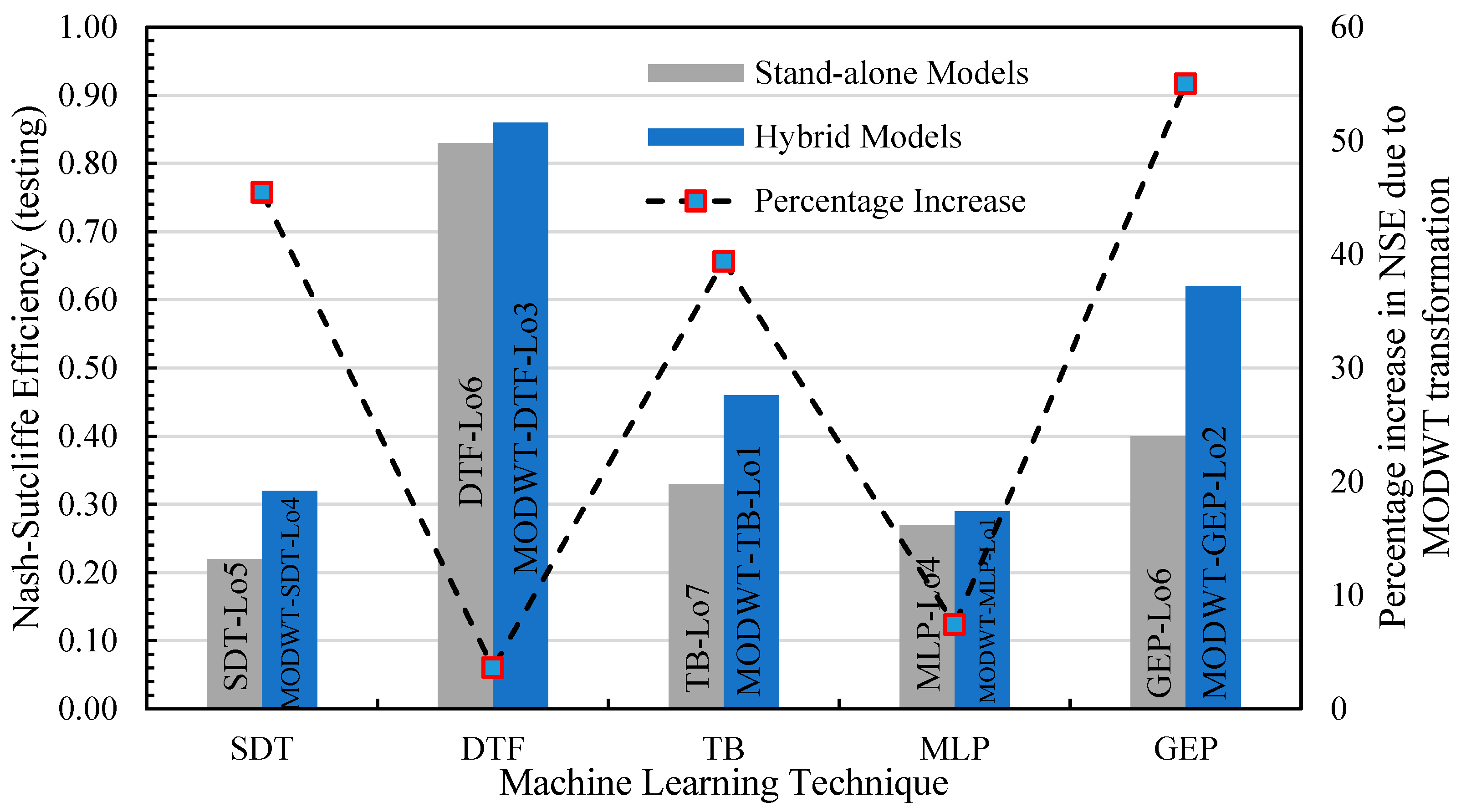
In each case, the analysis was initially run using standalone ML technique (SDT, TB, DTF, MLP, and GEP) settings and then coupled with MODWT. The findings reflected that the MODWT-based DTF model at lag order 3 (Lo3) performed best in the Bunha-Kahan River basin and at Lo4 in the Soan-Haro River basin. The modeling accuracy ranged from 0.85 to 0.90, in terms of NSE, and from 0.90 to 0.92, in terms of R². Additionally, it was proven that wavelet pre-processing improved the modeling accuracy of stand-alone machine learning models.

In the Bunha-Kahan River basin, the DTF mode, in combination with MODWT, performed best at Lo3 with an NSE value of 0.86. RMSE and R²-values were 220.45 and 0.92, respectively. The MODWT-GEP model showed the second-best performance, with an NSE value of 0.62 at Lo2, followed by an NSE value of 0.46 for the MODWT-TB model at Lo1. In the Soan-Haro River basin, the MODWT-based DTF model again performed best, with an 88% accuracy at Lo4. The MODWT-TB model recreated runoff data with 54% accuracy at lag order 2 (Lo2). The Decision Tree Forest (DTF) model performed well in each of the sub-basins when compared to standalone counter-models. When coupled with MODWT, the performance of all ML models was enhanced. However, other than the MODWT-DTF model, the modeling accuracy of SDT, TB, MLP, and GEP was generally unsatisfactory, except MODWT-GEP-Lo2 in the Bunha-Kahan River basin (NSE = 0.62).

This performance improvement is a result of the wavelet transformation’s propensity to recover latent details from the univariate time series during input signal pre-processing. Therefore, MODWT may be applied with confidence to issues requiring many variables to provide better results while using less parametric information and sparse modeling. The type, geography, and characteristics of the basin might affect the wavelet technique’s findings. Thus, it is important to choose the right wavelet family and type as well as decomposition level in order to obtain the best results.

References

1. Montanari, A.; Young, G.; Savenije, H.H.G.; Hughes, D.; Wagener, T.; Ren, L.L.; Belyaev, V. “Panta Rhei-Everything Flows”: Change in hydrology and society-The IAHS Scientific Decade 2013–2022. Hydrol. Sci. J. 2013, 58, 1256–1275. [Google Scholar] [CrossRef]
2. Ramly, S.; Tahir, W. Application of HEC-GeoHMS and HEC-HMS as Rainfall–Runoff Model for Flood Simulation. In International Symposium on Flood Research and Management [Internet]; Tahir, W., Abu Bakar, P., Wahid, M., Mohd Nasir, S., Lee, W., Eds.; Springer: Singapore, 2016. [Google Scholar] [CrossRef]
3. Masseroni, D.; Cislaghi, A.; Camici, S.; Massari, C.; Brocca, L. A reliable rainfall-runoff model for flood forecasting: Review and application to a semi-urbanized watershed at high flood risk in Italy. Hydrol. Res. 2017, 48, 726–740. [Google Scholar] [CrossRef]
4. Młyński, D.; Petroselli, A.; Wałęga, A. Flood frequency analysis by an event-based rainfall-runoff model in selected catchments of Southern Poland. Soil Water Res. 2018, 13, 170–176. [Google Scholar] [CrossRef] [Green Version]
5. Zeng, Q.; Chen, H.; Xu, C.Y.; Jie, M.X.; Hou, Y.K. Feasibility and uncertainty of using conceptual rainfallrunoff models in design flood estimation. Hydrol. Res. 2016, 47, 701–717. [Google Scholar] [CrossRef] [Green Version]
6. Talchabhadel, R.; Shakya, N.M. Rainfall Runoff Modelling for Flood. NEAJ Newsl. 2015, 1, 23–27. [Google Scholar]
7. Sharghi, E.; Nourani, V.; Najafi, H.; Molajou, A. Emotional ANN (EANN) and Wavelet-ANN (WANN) Approaches for Markovian and Seasonal Based Modeling of Rainfall-Runoff Process. Water Resour. Manag. 2018, 32, 3441–3456. [Google Scholar] [CrossRef]
8. Chau, K.W. Use of meta-heuristic techniques in rainfall-runoffmodelling. Water 2017, 9, 186. [Google Scholar] [CrossRef] [Green Version]
9. Sitterson, J.; Knightes, C.; Parmar, R.; Wolfe, K.; Avant, B. An Overview of Rainfall-Runoff Model Types An Overview of Rainfall-Runoff Model Types. In Proceedings of the 9th International Congress on Environmental Modelling and Software [Internet], Fort Collins, CO, USA, 24–28 June 2018; pp. 1–29. Available online: https://scholarsarchive.byu.edu/iemssconference/2018/Stream-C/41/?utm_source=scholarsarchive.byu.edu%2Fiemssconference%2F2018%2FStream-C%2F41&utm_medium=PDF&utm_campaign=PDFCoverPages (accessed on 17 November 2022).
10. Merabtene, T.; Kawamura, A.; Jinno, K.; Olsson, J. Risk assessment for optimal drought management of an integrated water resources system using a genetic algorithm. Hydrol. Process. 2003, 16, 2189–2208. [Google Scholar] [CrossRef]
11. Sajikumar, N.; Remya, R.S. Impact of land cover and land use change on runoff characteristics. J. Environ. Manag. 2015, 161, 460–468. [Google Scholar] [CrossRef]
12. Liu, Y.; Bralts, V.F.; Engel, B.A. Evaluating the effectiveness of management practices on hydrology and water quality at watershed scale with a rainfall-runoff model. Sci. Total Environ. 2015, 511, 298–308. [Google Scholar] [CrossRef]
13. Rezaali, M.; Quilty, J.; Karimi, A. Probabilistic urban water demand forecasting using wavelet-based machine learning models. J. Hydrol. 2021, 600, 126358. [Google Scholar] [CrossRef]
14. Fraga, I.; Cea, L.; Puertas, J. Effect of rainfall uncertainty on the performance of physically based rainfall–runoff models. Hydrol. Process. 2019, 33, 160–173. [Google Scholar] [CrossRef] [Green Version]
15. Young, C.C.; Liu, W.C.; Wu, M.C. A physically based and machine learning hybrid approach for accurate rainfall-runoff modeling during extreme typhoon events. Appl. Soft Comput. J. 2017, 53, 205–216. [Google Scholar] [CrossRef]
16. Tokar, A.S.; Johnson, P.A. Rainfall-Runoff Modeling Using Artificial Neural Networks. J. Hydrol. Eng. 1999, 4, 223–239. [Google Scholar] [CrossRef]
17. Wilby, R.L.; Abrahart, R.J.; Dawson, C.W. Detection of conceptual model rainfall-runoff processes inside an artificial neural network. Hydrol. Sci. J. 2003, 48, 163–181. [Google Scholar] [CrossRef] [Green Version]
18. Khan, M.T.; Shoaib, M.; Hammad, M.; Salahudin, H.; Ahmad, F.; Ahmad, S. Application of Machine Learning Techniques in Rainfall—Runoff Modelling of the Soan River Basin, Pakistan. Water 2021, 13, 3528. [Google Scholar] [CrossRef]
19. Okkan, U.; Ersoy, Z.B.; Ali Kumanlioglu, A.; Fistikoglu, O. Embedding machine learning techniques into a conceptual model to improve monthly runoff simulation: A nested hybrid rainfall-runoff modeling. J. Hydrol. 2021, 598, 126433. [Google Scholar] [CrossRef]
20. Poonia, V.; Tiwari, H.L. Rainfall-runoff modeling for the Hoshangabad Basin of Narmada River using artificial neural network. Arab. J. Geosci. 2020, 13, 944. [Google Scholar] [CrossRef]
21. Gomes, E.P.; Blanco, C.J.C. Daily rainfall estimates considering seasonality from a MODWT-ANN hybrid model. J. Hydrol. Hydromech. 2021, 69, 13–28. [Google Scholar] [CrossRef]
22. Nourani, V.; Tajbakhsh, A.D.; Molajou, A. Data mining based on wavelet and decision tree for rainfall-runoff simulation. Hydrol. Res. 2019, 50, 75–84. [Google Scholar] [CrossRef] [Green Version]
23. Nourani, V.; Hosseini Baghanam, A.; Adamowski, J.; Kisi, O. Applications of hybrid wavelet-Artificial Intelligence models in hydrology: A review. J Hydrol. 2014, 514, 358–377. [Google Scholar] [CrossRef]
24. Ouma, Y.O.; Cheruyot, R.; Wachera, A.N. Rainfall and runoff time-series trend analysis using LSTM recurrent neural network and wavelet neural network with satellite-based meteorological data: Case study of Nzoia hydrologic basin. Complex Intell. Syst. 2021, 8, 213–236. [Google Scholar] [CrossRef]
25. Kavoosi, M.; Khozeymehnehad, H. Review and compare performance of 4 modeling methods LS-SVM, NN, GEP and ANFIS-PSO in Simulation of Rainfall–Runoff (Study Area: Halil River—Jiroft Dam). J. Irrig. Water Eng. 2021, 11, 96–110. [Google Scholar]
26. Saifullah, M.W.M.; Hashim, S.; Shoaib, M.; Naseem, A.; Khan, M. Modelling of Rainfall-runoff process by GEP, RBF-SVM and M5 model tree in Jhelum River Basin, Pakistan. In Proceedings of the Internation Conference on Hydrology and Water Resources (ICHWR-2021), Lahore, Pakistan, 25 March 2021; pp. 105–112. [Google Scholar]
27. Asadi, S.; Shahrabi, J.; Abbaszadeh, P.; Tabanmehr, S. A new hybrid artificial neural networks for rainfall-runoff process modeling. Neurocomputing 2013, 121, 470–480. [Google Scholar] [CrossRef]
28. Okkan, U.; Serbes, Z.A. The combined use of wavelet transform and black box models in reservoir inflow modeling. J. Hydrol. Hydromech. 2013, 61, 112–119. [Google Scholar] [CrossRef] [Green Version]
29. Okkan, U. Wavelet neural network model for reservoir inflow prediction. Sci. Iran. 2012, 19, 1445–1455. [Google Scholar] [CrossRef] [Green Version]
30. Notarangelo, N.M.; Hirano, K.; Albano, R.; Sole, A. Transfer learning with convolutional neural netwoks for rainfall detection in single images. Water 2021, 13, 588. [Google Scholar] [CrossRef]
31. Van, S.P.; Le, H.M.; Thanh, D.V.; Dang, T.D.; Loc, H.H.; Anh, D.T. Deep learning convolutional neural network in rainfall-runoff modelling. J. Hydroinf. 2020, 22, 541–561. [Google Scholar] [CrossRef] [Green Version]
32. Xu, Y.; Liu, Y.; Jiang, Z.; Yang, X.; Wang, X.; Zhang, Y.; Qin, Y. Improved Convolutional Neural Network and its Application in Non-Periodical Runoff Prediction. Water Resour. Manag. 2022, 36, 6149–6168. [Google Scholar] [CrossRef]
33. Poornima, S.; Pushpalatha, M. Prediction of rainfall using intensified LSTM based recurrent Neural Network with Weighted Linear Units. Atmosphere 2019, 10, 668. [Google Scholar] [CrossRef] [Green Version]
34. Li, W.; Kiaghadi, A.; Dawson, C. High temporal resolution rainfall–runoff modeling using long-short-term-memory (LSTM) networks. Neural Comput. Appl. 2021, 33, 1261–1278. [Google Scholar] [CrossRef]
35. Luo, Q.-R.; Xu, H.; Bai, L.-H. Prediction of significant wave height in hurricane area of the Atlantic Ocean using the Bi-LSTM with attention model. Ocean Eng. 2022, 266, 112747. [Google Scholar] [CrossRef]
36. Shoaib, M.; Shamseldin, A.Y.; Khan, S.; Sultan, M.; Ahmad, F.; Sultan, T.; Dahri, Z.H.; Ali, I. Input Selection of Wavelet-Coupled Neural Network Models for Rainfall-Runoff Modelling. Water Resour. Manag. 2019, 33, 955–973. [Google Scholar] [CrossRef]
37. Shoaib, M.; Shamseldin, A.Y.; Melville, B.W. A comparison between wavelet based static and dynamic neural network approaches for runoff prediction. J. Hydrol. 2016, 535, 211–225. [Google Scholar] [CrossRef]
38. Shoaib, M.; Shamseldin, A.Y.; Melville, B.W. Comparative study of different wavelet based neural network models for rainfall-runoff modeling. J. Hydrol. 2014, 515, 47–58. [Google Scholar] [CrossRef]
39. Shoaib, M.; Shamseldin, A.Y.; Melville, B.W. Hybrid Wavelet Neural Network Approach. In Network Modelling, Studies in Computational Intelligence; Springer International Publishing: Cham, Switzerland, 2016; pp. 127–143. [Google Scholar]
40. Hammad, M.; Shoaib, M.; Salahudin, H.; Baig, M.A.I.; Khan, M.M.; Ullah, M.K. Rainfall forecasting in upper Indus basin using various artificial intelligence techniques. Stoch. Environ. Res. Risk Assess. 2021, 35, 2213–2235. [Google Scholar] [CrossRef]
41. Mahmood, G.G.; Rashid, H.; Anwar, S.; Nasir, A. Evaluation of climate change impacts on rainfall patterns in pothohar region of pakistan. Water Conserv. Manag. 2019, 3, 1–6. [Google Scholar] [CrossRef]
42. Tallat, Q.; Siddiqui, M.; Hashmi, H.N.; Ghumman, A.R. Runoff Modeling for a Watershed in Pothowar Region of Pakistan. Mehran Univ. Res. J. Eng. Technol. 2012, 31, 379–394. [Google Scholar]
43. Siddiqui, Q.T.M.; Hashmi, H.N.; Mughal, H.R. Development of Small Dams in Pothowar Plateu of Punjab (Pakistan). In Proceedings of the ICID 21st International Congress on Irrigation and Drainage, Tehran, Iran, 15–23 October 2011; pp. 121–129. [Google Scholar]
44. Breiman, L. Arcing the Edge; University of California: Berkeley, CA, USA, 1998. [Google Scholar]
45. Breiman, L. Random forests. Mach. Learn. 2001, 45, 5–32. [Google Scholar] [CrossRef] [Green Version]
46. Raza, A.; Shoaib, M.; Khan, A.; Baig, F.; Faiz, M.A.; Khan, M.M. Application of non-conventional soft computing approaches for estimation of reference evapotranspiration in various climatic regions. Theor. Appl. Climatol. 2020, 139, 1459–1477. [Google Scholar] [CrossRef]
47. Webros, P.J. Beyond Regression: New Tools for Prediction and Analysis in the Behavioral Sciences; Harvard University: Cambridge, MA, USA, 1974. [Google Scholar]
48. Goodfellow, I.; Bengio, Y.; Courville, A. Deep Learning; MIT Press: Cambridge, MA, USA, 2016. [Google Scholar]
49. Ferreira, C. Gene Expression Programming: A New Adaptive Algorithm for Solving Problems. Complex Syst. 2001, 13, 87–129. [Google Scholar]
50. Percival, D.B.; Walden, A.T. The Maximal Overlap Discrete Wavelet Transform. In Wavelet Methods for Time Series Analysis; Cambridge University Press: Cambridge, UK, 2000; pp. 159–205. [Google Scholar]
51. Quilty, J.; Adamowski, J. Addressing the incorrect usage of wavelet-based hydrological and water resources forecasting models for real-world applications with best practices and a new forecasting framework. J. Hydrol. 2018, 563, 336–353. [Google Scholar] [CrossRef]
52. Walden, A.T. Wavelet Analysis of Discrete Time Series. Eur. Congr. Math. 2001, 2, 627–641. [Google Scholar]
53. Ramana, R.V. Monthly Rainfall Prediction Using Wavelet Neural Network Analysis. Water Resour. Manag. 2013, 27, 3697–3711. [Google Scholar] [CrossRef] [Green Version]
54. May, R.J.; Dandy, G.C.; Maier, H.R.; Nixon, J.B. Application of partial mutual information variable selection to ANN forecasting of water quality in water distribution systems. Environ. Model. Softw. 2008, 23, 1289–1299. [Google Scholar] [CrossRef]
55. Ribeiro, G.H.T.; De Neto, P.S.G.M.; Cavalcanti, G.D.C.; Tsang, I.R. Lag selection for time series forecasting using Particle Swarm Optimization. In Proceedings of the International Joint Conference on Neural Networks, San Jose, CA, USA, 31 July–5 August 2011; pp. 2437–2444. [Google Scholar]
56. Maheswaran, R.; Khosa, R. Comparative study of different wavelets for hydrologic forecasting. Comput. Geosci. 2012, 46, 284–295. [Google Scholar] [CrossRef]
57. Nash, J.E.; Sutcliffe, J.V. River Flow Forecasting Through Conceptual Models Part I—A Disclission of Principles*. J. Hydrol. 1970, 10, 282–290. [Google Scholar] [CrossRef]
58. Hussain, F.; Wu, R.; Nabi, G.; Hussain, B. A Study on Rainfall, Runoff and Sediment Yield Relations in Small Watersheds of Pothwar Region Pakistan. In Proceedings of the 2017 Conference on Sustainable Development for Environmental Resources, Taiwan, 24–26 November 2017. [Google Scholar]
59. Ghani, M.W.; Arshad, M.; Shabbir, A.; Shakoor, A.; Mehmood, N.; Ahmad, I. Investigation of potential water harvesting sites at potohar using modeling approach. Pakistan J. Agric. Sci. 2013, 50, 723–729. [Google Scholar]
60. Jhong, Y.D.; Chen, C.S.; Lin, H.P.; Chen, S.T. Physical hybrid neural network model to forecast typhoon floods. Water 2018, 10, 632. [Google Scholar] [CrossRef] [Green Version]
61. Song, Y.Y.; Lu, Y. Decision tree methods: Applications for classification and prediction. Shanghai Arch. Psychiatry 2015, 27, 130–135. [Google Scholar]
62. Lin, N.; Noe, D.; He, X. Tree-based methods and their applications. In Springer Handbook of Engineering Statistics, 49th ed.; Pham, H., Ed.; Springer: London, UK, 2006; pp. 551–570. [Google Scholar]
63. Danial Mohammadzadeh, S.; Kazemi, S.F.; Mosavi, A.; Nasseralshariati, E.; Tah, J.H.M. Prediction of compression index of fine-grained soils using a gene expression programming model. Infrastructures 2019, 4, 26. [Google Scholar] [CrossRef] [Green Version]
64. Tu, J.V. Advantages and disadvantages of using artificial neural networks versus logistic regression for predicting medical outcomes. J. Clin. Epidemiol. 1996, 49, 1225–1231. [Google Scholar] [CrossRef]
65. Adamowski, J.; Sun, K. Development of a coupled wavelet transform and neural network method for flow forecasting of non-perennial rivers in semi-arid watersheds. J. Hydrol. 2010, 390, 85–91. [Google Scholar] [CrossRef]
Figure 1. Location map of river basins within the Pothohar Region.
Atmosphere 14 00452 g001
Figure 7. Graphical illustration of detail components (at level 1, 2, and 3) and approximation component at level 3 for rainfall timeseries of the Soan-Haro River basin.
Atmosphere 14 00452 g007
Figure 8. Training NSE score of stand-alone machine learning models in Bunha-Kahan River basin.
Atmosphere 14 00452 g008
Figure 9. Testing NSE score of stand-alone machine learning models in Bunha-Kahan River basin.
Atmosphere 14 00452 g009
Figure 10. Training NSE score of hybrid machine learning models in Bunha-Kahan River basin.
Atmosphere 14 00452 g010
Figure 11. Testing NSE score of hybrid machine learning models in Bunha-Kahan River basin.
Atmosphere 14 00452 g011
Figure 12. Comparative analysis of best performing models of stand-alone ML techniques in Bunha-Kahan River basin.
Atmosphere 14 00452 g012
Figure 13. Comparative analysis of best performing models of stand-alone and MODWT-hybrid techniques in Bunha-Kahan River basin.
Atmosphere 14 00452 g013
Figure 14. Comparative analysis of best models in Bunha-Kahan River basin.
Atmosphere 14 00452 g014
Figure 15. Regression plot (MODWT-DTF-Lo3) in Bunha-Kahan River basin.
Atmosphere 14 00452 g015
Figure 16. Rainfall-Runoff modeling of Bunha-Kahan River basin (MODWT-DTF-Lo3).
Atmosphere 14 00452 g016
Figure 17. NSE score of stand-alone machine learning models in training in the Soan-Haro River basin.
Atmosphere 14 00452 g017
Figure 18. NSE score of stand-alone machine learning models in testing in the Soan-Haro River basin.
Atmosphere 14 00452 g018
Figure 19. NSE score of hybrid machine learning models in training in the Soan-Haro River basin.
Atmosphere 14 00452 g019
Figure 20. NSE score of hybrid machine learning models in testing in the Soan-Haro River basin.
Atmosphere 14 00452 g020
Figure 21. Comparative analysis of best performing models of stand-alone ML techniques in the Soan-Haro River basin.
Atmosphere 14 00452 g021
Figure 22. Comparative analysis of best performing models of stand-alone and MODWT-hybrid techniques in the Soan-Haro River basin.
Atmosphere 14 00452 g022
Figure 23. Comparative analysis of best models in the Soan-Haro River basin.
Atmosphere 14 00452 g023
Figure 24. Regression plot (MODWT-DTF-Lo4) in the Soan-Haro River basin.
Atmosphere 14 00452 g024
Figure 25. Rainfall-Runoff Modeling of the Soan-Haro River basin (MODWT-DTF-Lo4).
Atmosphere 14 00452 g025