

Synthetic Drought Hydrograph
1
Department of Hydrotechnical Engineering, Technical University of Civil Engineering of Bucharest, 020396 Bucharest, Romania
2
Roua Soft SRL, 040271 Bucharest, Romania
3
Urban Arte Studio, 021177 Bucharest, Romania
*
Author to whom correspondence should be addressed.
Hydrology 2023, 10(1), 10; https://doi.org/10.3390/hydrology10010010
Submission received: 24 November 2022
/
Revised: 20 December 2022
/
Accepted: 25 December 2022
/
Published: 30 December 2022
(This article belongs to the Special Issue Stochastic and Deterministic Modelling of Hydrologic Variables)
Abstract
:Droughts are natural disasters with a significant impact on the economy and social life. Prolonged droughts can cause even more damage than floods. The novelty of this work lies in the definition of a synthetic drought hydrograph (SDH) which can be derived at each gaging station of a river network. Based on drought hydrographs (DHs) recorded for a selected gaging station, the SDH is statistically characterized and provides valuable information to water managers regarding available water resources during the drought period. The following parameters of the registered drought hydrograph (DH) are proposed: minimum drought discharge , drought duration and deficit volume . All these parameters depend on the drought threshold , which is chosen based on either pure hydrological considerations or on socio-economic consequences. For the same statistical parameters of the drought, different shapes of the synthetic drought hydrograph (SDH) can be considered. In addition, the SDH varies according to the probabilities of exceedance of the minimum drought discharge and deficit volume.
1. Introduction
Drought is a situation characterized by the lack of sufficient water resources to meet the demands of plants, animals and human populations, their lifestyles and land use [1]. The main cause of drought is the lack of precipitation in combination with hot temperature and evapotranspiration values [2]. Excessive abstraction or inadequate management of water resources can worsen drought problems. Drought can be classified as meteorological drought, soil moisture drought, hydrological drought, and socio-economic drought [3,4,5]. Pedological drought is a consequence of meteorological drought, while hydrological drought (including its effects on groundwater resources) is the result of pedological drought. Although hydrological drought is a consequence of meteorological drought, the lag time between meteorological input to the hydrological system and the occurrence of deficiencies in surface and groundwater resources can be considerable [5,6,7]. For this reason, meteorological drought can be a warning of future hydrological drought. Socio-economic drought differs significantly from other types of droughts because it reflects the relationship between water demand and available water resources that varies annually depending on the rainfall regime [6].
Hydrological drought is defined by the insufficient amount of surface and subsurface water resources compared to average conditions in space and in time across seasons [4,6,8] and manifests itself at the level of all forms of water circulation in the terrestrial phase [9]. Streamflow is the best indicator of hydrological drought [10] because it integrates surface runoff, subsurface runoff from unsaturated zones and base flow from aquifers.
For the study of low flows there are two approaches: (a) the minimum annual n-day discharge and (b) deficits below a certain threshold [5,7]. These approaches characterize local-scale events [11], leading to a “local fingerprint” of drought from daily hydrographs [12].
In this paper, hydrological drought was considered to represent a deficiency of river flow below a predefined threshold [13]. Consequently, the truncation level (threshold) should be determined to define drought characteristics [5,14]. Below the threshold, river flow is in deficit [5].
The Czech Hydro-Meteorological Study considers a drought event if the discharge falls below Q355, while [12] considered as a low-flow event all discharges below the annual threshold Q80. Thresholds used to define low-flow events are typically in the 70–95th percentile range [5,14,15].
Attention during drought is usually focused on agricultural drought because of the consequences for food security. There are also concerns during hydrological drought concerning cooling water for nuclear reactors, safe water levels for navigation or necessary discharge for hydroelectricity production. During periods of drought, other water users are also affected, such as the population, industry, or the environment. Water managers face the problem of water allocation under uncertainties related to the evolution of the drought. Their water allocation decisions are usually based on the 90th percentile flow (Q90), being the discharge exceeded on average 90% of the time or 328 days per year [2]. In other words, Q90 is considered an indicator of socio-economic drought.
There are similarities between the flood hydrograph and the drought hydrograph, the former being above a certain threshold (standing for the base flow), while the latter is computed below another threshold, much lower than for floods. The drought threshold is chosen based on hydrological considerations as shown above or is defined according to socio-economic drought, represented by the minimum discharge for essential water users (including environmental flow).
The threshold level method, which studies runs below or above a given threshold and originally termed ‘method of crossing theory’, was introduced by Yevjevich in 1967 [5]. The use of the threshold leads to a partial duration series, which in the case of floods is known as POT (peak over threshold) [16,17,18,19,20]. In the case of drought, the similar approach could be called VBT (value below threshold).
The duration of the drought corresponds to a continuous sequence of river flow deficits. The cumulative deficit below the threshold during the drought duration is known as drought severity. The average value of individual deficits during the drought episode (the average deficit) represents the drought intensity or drought magnitude, which is defined as the ratio of drought deficit volume to duration [20].
Hydrological Drought Parameters
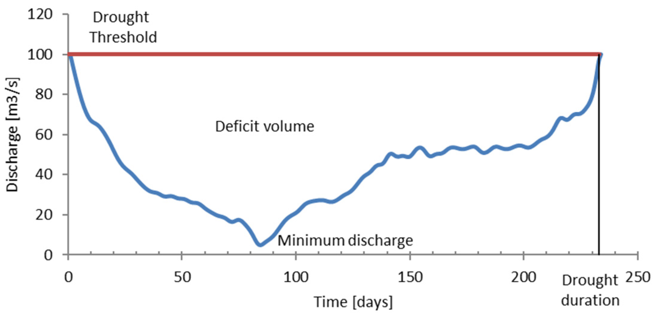
Considering the parameters proposed by different authors [5,11,21,22], the main parameters chosen to characterize the drought hydrograph (or the deficits hydrograph) are drought threshold , drought minimum discharge , time corresponding to minimum discharge, drought duration and deficit volume below the drought threshold (Figure 1).
Except for the drought threshold, the other parameters are calculated according to the following equations:
The drought duration represents the maximum value of time for which is continuously below . The minimum discharge during is . Finally, the deficit volume (or cumulative deficit) is the area between the drought hydrograph during the duration and the threshold .
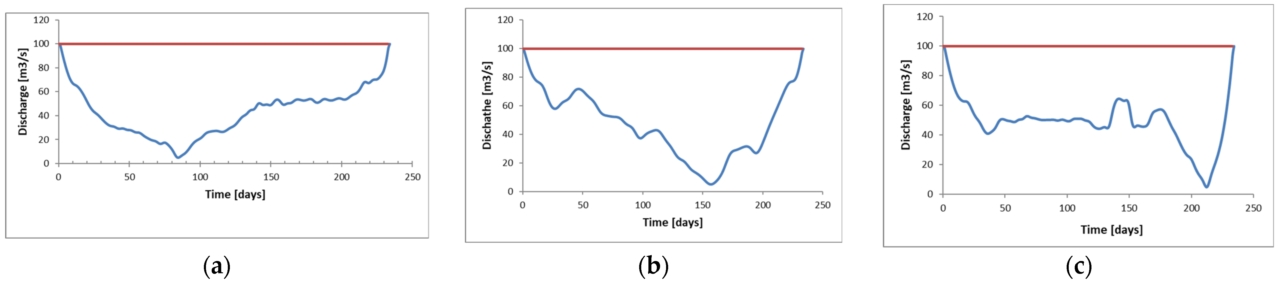
These parameters define characteristic points of the drought hydrograph. This means that any drought hydrograph must pass through the points of coordinates: . However, there are an infinite number of U-shaped curves, monotonic or not, that pass through the points that necessarily belong to the drought hydrograph. To obtain a unique solution it is necessary to introduce the shape of the drought hydrograph as a qualitative parameter of the DH. Examples of drought shapes (from the infinite number of U-shaped drought hydrographs) considering the same drought duration, minimum discharge and deficit volume are shown below (Figure 2).
The novelty of this work lies in the definition of a synthetic drought hydrograph, which can be developed not only for surface water but also for groundwater. While for surface water the drought hydrograph refers to discharges, for groundwater the drought hydrograph refers to water levels. The drought hydrograph is of particular interest for water management under water scarcity conditions, especially if the extent of the drought is forecasted based on the size of the meteorological drought.
2. Materials and Methods
Daily flows are used to find drought characteristics. It was noticed that there is a good correlation between and , which means that only and should be analyzed statistically. Based mainly on these parameters, the hydrological or hydrogeological SDH is statistically defined and can be provided to water managers.
A preliminary step is to obtain the pair of statistical values and of the SDH, which can be derived in two ways:
(a) The statistical series of and of the registered droughts are processed independently. In the following, the worst-case scenarios must be found. Such a scenario assumes a realistic or acceptable minimum flow (i.e., has a high probability of exceedance), while the deficit volume is as high as possible (so it corresponds to a low exceedance probability). Let P1% be the probability of exceedance of the minimum flow and P2% be the probability of exceedance of the deficit volume. For example, if P1% is 95%, this means that, on average, in 95 years out of 100, the minimum flow is greater than , as well as, on average, in 5 years out of 100, the minimum flow is less than . Similarly, if P2% is 10%, on average in 10 years out of 100, the deficit volume is greater than . Consequently, the pair () is used for the SDH calculation. If the selected pair is a more severe drought is considered because and .
(b) Using bivariate frequency analysis of minimum discharges and the corresponding deficit volume. Minimum discharges and deficit volumes are usually not independent variables, although their correlation coefficient might be quite low. Another option is to use copulas that overcome the disadvantages of bivariate distributions [23,24]. In each case, a family of contour lines for the P% probabilities are obtained:
where P% can be 0.1%, 1%, 10%, 20% or any other value corresponding to the drought whose magnitude can be exceeded for more than 1000, 100, 10, 5 years etc. The contour lines for each probability highlight an infinite number of pairs (minimum discharge, deficit volume), from which a selection of the most critical combinations should be made.
2.1. Threshold Selection
For the statistical processing of minimum discharges and corresponding deficit volumes, only values below a threshold are of interest. The threshold may be fixed or variable [5,14]. A fixed threshold is a constant value used for the entire series and can be chosen so that the number of droughts selected is equal to the number of years with registered discharges. Thus, the empirical probability associated with values can be interpreted as an annual probability of exceedance [25]. If not, the resulting exceedance probabilities should be converted to annual exceedance probabilities [26]. However, these additional calculations are not necessary if the number of selected droughts is equal to the number of years with registered values.
Choosing the threshold is an iterative process. A threshold discharge value is proposed, and the corresponding drought hydrographs are selected. If the number of drought periods thus obtained is less than the number of years with recorded data, the threshold is increased until equality is reached. If, on the contrary, the number of resulting drought hydrographs is greater than the number of years, the threshold value is lowered. It should also be considered that the time interval between two drought periods should be at least 1 month, and the length of the drought should be at least 1 week.
2.2. Minimum Discharges
Following the choice of the threshold , the minimum discharges for each selected drought period are processed. For partial-duration series the following distributions are preferred: Gumbel, Lognormal, Pearson type III and Pearson type V [27], the three parameter Weibull, the log-Pearson type III and the two-parameter and three-parameter lognormal distributions [28], Log-normal, Log-Pearson III, Weibull or Fréchet [29] and the two-parameter gamma and Weibull distributions [30]. In addition, other statistical distributions can be used [31]: Log Logistic, Fatigue Life, Inverse Gaussian, Johnson SB and Generalized Extreme. Different statistical tests are used for ranking the statistical distribution. In each case, graphs are plotted on normal probability paper, allowing a better visualization of the cumulative distribution function especially for small or large probabilities of exceedance.
2.3. Deficit Volumes
As with minimum discharges, the partial series of the droughts’ volume is also processed based on the VBT approach. Given the threshold discharge , all droughts whose discharges are below this threshold are selected.
The deficit volume is calculated based on the Equation (3). Satisfactory results were obtained using the following statistical distributions: Phased-Bi-Weibull, Beta, Wakeby and Log-Logistic [14].
2.4. Shape of the Drought Hydrograph
The shape of SDHs reproduces the shape of DHs that have occurred in the past, considering either the shape of the hydrograph registered during an exceptional drought, or an average shape of drought hydrographs with similar shapes. Three examples of drought shapes are shown in Figure 2.
To obtain the SDH shape, all drought hydrographs below the threshold are normalized and grouped into classes of similar shape. A class holds one or more DHs with similar shape. If a class has only one DH, it models that class.
The normalized drought hydrographs, defined by the coordinates are dimensionless and have the same shape as the original droughts. The maximum values on both axes are 100%:
At the same time:
The average dimensionless hydrograph of a class is obtained by considering the dimensionless hydrographs belonging to the same class, weighted by the following factor:
where:
—weighting factor for the dimensionless drought [–].
—minimum discharge of drought [m3/s].
—number of dimensionless droughts belonging to the same class [–].
In the following, the weighted average drought in class is given by the following equation:
where:
is the dimensionless discharge of the drought belonging to class .
When (only one DH belongs to the class ), the Equation (10) becomes:
2.5. Compactness Coefficient of the Drought Hydrograph
To exclude non-significant droughts, only the first droughts in ascending order of minimum flow are kept before calculating the compactness coefficient. A recommended value for is .
The compactness coefficient is the ratio between the deficit volume and the area of the rectangle that surrounds the deficits hydrograph:
The compactness coefficients are calculated for all dimensionless droughts. The dimensionless time corresponding to the minimum discharge of the normalized floods is also found.
2.6. Duration of the SDH
According to Equation (12), the drought duration is:
where:
is the deficit volume below the threshold ;
—the compactness coefficient of the drought;
—minimum discharge during the drought period;
—the threshold value;
The drought duration depends on the probabilities associated to drought discharge and deficit volume and can be written as follows:
The duration has a variable size, depending on the probabilities and of the minimum discharge and of the deficit volume, respectively, as well as the values of the compactness coefficient.
2.7. Construction of SDH
The ordinates of SDH represent a weighted sum (or a convex combination) of the threshold and minimum discharge . The time in days on the abscissa is obtained by multiplying the dimensionless time by the flood duration . Thus, SDH is obtained with the following equations:
where are the SDH coordinates. The resulting SDHs reproduce the average shape of significant droughts that have occurred in the past. The SDHs in each class are characterized by the same parameters: , but the shape and time to minimum discharge are different.
3. Case Study
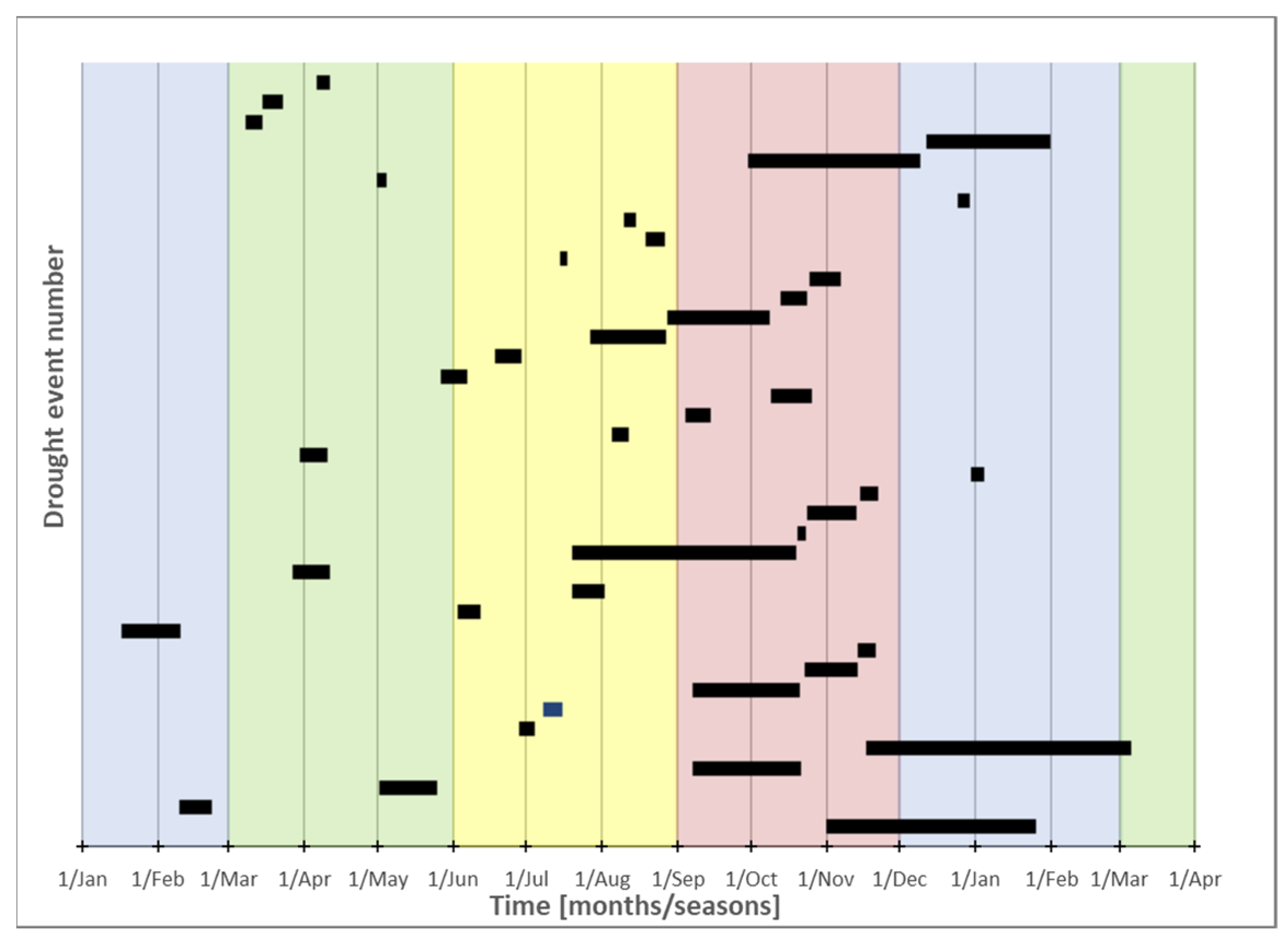
The complete time series of daily discharges registered the at Lungoci on Siret River from 1970 to 2008 was available for statistical analysis. The Lungoci gaging station is located at the lower end of the Siret River and was chosen for analysis because it characterizes the availability of water resources throughout the whole river basin. The river basin upstream of the Lungoci station has an area of over 40,000 km2 and the average flow rate is 220 m3/s. The threshold equal to 66 m3/s, was obtained by trial and error so that the number of droughts selected equals the number of years with records. The minimum discharge for the whole period is in the range of 15.6–33.8 m3/s, while the deficit volume is between 10 and 540 mil. m3. The duration of the drought for the chosen threshold is in the range of 10–109 days. Drought period can occur not only in summer and winter but also in spring or autumn or can be inter-annual (Figure 3).
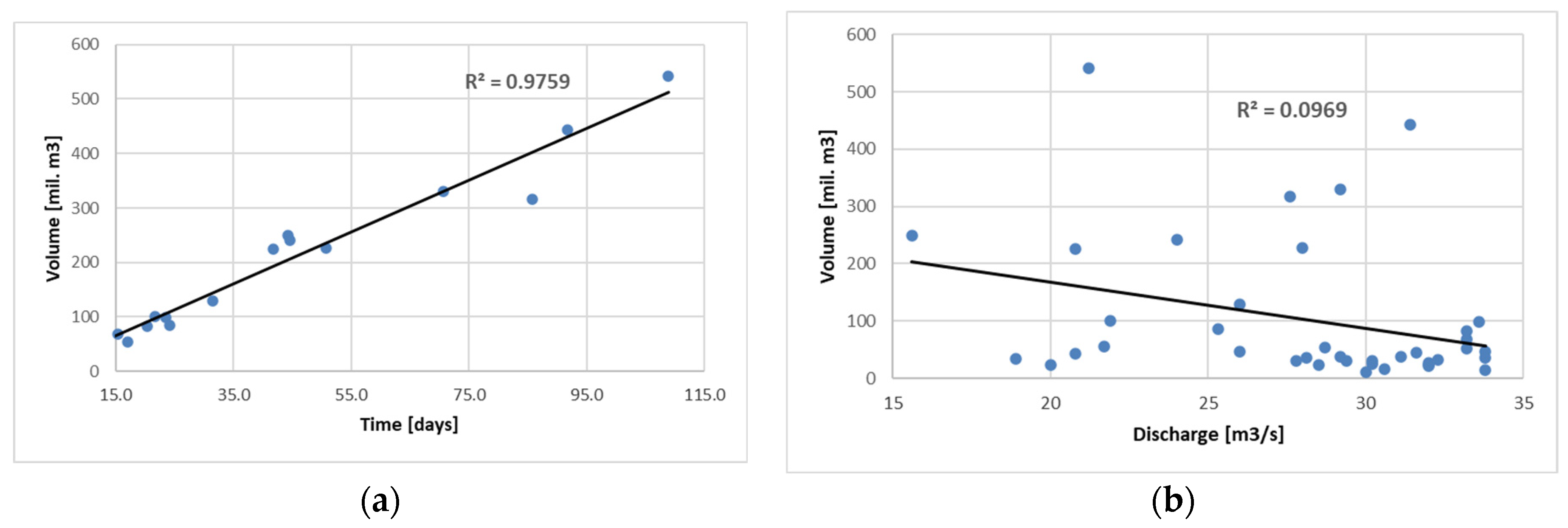
There is a good correlation (Figure 4a) between drought duration and deficit volume (R2 = 0.9645), while the correlation between minimum discharge and deficit volume (Figure 4b) is low (R2 = 0.0969), meaning the minimum discharge and deficit volume are not linearly correlated. For this reason, a bi-variate or copula analysis are not justified.
Minimum drought discharges and deficit volumes were statistically tested. According to the statistical tests, in all cases the null hypothesis (mutual independence, mutual homogeneity and lack of trend) is accepted at the threshold of 10%.
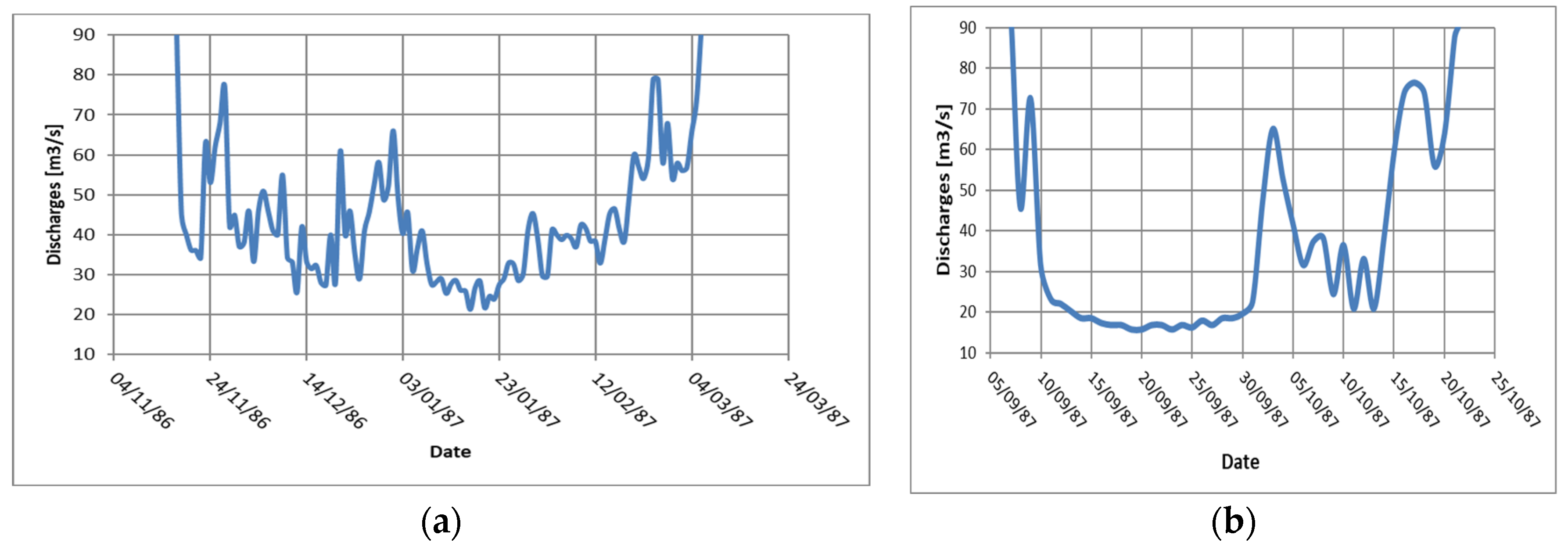
Two registered drought hydrographs are represented in Figure 4: a hydrograph of maximum duration and largest deficit volume (109 days and 542 mil. m3—Figure 5a), and another hydrograph corresponding to the minimum discharge (15.6 m3/s—Figure 5b). The two hydrographs are not monotonic and sometimes show sudden increases in discharge that can be explained by the contribution of sub-catchments where rainfall occurred.
3.1. Minimum Drought Discharges
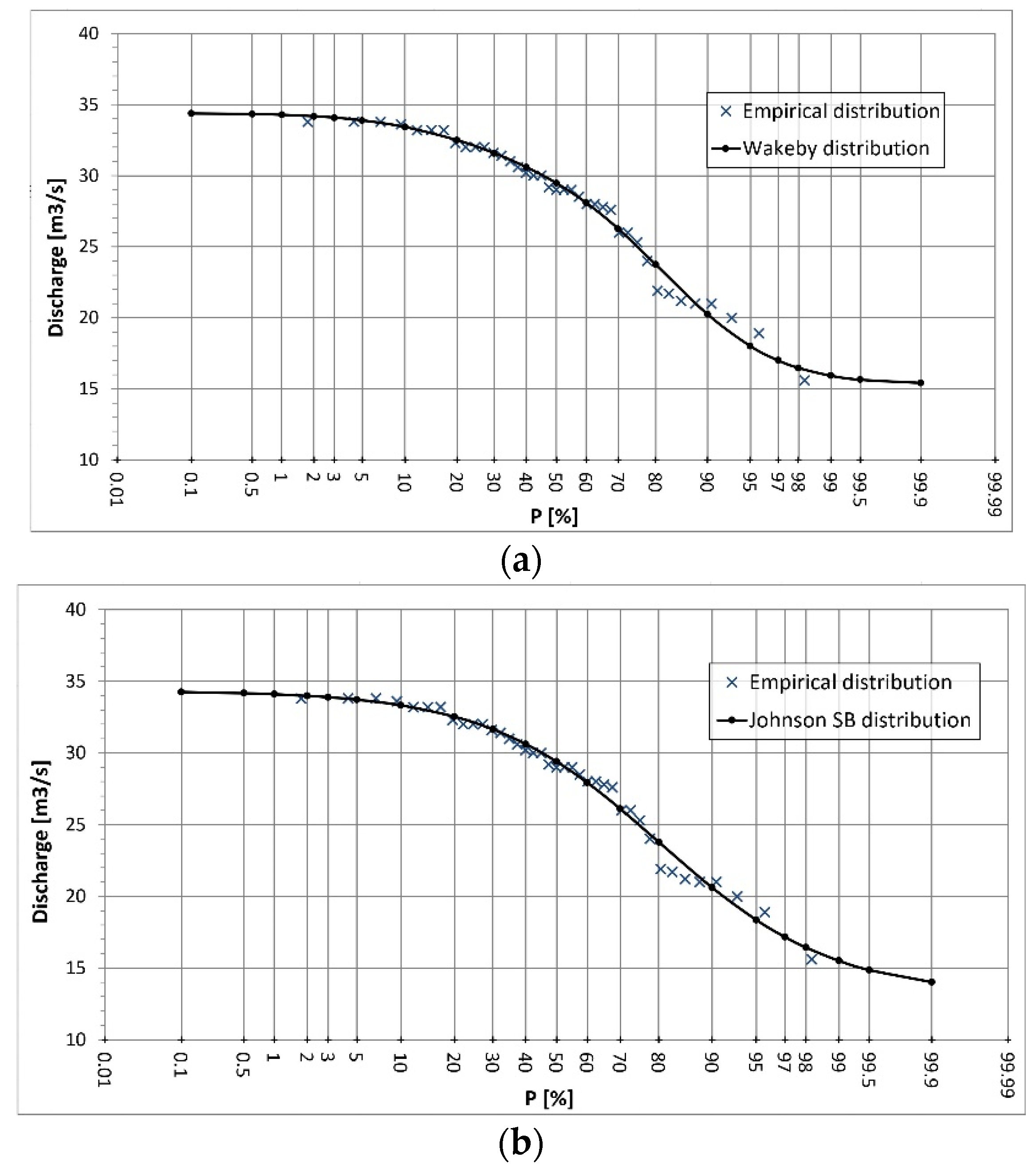
Different statistical distributions were analysed. The Wakeby and Johnson SB distributions, ranked on the top two positions according to the Kolmogorov–Smirnov test, also meet the graphical criteria (Figure 6).
The parameters of the two distributions are the following: Wakeby (46.688; 4.7786; 8.4856; −0.96137; 15.361) and Johnson SB (−0.84718; 0.71126; 21.184; 13.159).
The minimum discharges of the two distributions for the usual probabilities of exceedance are shown in Table 1. Except for low probabilities of exceedance, the two distributions are close to each other.
3.2. Deficit Volumes
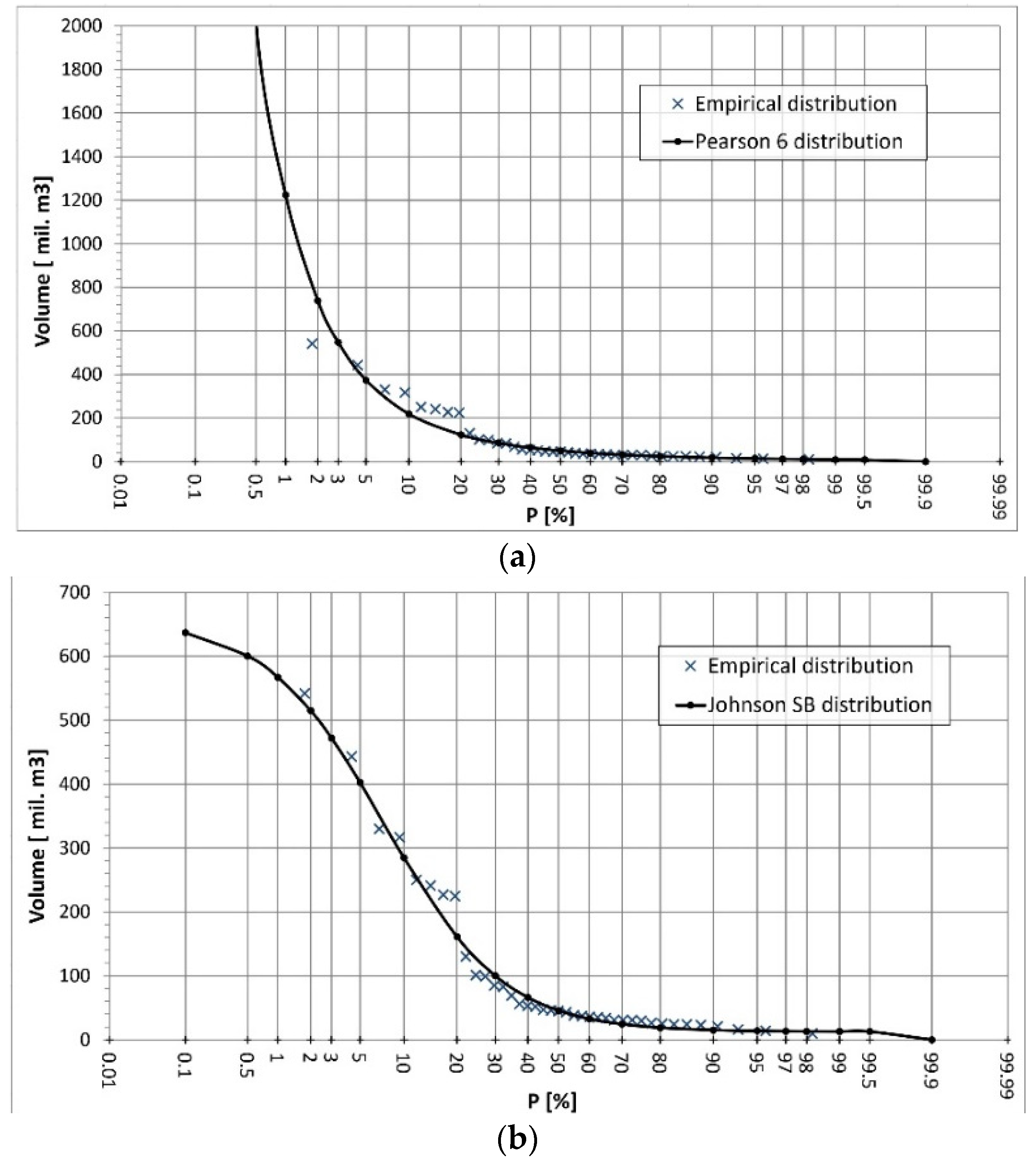
The deficit volume for each selected period was calculated using Equation (3). The results obtained for the Pearson 6 and Johnson SB distributions are shown in Figure 7 and Table 2. Unlike the distributions for minimum discharges (Figure 6), the distributions for deficit volumes (Figure 7) differ widely, especially for medium and low probabilities of exceedance.
The Pearson 6 distribution takes values in the range (7; 6386) mil.m3, while the Johnson distribution has a much narrower range of values (13; 637) mil.m3. It should be noted, however, that the Pearson 6 distribution is much better ranked according to the Kolmogorov–Smirnov test. Goodness of fit tests respond well to analysis of current droughts but provide an inconsistent fit for low probabilities of exceedance. This suggests that the statistical criteria must be additionally accompanied by a graphical and plausibility assessment based on expert judgement of the drought deficit and its duration.
3.3. Shape of the DH
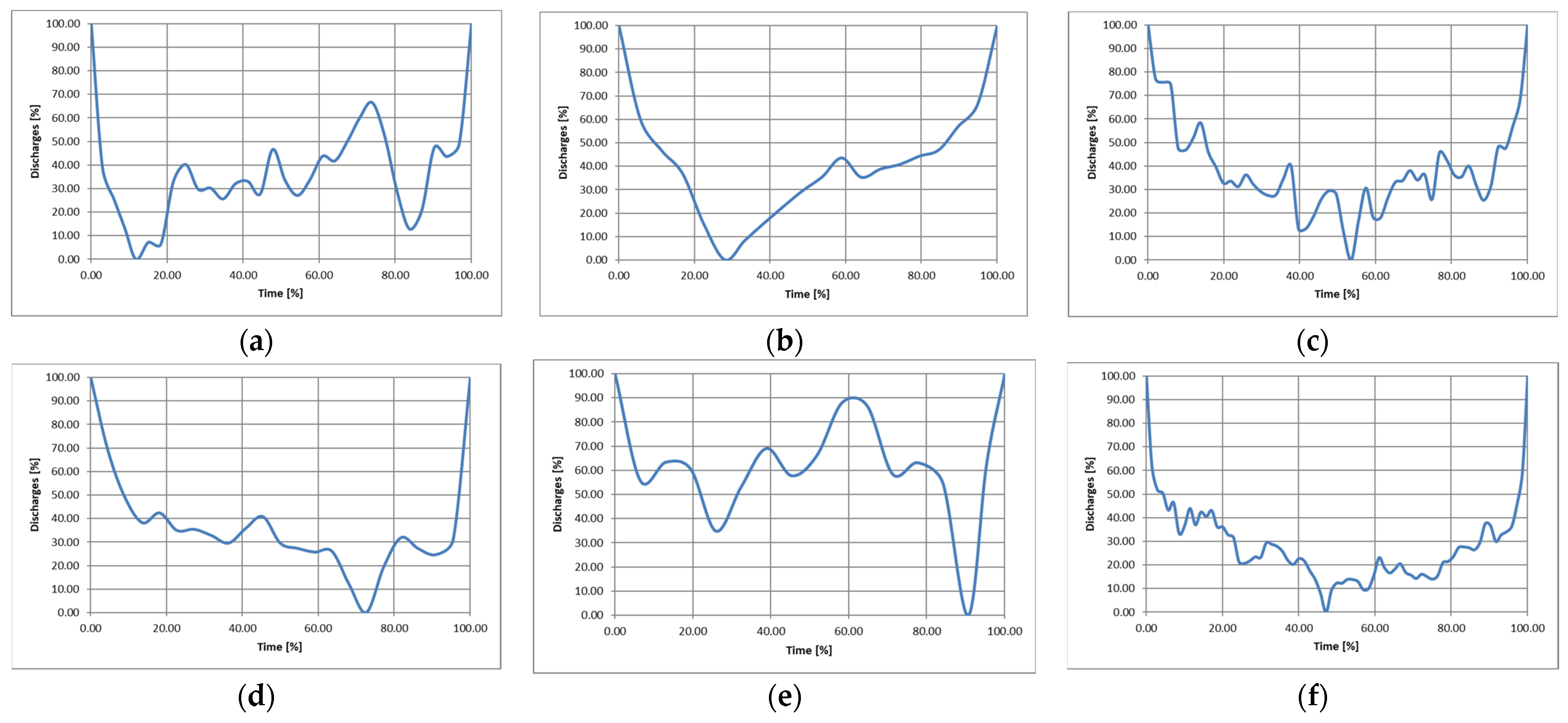
According to their shape, the DHs were grouped into six classes (Figure 8).
The dimensionless droughts in classes 3, 4 and 6 have the highest coefficients of compactness. For this reason, SDHs were determined only for these classes.
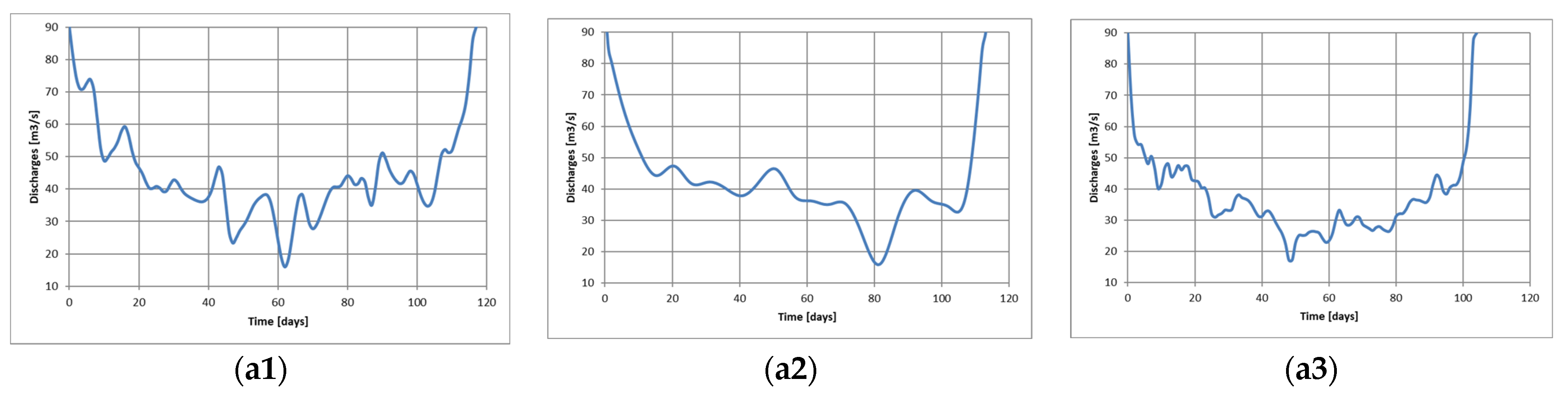
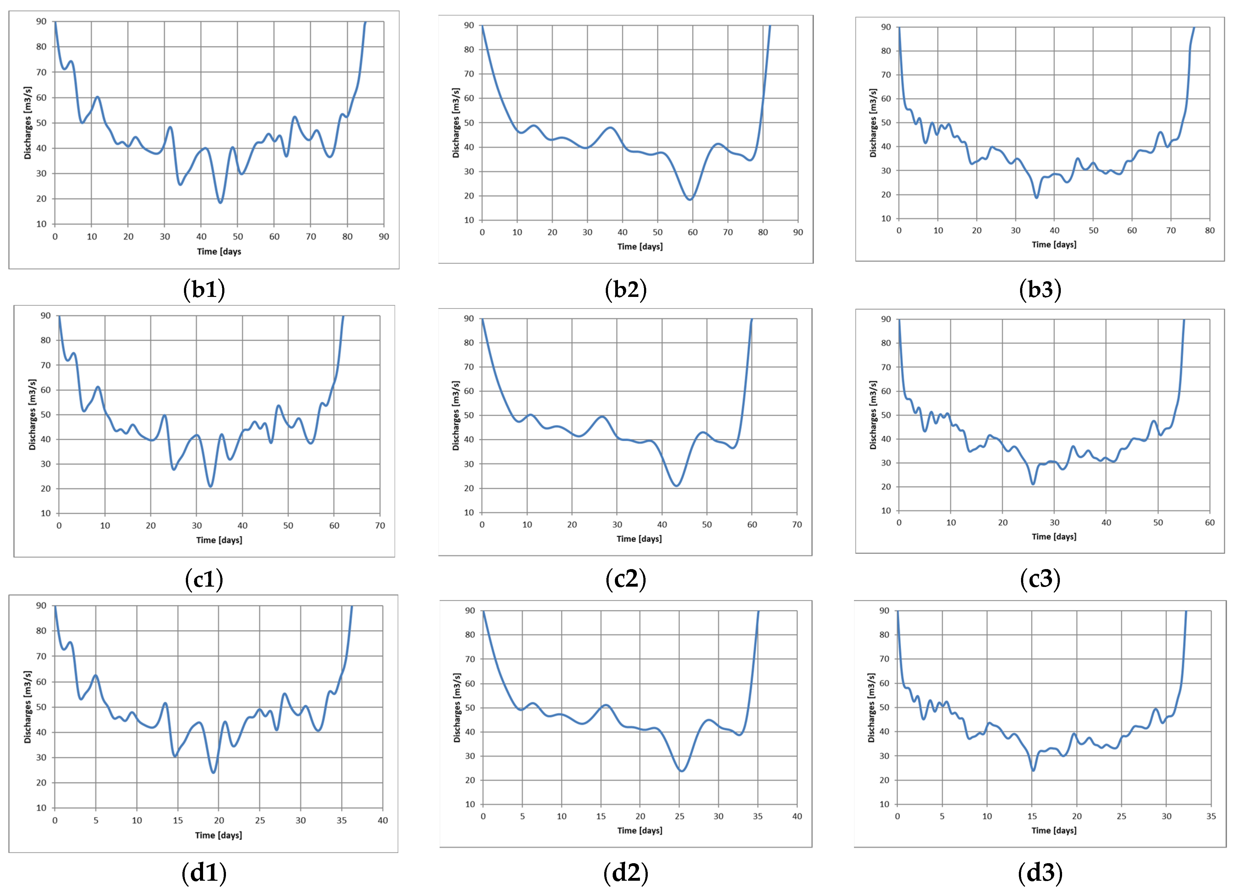
Figure 9 shows the SDHs obtained for the following pairs of parameters: (a) ; ; (b) ; ; (c) ; ; (d) ; . Both the values for minimum discharges and the values for deficit volumes correspond to the Johnson SB distribution. The main parameters of SDHs are provided in Table 3.
In the following, the Johnson distribution is considered for minimum discharges, while the distribution Pearson 6 is used for processing the deficit volumes. Given the high uncertainty of the deficit volumes for the exceedance probability 0.1% (Table 2), volume data are considered for exceedance probabilities of less than 1%.
The corresponding parameters are provided in Table 4.
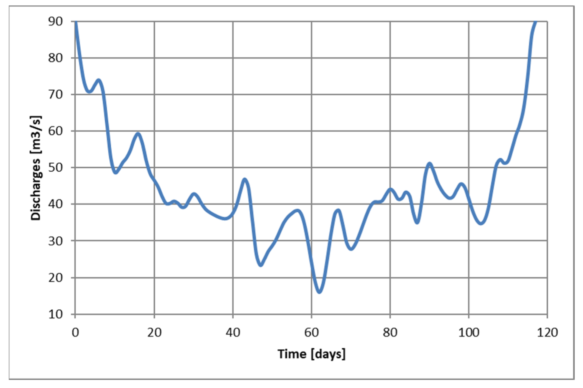
Note the extremely long duration of SDH for the pair of parameters , which can characterize an interannual drought. The wide range of values obtained for the volume deficit as well as for the duration of the drought with the Johnson SB distribution (Table 3) and Pearson 6 distribution (Table 4) highlights a high uncertainty. The SDH obtained for the probabilities of exceedance (99%; 1%) is shown in Figure 10.
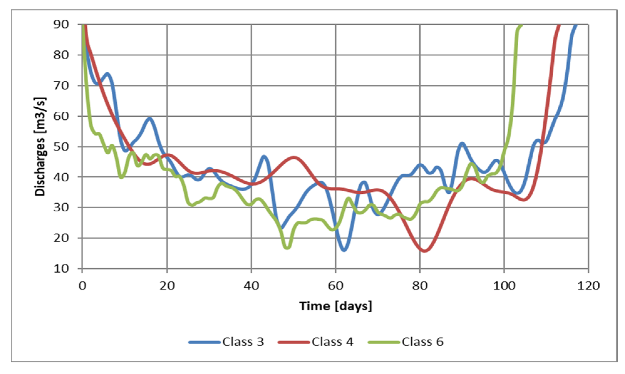
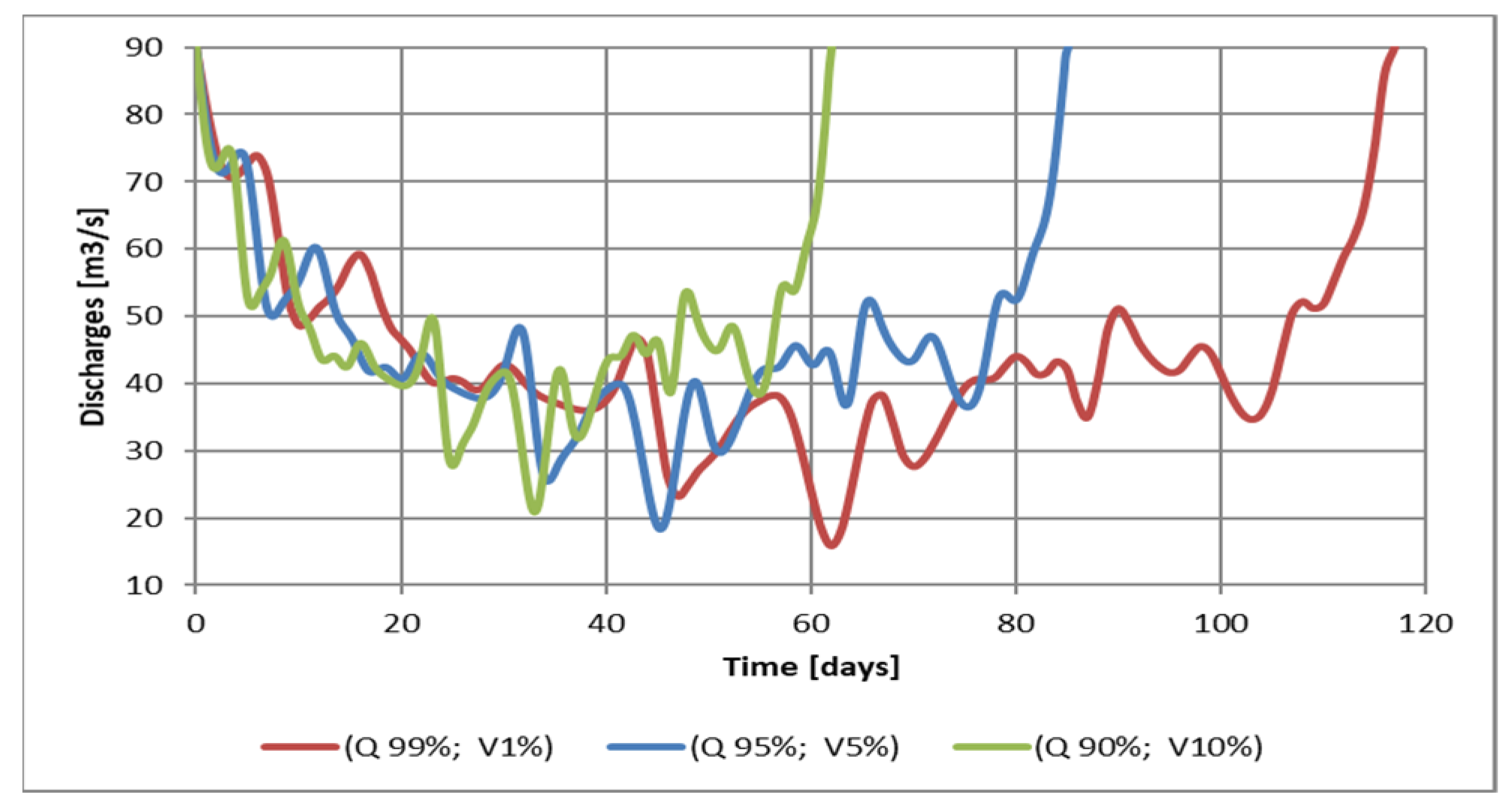
Droughts corresponding to the same pair of probabilities of exceedance and the same distributions for the minimum discharge and deficit volume, respectively, differ not only in their shape but also in their duration (Table 3). For example, the drought ( has a duration of 116, 112 or 103 days for class 3, 4 and 6, respectively (Figure 11). However, their minimum discharge and deficit volume are the same.
4. Discussion
1. The SDH is a new concept in understanding the hydrological drought behaviour. Different authors have focused on finding drought characteristics such as duration, intensity, and severity. An excellent synthesis of earlier research can be found in [14]. Drought severity and duration have been studied based on multivariate theory. The development of drought iso-severity curves for specific return periods and durations is another research direction. Other studies are oriented towards methodologies for obtaining drought return periods. In this paper, hydrologic drought is treated as a multi-variate event, which apart from its duration, intensity, and severity is also characterized by its shape. A statistically characterized complete drought hydrograph is useful in pre-drought crisis decision-making, leading to the adoption of structural and non-structural mitigation measures. No additional data are required, compared to the data required in existing drought study methods.
2. The daily time resolution for drought analysis as in the case study favors the presence of minor droughts among the selected droughts [5]. Given this, minor droughts (lasting less than 7 days) were excluded from the analyses.
3. According to the results, the deficit volume is the most sensitive parameter that characterizes SDH. In the case study, for a medium probability of exceedance (i.e., 1%), is ranging for the most suitable distributions from 567 to 1224 mil. m3. Extrapolation of empirical values outside the range of measurements by statistical distributions is not always dependable. Their suitability is based on the central interval of the sample, while events corresponding to low probabilities of exceedance are usually not registered [32]. Although well ranked by statistical tests, many distributions may be unsuitable for extrapolation. A probability plotting analysis, using probability paper format, is an added way to verify that the chosen probability distribution fits the hydrologic data well [33]. Expert judgment, based on knowledge of the drought hydrology at the analyzed location, sometimes leads to the choice of the appropriate distribution.
4. Currently, flood and low flow frequency analyses are based on the so-called stationary assumption [34] given that the time series fluctuate randomly within an unchanging range of variability and are free of trends and sudden changes [30]. Prior to the statistical analysis of the drought minimum discharges or the deficit volume , the mutual independence and identical distribution, the homogeneity, and the lack of trend of the sample data must be checked. Various statistical tests such as Wald–Wolfowitz, Turning Point, Mann–Whitney–Wilcoxon and Mann–Kendall are used for this purpose [31,35].
5. Droughts are grouped into classes based on a similar shape of dimensionless droughts. Simulations of the operation of the reservoirs or aquifers considering different classes of drought can highlight the most critical situations for the water supply of water users.
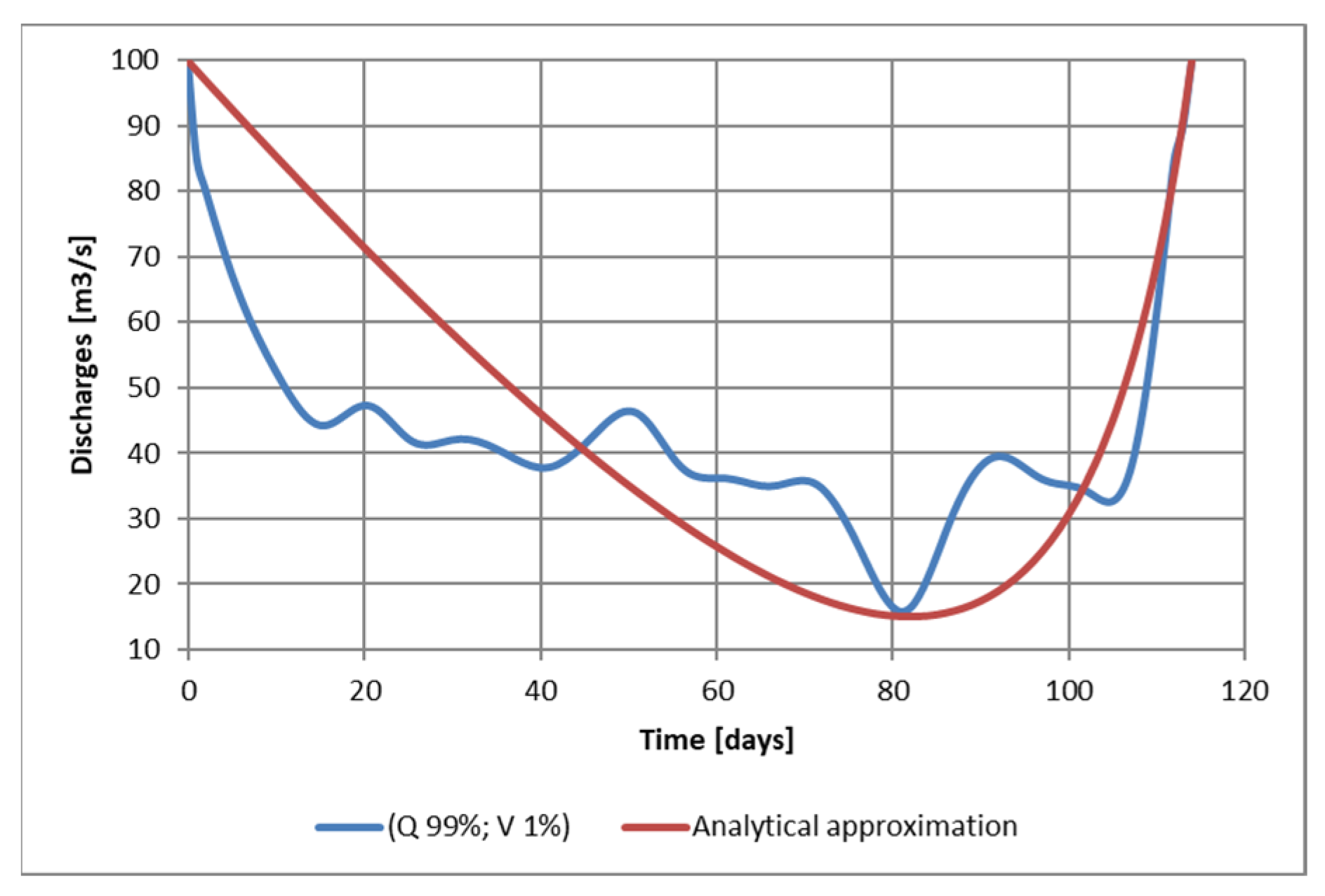
6. SDHs that reproduce the shape of registered droughts are more plausible than analytically defined SDHs. A polynomial interpolation was used to define the analytical approximation of the SDH. According to the interpolation theorem, there exists a unique polynomial of degree 2 that interpolates 3 data points. The coefficients of the polynomial were obtained considering a DH passing through the characteristic points (Figure 1): and preserving the deficit volume (Figure 13). Additionally, different skewed statistical distributions could be adjusted.
7. The same methodological approach can be used to derive SDHs for aquifers. However, water levels in observation wells will be analyzed instead of drought discharges. Based on these and a regional approach, SDHs can be derived for the entire aquifer upstream of the main abstraction works.
5. Conclusions
Assessment of SDH is extremely important for the management of available water resources in rivers, reservoirs and aquifers
The presented approach was used for local analysis of hydrological drought. However, this analysis can be made for all gaging stations in a river basin, obtaining the drought hydrological parameters at the river basin level [11]. To correct any anomalies and reconcile the local parameters with the same upstream and downstream parameters of the current location, a spatial analysis along the river network is needed. SDH at a particular gaging station integrates the upstream drought situation and provide information to water managers about available water resources. The hydrological processing of drought discharges can be performed to varying degrees of complexity. The simplest way is to consider the minimum discharge corresponding to a probability of exceedance P%. This value is necessary for establishing the ecological flow as well the security degree of the water levels at the water intakes. However, the deficit volume is also important in deciding the best allocation rules of existing water resources. This means that both minimum discharges and deficit volumes must be considered together. If they are correlated variables, the use of copulas is indicated to characterize the pairs of values (minimum discharge, deficit volume). If they are not correlated or the correlation is weak, each of the two variables may be analyzed individually for their statistical characterization. The minimum drought discharge is associated with high exceedance probability values. On the contrary, high deficit volumes are of interest, which means that they should be associated with low values of exceedance probabilities.
Different distributions can be used to fit the registered values of the minimum discharges and deficit volumes. All distributions approximate well the frequent values of the drought parameters, but they differ in the low-probability domain. Statistical tests followed by plotting the distributions that best fit the partial time series led to the choice of the most adequate distributions.
A challenging task, following the statistical characterization, is the choice of the pair that characterizes the probability of exceedance of minimum discharge and deficit volume. For illustrative purposes, the probabilities and have been considered complementary. However, other pairs of probabilities should be analysed to obtain a more complex assessment of drought scenarios.
In addition to minimum discharge and deficit volume, the shape of the drought hydrograph and total duration are also important. For this purpose, the drought hydrographs were normalized, and the dimensionless hydrographs were grouped into classes of similar shape. Based on the dimensionless hydrographs, the SDHs corresponding to different shape classes are obtained. The most critical events will be used for defining the best drought management strategies using existing water resources in rivers, reservoirs, and aquifers.
Author Contributions
Conceptualization, R.D. and A.F.D.; methodology, R.D. and A.F.D.; software, A.F.D.; validation, R.D., N.S. and C.D.; formal analysis, N.S.; writing—original draft preparation, R.D.; writing—review and editing, A.F.D., N.S. and C.D.; visualization, C.D.; supervision, R.D. All authors have read and agreed to the published version of the manuscript.
Funding
The elaboration of this methodology was not financed by public funds.
Data Availability Statement
Data owner is the National Institute of Hydrology and Water Management (INHGA - Romania). Restrictions apply to the availability of these data according to the INHGA policy.
Acknowledgments
The authors are grateful to the anonymous reviewers for their helpful comments and suggestions.
Conflicts of Interest
The authors declare no conflict of interest.
References
- Gibbs, W.J. Drought—Its Definition, Delineation, and Effects; Special Environmental Report No.5; World Meteorological Organization: Geneva, Switzerland, 1975; pp. 1–40. ISBN 92-63-00403–X. [Google Scholar]
- Estrela, T.; Menéndez, M.; Dimas, M.; Marcuello, C.; Rees, G.; Cole, G.; Weber, K.; Grath, J.; Leonard, J.; Ovesen, N.B.; et al. Part 3: Extreme hydrological events: Floods and droughts. In Sustainable Water Use in Europe; Environmental issue report No 21; EEA: Copenhagen, Denmark, 2001; pp. 44–46. [Google Scholar]
- Wilhite, D.A.; Glantz, M.H. Understanding: The drought phenomenon: The role of definitions. Water Int. 1985, 10, 111–120. [Google Scholar] [CrossRef] [Green Version]
- American Meteorological Society. Meteorological drought-policy statement. Bull. Am. Meteorol. Soc. 1997, 78, 847–849. [Google Scholar]
- Tallaksen, L.M.; Van Lanen, H.A.J. (Eds.) Hydrological Drought. Processes and Estimation Methods for Streamflow and Groundwater; Developments in Water Science; Elsevier Science B.V.: Amsterdam, The Netherlands, 2004; Volume 48, p. 579. [Google Scholar]
- UNISDR. Drought Risk Reduction Framework and Practices: Contributing to the Implementation of the Hyogo Framework for Action; United Nations Secretariat of the International Strategy for Disaster Reduction (UNISDR): Geneva, Switzerland, 2009; p. 213. [Google Scholar]
- Van Loon, A.F.; Van Lanen, H.A.J. A process-based typology of hydrological drought. Hydrol. Earth Syst. Sci. 2012, 16, 1915–1946. [Google Scholar] [CrossRef] [Green Version]
- Tsakiris, G.; Pangalou, D. Drought Characterisation in the Mediterranean. In Coping with Drought Risk in Agriculture and Water Supply Systems; Advances in Natural and Technological Hazards Research; Iglesias, A., Cancelliere, A., Wilhite, D.A., Garrote, L., Cubillo, F., Eds.; Springer: Dordrecht, The Netherlands, 2009; Volume 26. [Google Scholar] [CrossRef]
- Nalbantis, I.; Tsakiris, G. Assessment of hydrological drought revisited. Water Resour. Manag. 2009, 23, 881–897. [Google Scholar] [CrossRef]
- Tsakiris, G.; Nalbantis, I.; Vangelis, H.; Verbeiren, B.; Huysmans, M.; Tychon, B.; Jacquemin, I.; Canters, F.; Vanderhaegen, S.; Engelen, G.; et al. A system-based paradigm of drought analysis for operational management. Water Resour. Manag. 2013, 27, 5281–5297. [Google Scholar] [CrossRef]
- Caillouet, L.; Vidal, J.-P.; Sauquet, E.; Devers, A.; Benjamin Graff, B. Ensemble reconstruction of spatio-temporal extreme low-flow events in France since 1871. Hydrol. Earth Syst. Sci. 2016, Discuss. [Google Scholar] [CrossRef] [Green Version]
- Laaha, G.; Gauster, T.; Tallaksen, L.M.; Vidal, J.-P.; Stahl, K.; Prudhomme, C.; Heudorfer, B.; Vlnas, R.; Ionita, M.; Van Lanen, H.A.J.; et al. The European 2015 drought from a hydrological perspective. Hydrol. Earth Syst. Sci. 2016, Discussions. [Google Scholar] [CrossRef] [Green Version]
- Sharma, T.C. A drought frequency formula. Hydrol. Sci. J. 1997, 42, 803–814. [Google Scholar] [CrossRef]
- Razmkhah, H. Comparing Threshold Level Methods in Development of Stream Flow Drought Severity-Duration-Frequency Curves. Water Resour. Manag. 2017, 31, 4045–4061. [Google Scholar] [CrossRef]
- Hisdal, H.; Stahl, K.; Tallaksen, L.M.; Siegfried Demuth, S. Have streamflow droughts in Europe become more severe or frequent? Int. J. Climatol. 2001, 21, 317–333. [Google Scholar] [CrossRef]
- Stedinger, J.R.; Vogel, R.M.; Foufoula-Georgiou, E. Frequency Analysis of Extreme Events. In Handbook of Hydrology; Maidment, D.R., Ed.; McGraw-Hill: New York, NY, USA, 1993; pp. 18.1–18.66. [Google Scholar]
- Leadbetter, M.R. On a basis for ‘Peaks over Threshold’ modeling. Stat. Probab. Lett. 1991, 12, 357–362. [Google Scholar] [CrossRef]
- Bhunya, P.K.; Singh, R.D.; Berndtsson, R.; Panda, S.N. Flood analysis using generalized logistic models in partial duration series. J. Hydrol. 2012, 420–421, 59–71. [Google Scholar] [CrossRef]
- Ouarda, T.B.M.J.; Cunderlik, J.M.; St-Hilaire, A.; Barbet, M.; Bruneau, P.; Bobée, B. Data-based comparison of seasonality-based regional flood frequency methods. J. Hydrol. 2006, 330, 329–339. [Google Scholar] [CrossRef]
- Dracup, J.A.; Lee, K.S.; Paulson, E.G., Jr. On the definition of droughts. Water Resour. Res. 1980, 16, 297–302. [Google Scholar] [CrossRef]
- Tallaksen, L.M.; Madsen, H.; Bente Clausen, B. On the definition and modelling of streamflow drought duration and deficit volume. Hydrol. Sci. J. 1997, 42, 15–33. [Google Scholar] [CrossRef]
- Corzo Perez, G.A.; Van Huijgevoort, M.H.J.; Voß, F.; Van Lanen, H.A.J. On the spatio-temporal analysis of hydrological droughts from global hydrological models. Hydrol. Earth Syst. Sci. 2011, 15, 2963–2978. [Google Scholar] [CrossRef] [Green Version]
- Favre, A.C.; El Adlouni, S.; Perreault, L.; Thiémonge, N.; Bobée, B. Multivariate hydrological frequency analysis using copulas. Water Resour. Res. 2004, 40, W01101. [Google Scholar] [CrossRef] [Green Version]
- Salvadori, G.; De Michele, C. Frequency analysis via copulas: Theoretical aspects and applications to hydrological events. Water Resour. Res. 2004, 40, W12511. [Google Scholar] [CrossRef]
- Kitte, G.W. Frequency and Risk Analysis in Hydrology, 4th ed.; Water Resources Publications: Fort Collins, CO, USA, 1988; pp. 4–26. [Google Scholar]
- Drobot, R.; Draghia, A.F.; Ciuiu, D.; Trandafir, R. Design Floods Considering the Epistemic Uncertainty. Water 2021, 13, 1601. [Google Scholar] [CrossRef]
- Shanin, M.; Van Oorschoft, H.J.L.; De Lange, S.J. Statistical Analysis in Water Resources Engineering; Balkema: Rotterdam, The Netherlands, 1993; p. 241. [Google Scholar]
- Maidment, D.R. Handbook of Hydrology. Ch. 18. In Frequency Analysis of Extreme Events; McGraw-Hill: New York, NY, USA, 1993; pp. 18–54. [Google Scholar]
- Hingray, B.; Picouet, C.; Musy, A. Hydrologie. Une Science Pour l’ingénieur; Presses Polytechniques et Universitaires Romandes: Lausanne, Switzerland, 2014; p. 349. [Google Scholar]
- Wang, M.; Jiang, S.; Ren, L.; Xu, C.-Y.; Shi, P.; Yuan, S.; Liu, Y.; Fang, X. Nonstationary flood and low flow frequency analysis in the upper reaches of Huaihe River Basin, China, using climatic variables and reservoir index as covariates. J. Hydrology. 2022, 612 Pt C, 128266. [Google Scholar] [CrossRef]
- Ang, A.H.-S.; Tang, W.H. Probability Concepts in Engineering, Emphasis on Application to Civil and Environmental Engineering, 2nd ed.; John Wiley & Sons: San Francisco, CA, USA, 2006; p. 432. [Google Scholar]
- Koutsoyiannis, D. Uncertainty, entropy, scaling, and hydrological statistics. Hydrol. Sci. J. 2005, 50, 381–404. [Google Scholar]
- Chow, V.T.; Maidment, D.; Mays, L. Applied Hydrology; McGraw-Hill: Singapore, 1988; pp. 394–395. [Google Scholar]
- Chen, M.; Papadakis, K.; Jun, C. An investigation on the non-stationarity of flood frequency across the UK. J. Hydrol. 2021, 597, 126309. [Google Scholar] [CrossRef]
- Pettit, A.N. A non-parametric approach to the changepoint problem. Appl. Stat. 1979, 28, 126–135. [Google Scholar] [CrossRef]
Figure 1.
Hydrological drought parameters.

Figure 2.
Examples of drought shapes: (a) shape 1; (b) shape 2; (c) shape 3.

Figure 3.
Occurrence and duration of drought episodes.

Figure 4.
Correlations: (a) drought duration-deficit volume and (b) minimum discharge-deficit volume.
Figure 4.
Correlations: (a) drought duration-deficit volume and (b) minimum discharge-deficit volume.

Figure 5.
Drought hydrographs: (a) maximum deficit volume/duration and (b) minimum discharge.

Figure 6.
Minimum discharges at Lungoci gaging station (Siret River): (a) Wakeby distribution and (b) Johnson SB distribution.
Figure 6.
Minimum discharges at Lungoci gaging station (Siret River): (a) Wakeby distribution and (b) Johnson SB distribution.

Figure 7.
Deficit volumes at Lungoci gaging station (Siret River): (a) Pearson 6 distribution; (b) Johnson SB distribution.
Figure 7.
Deficit volumes at Lungoci gaging station (Siret River): (a) Pearson 6 distribution; (b) Johnson SB distribution.

Figure 8.
Shape of dimensionless droughts: (a) Class 1; (b) Class 2; (c) Class 3; (d) Class 4; (e) Class 5; (f) Class 6.
Figure 8.
Shape of dimensionless droughts: (a) Class 1; (b) Class 2; (c) Class 3; (d) Class 4; (e) Class 5; (f) Class 6.

Figure 9.
Synthetic drought hydrographs (Johnson SB distribution):(a1–a3) ; (b1–b3) ; (c1–c3) ; (d1–d3) .
Figure 9.
Synthetic drought hydrographs (Johnson SB distribution):(a1–a3) ; (b1–b3) ; (c1–c3) ; (d1–d3) .


Figure 10.
Synthetic drought hydrograph—Class 3.

Figure 11.
Synthetic drought hydrographs for classes 3, 4 and 6.

Figure 12.
Synthetic drought hydrographs Class 3: ; ; .

Figure 13.
Synthetic drought hydrograph and its analytical approximation.


Table 1.
Minimum drought discharges at Lungoci gaging station (m3/s).
| Exceedance Probabilities | 50% | 80% | 90% | 95% | 99% | 99.9% |
|---|---|---|---|---|---|---|
| Wakeby | 29.5 | 23.7 | 20.2 | 18.0 | 15.9 | 15.4 |
| Johnson SB | 29.4 | 23.8 | 20.6 | 18.4 | 15.5 | 14 |
Table 2.
Deficit volumes at Lungoci gaging station (mil. m3).
| Exceedance Probabilities | 0.1% | 1% | 5% | 10% | 20% | 50% |
|---|---|---|---|---|---|---|
Pearson 6 | 6386 | 1224 | 374 | 219 | 124 | 50 |
Johnson SB | 637 | 567 | 402 | 285 | 161 | 46 |
Table 3.
SDHs parameters (Johnson SB distribution).
Johnson SB (m3/s) | Johnson SB (mil. m3) | |||||
|---|---|---|---|---|---|---|
| 15.5 | 567 | 116 | 112 | 103 | ||
| 18.4 | 402 | 84 | 81 | 75 | ||
| 20.6 | 285 | 62 | 60 | 56 | ||
| 23.8 | 161 | 36 | 35 | 32 |
Table 4.
SDHs parameters for Johnson SB and Pearson 6 distributions.
Johnson SB (m3/s) | Pearson 6 (mil. m3) | |||||
|---|---|---|---|---|---|---|
| 15.5 | 1224 | 251 | 242 | 225 | ||
| 18.4 | 374 | 79 | 76 | 70 | ||
| 20.6 | 219 | 47 | 45 | 42 | ||
| 23.8 | 124 | 28 | 27 | 25 |
Disclaimer/Publisher’s Note: The statements, opinions and data contained in all publications are solely those of the individual author(s) and contributor(s) and not of MDPI and/or the editor(s). MDPI and/or the editor(s) disclaim responsibility for any injury to people or property resulting from any ideas, methods, instructions or products referred to in the content. |
© 2022 by the authors. Licensee MDPI, Basel, Switzerland. This article is an open access article distributed under the terms and conditions of the Creative Commons Attribution (CC BY) license (https://creativecommons.org/licenses/by/4.0/).
Share and Cite
MDPI and ACS Style
Drobot, R.; Draghia, A.F.; Sîrbu, N.; Dinu, C. Synthetic Drought Hydrograph. Hydrology 2023, 10, 10. https://doi.org/10.3390/hydrology10010010
AMA Style
Drobot R, Draghia AF, Sîrbu N, Dinu C. Synthetic Drought Hydrograph. Hydrology. 2023; 10(1):10. https://doi.org/10.3390/hydrology10010010
Chicago/Turabian StyleDrobot, Radu, Aurelian Florentin Draghia, Nicolai Sîrbu, and Cristian Dinu. 2023. "Synthetic Drought Hydrograph" Hydrology 10, no. 1: 10. https://doi.org/10.3390/hydrology10010010
Note that from the first issue of 2016, this journal uses article numbers instead of page numbers. See further details here.