Article

Achieving Real-World Saturated Hydraulic Conductivity: Practical and Theoretical Findings from Using an Exponential One-Phase Decay Model

1
Institut International d’Ingénierie de l’Eau et de l’Environnement (2iE), Ouagadougou 01 01 BP 594, Burkina Faso
2
IHE Delft Institute for Water Education, Westvest 7, 2611 AX Delft, The Netherlands
3
Independent Researcher, 1 rue Croix Saint Etienne, 58180 Marzy, France
*
Author to whom correspondence should be addressed.
Hydrology 2023, 10(12), 235; https://doi.org/10.3390/hydrology10120235
Submission received: 8 October 2023 / Revised: 16 November 2023 / Accepted: 20 November 2023 / Published: 9 December 2023
(This article belongs to the Section Hydrological and Hydrodynamic Processes and Modelling)

Abstract

:
Obtaining accurate values of saturated hydraulic conductivity (Ksat) is very important for managing all natural or artificial processes involving water flow into soils. Double-ring infiltration (DRI) is one of the easiest-to-work-with techniques commonly used for Ksat determination. Unfortunately, when improperly used, it leads to important variations and inaccurate results. This study was designed to investigate the necessary conditions to reach the true-value or real-world saturated hydraulic conductivity (Ksat-real-world) in the field. For this purpose, the effects of two factors—namely, the measured infiltration data type (cumulative, instant rate, and average rate) and the related non-linear regression equation type—were analyzed. Measurements with DRI were performed with samples from 106 locations in three West African countries, namely, Burkina Faso, Mali, and Cote d’Ivoire. The soils were composed of loam, sandy loam, and sandy clay loam. The results show that when infiltration rates are used rather than cumulative infiltration non-linear regression curves, the variability between the measured Ksat and the real-world saturated hydraulic conductivity (Ksat-real-world) could reach from 2.2% to 58.8%. This variability was caused by the approximate amplification—according to the procedure used—of time-increment measurement errors. Extending the test duration to more than 4 h, especially when clay soils were involved, and using the exponential one-phase decay non-linear regression of the cumulative infiltration data based on a clear measurement protocol provided the Ksat values that were closest to Ksat-real-world.

1. Introduction

Saturated hydraulic conductivity (Ksat) stands out as one of the most important characteristics of soil, and its accurate determination is essential to the success of in-soil crop-growing projects. The saturated hydraulic conductivity has an impact on both the ante- and post-development stages of soil [1]. For example, the choice of irrigation system type—e.g., surface irrigation, sprinkler irrigation, or localized irrigation—and the associated cropping pattern (rice, maize, vegetables) suitable for certain soils have to be preceded by measurement campaigns to map Ksat values, which will help with decision making. However, the pre-existence of certain types of vegetation or crop also induces changes and impacts on the Ksat by changing the soil structure, as observed when a forest is replaced with an agricultural area [2].
The top soil pounding infiltration technique has been extensively used for a long time to determine agricultural and even urban soil properties. In history, the principle of this technique has evolved into two types of equipment. The first was proposed to be a “single ring” (SRI) and is considered by some studies to be as accurate as the second and more common configuration, named “double ring” (DRI), as far as the determination of saturated hydraulic conductivity (Ksat) is concerned [3,4]. The usefulness of the technique is now admitted. DRI has been used, for example, to evaluate the difference in infiltration that would result from the decision to apply organic matter in soils [5]. In the Sudan savanna, Ikazaki et al. [6] found, by using DRI, that minimum tillage (MT, a minimum soil disturbance and soil cover technique) and sorghum residue mulching (a minimum soil disturbance technique) without intercropping effectively reduced the annual soil loss by 54%. The study was designed to assess the differential importance of each of the three components of conservative agriculture, defined by the Food and Agriculture Organization of the United Nations (FAO) as being (i) minimum soil disturbance, (ii) soil cover, and (iii) crop rotation/association. This result was explained by an improvement in the soil hydraulic conductivity through the boring of termites and wolf spiders found under the sorghum stover mulch. Aiming to assess the effects of agricultural wastes on the hydraulic properties of loamy sand cropland in Turkey, Gülser and Candemir [7] used DRI and found that a high carbon/nitrogen ratio in agricultural waste leads to a significant increase in the initial infiltration rate of loamy sand soil. Exploring the impact of irrigation water’s chemical composition on saline–sodic and normal soils, a study implemented both in the laboratory and on fields in India using DRI concluded that saturated hydraulic conductivity could drastically change in soils with a light texture as they were irrigated by chemical water [8]. None of these studies targeted the accuracy of DRI.
Other investigations examined the factors that may have an impact on the measurements carried out via DRI. Such factors included the diameter of the inner ring; the depth at which both rings are driven into the soil; the single-ring and double-ring comparative effect; the temperature; the water viscosity; and the time of measurement. In China, in an in situ study using different double-ring infiltrator diameters—20 cm, 40 cm, 80 cm, and 120 cm—and in three types of texture (loamy sand, silt, and silt loam) covering seven measurement sites, through performing numerical simulations using the software HYDRUS-2D model (Version 2.0), Lai and Ren [9] found that the size of the inner ring during DRI significantly alters the measured hydraulic conductivity of heterogeneous soil. The field test used a constant-water-level double-ring infiltrator. The results showed that the variability in the measured hydraulic conductivity was greater for smaller inner rings. The field tests reported that a steady flow state was reached within 90 min on average and that the criterion to terminate the test was that the volume infiltrated in 5 min “remains constant for a 30 min period”. In another study performed through simulation using the HYDRUS-2D model, Lai and Ren [10] investigated how the depth at which the double-ring infiltrator is driven into the soil could impact the hydraulic conductivity measurements. The results showed that the inner ring depth had a greater impact on Ksat than the outer ring and that a depth of 5–15 cm, as is traditionally used in infiltration measurements, was acceptable, as further pushing down would result in soil and hydraulic conductivity disturbances. The duration of infiltration was 120 min in all the simulations.
Several investigations were performed to compare the accuracy of the instant infiltration rate when using a single-ring infiltrometer (SRI) or a double-ring infiltrator. Wu et al. [11] used simulations based on numerically solving the axisymmetric form of the Richard equation. They considered one-dimensional infiltration as the referential value and compared this with results obtained with an SRI (diameter: 20 cm), a double-ring infiltrator (inner ring: 30 cm; outer ring: 30 cm), and other diameters. The purpose of the study was not specifically to obtain the value of saturated hydraulic conductivity (Ksat). The simulations yielded variations in the relative infiltration rate—expressed as the ratio of instant infiltration over Ksat (i/Ksat)—as a function of time. The values of Ksat were read from the literature for the three types of soils used in the simulations. Among other things, the study concluded that the DRI rates were about 80% of the one-dimensional infiltration vertical infiltration rates, while the infiltration rates of the SRI were f times greater than the one-dimensional infiltration rates, with f being a correction factor dependent on soil initial boundary conditions and ring geometry. Lewis et al. [3] conducted a study to compare the results of a single-ring infiltrometer (SRI) and a DRI. The measurements were performed on four sites in situ, with 4 replicates of 13 different experimental conditions or factor levels [12], which yielded 52 pairs of experimental units. The results showed that SRI and DRI lead to similar saturated hydraulic conductivity Ksat values for a wide range of soil conditions. The duration of the SRI tests was from 20 min to 90 min while DRI tests lasted from 30 min to 180 min. Interestingly, this study concluded that “the high variability of infiltration measurements by either method should be factored into study design when assessing infiltration rates”. Therefore, one should search for the variability causes through the measurement protocol and data-processing method.
Temperature and the daytime-measurement impacts on DRI measurements for saturated hydraulic conductivity were investigated by Clancy and Alba [13]. This study, implemented in the United States, rightly noted that the main issue with the in situ measurement of Ksat was its prominent variability. The study performed 67 Ksat measurements on sand and loamy sand soils across a temperature ranging from 5 °C to 35 °C. The references used for comparison were the values of Ksat, expressed as a function of water viscosity. The results showed that Ksat for sandy soils was from 2.0 to 2.9 times higher than the values predicted by the Ksat (viscosity) formula. The criterion for terminating the test was that the infiltration remained constant after three time increments of 5 min. The duration of the tests was, on average, 75 min. One of the main findings was that the time of day chosen to perform the tests affects the values. Morning measurements were found to be two times higher than the Ksat function of the viscosity, while afternoon measurements were nearly three times higher.
All the above investigations made substantial contributions to the use of the DRI technique to determine soil’s saturated hydraulic conductivity Ksat. Nevertheless, one cannot determine from the results whether the real-world Ksat-real-world was reached, for at least three reasons. Firstly, the duration of the tests was relatively short, generally not exceeding 90 min, while in cohesive soils, especially when clay is involved, it may take days and sometimes weeks to reach saturation. Secondly, none of the mentioned studies discussed the infiltration physical process pathway to select a suitable equation that would yield, after a confrontation with field measurement results, the Ksat-real-world. Finally, the measurement protocol (in terms of data collection and processing methods), although recognized to impact the reliability of the results, changes from author to author, and thus may hinder efforts to reach Ksat-real-world. The current study, implemented in three West African countries and covering 106 measurement sites, was designed to contribute to filling these gaps. In short, the aim of this study was to build a methodology based on theory and practice in order to obtain the true in situ saturated hydraulic conductivity Ksat-real-world.

2. Materials and Methods

2.1. Investigation Sites

Aiming to ensure potential usefulness for subsequent broader regional rural development activity, the sites of this study were selected for an accurate determination of their saturated hydraulic conductivity Ksat based on three main criteria. These criteria were: (i) a regional scope, with at least three countries whose economy is tightly linked to agriculture, (ii) the availability of different soils within or between the sites, and (iii) the existence of an irrigation project.
The three countries were Burkina Faso, Mali, and Cote d’Ivoire (Figure 1). Burkina Faso is a landlocked country in West Africa with an area of 274,200 km2. Its economy is largely based on agriculture, which employs 80% of the workforce [14]. Mali is also a landlocked country in West Africa, with an area of over 1,240,000 km2. The country has a traditional economic system in which the majority of the population engages in subsistence agriculture confined to the riverine area irrigated by the Niger River [15]. Cote d’Ivoire is a coastal country in West Africa, covering 322,463 km2. Cote d’Ivoire is heavily dependent on agriculture and related activities [16].
The soil types are related to the sites selected in each country (Table 1). The three sites of Burkina Faso—namely Kamboinsé, Goupana, and Rakaye—had, respectively, 2, 1 and 20 measurement points. These sites have soils that are essentially made of sandy loam, with occurrences of sandy clay loam and loam [17,18]. The three sites in Mali—namely BaguinedaUp, BaguinedaDwn, and Moria—received 61 measurement points. Their soils are mainly composed of sandy clay loam, with occurrences of loam and sandy clay. Finally, Sema was the unique site selected in Cote d’Ivoire, with 22 measurement points, covering soil made of sandy clay loam, with occurrences of loam.
The sites were either in use or destined for agricultural irrigation. The three sites of Burkina Faso were in use for localized irrigation, microsprinkler irrigation (Kamboinsé), and gravity irrigation (Goupana and Rakaye). In Mali, gravity irrigation was also either practiced (BaguinedaUp and BaguinedaDwn) [19] or planned for implementation (Moria). Gravity irrigation was planned for implementation in the Sema site in Cote d’Ivoire.

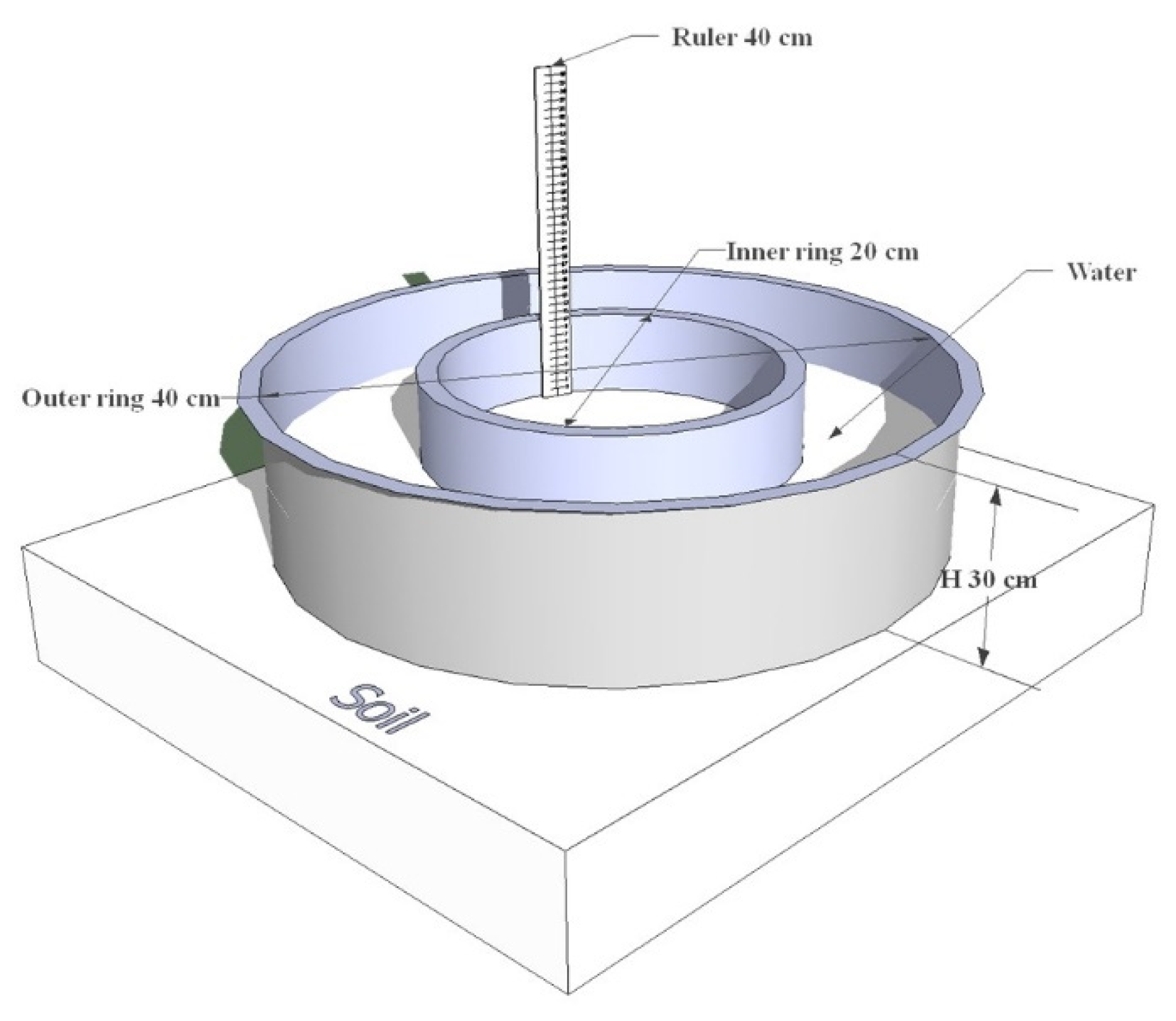
2.2. Double-Ring Infiltrometer

The double-ring infiltrometer is a well-known device to determine the soil infiltration curve and the saturated hydraulic conductivity. It has been used for various purposes related to saturated hydraulic conductivity, such as the determination of soil matrix infiltration in forest soils [20], simulations aiming to predict soil hydraulic parameters [21], or in comparing various infiltration devices’ biases [22]. Although sometimes automated and expensive [23], the basic device is essentially made of an inner ring and an outer ring (Figure 2). For the current investigations, the material was made of an inner ring with a diameter of 20 cm on the PVC pipe segment, and an outer ring with a diameter of 40 cm, also in the PVC pipe segment, with both having a height of 30 cm (Figure 2). However, as shown by Boivin [24], the size of the equipment—if not too small—has very little impact on the measurements. Before starting the measurement, the sites must be selected, and the number of sites will depend on the study area’s size. At least 9 measurement sites are required to study the soil parameters of 1.0 ha agricultural land. In this investigation, this figure was applied. Some 24 h before the real measurements started on a specific site, the soil was wetted by slowly pouring several bucket contents of water on the soil in order to raise the moisture toward saturation, thus reducing the testing time before saturation was reached. The wetting had another purpose: the inner and outer rings were pushed 5 cm into the soil using a plastic head hammer. This ensured that water would not circulate from the inner ring toward the outer ring, and from the outer ring to the surrounding soil surface; therefore, vertical flow would not occur at the soil surface. Afterward, a 40 cm height ruler was fastened to the wall of the inner ring so that water-level measurements could be carried out at the same location (Figure 2). The operator also used a stopwatch.
After the installation of the device, the measurements were performed according to a precise procedure. The procedure was as follows: (i) both the inner and the outer rings were filled with water to the edge; (ii) the stopwatch was started by the operator for a chosen measurement time increment. Based on pretests in the field, the time increments were generally set at 10 min for the first 3 measurements, 20 min for the following 3 measurements, 30 min for the third 3 measurements, and so forth. However, depending on how fast or slow the infiltration was occurring, the number of measurements at each time increment could be increased or reduced. After the preset time increment was reached, the stopwatch was stopped, and both the time increment ∆tmi and the related infiltrated water layer ∆hmi were measured (read) by the operator. Then, the water level in both rings was refilled to the edges, and the chronometer was initialized and run again. After a preset time increment elapsed, a new measurement of the quantities (∆hmi, ∆tmi) was performed. In this study, the operator knew that the saturation zone was reached by calculating the infiltration rate ∆hmi/∆tmi of the measured water layer increment ∆hmi and the related measured time increment ∆tmi, and by noticing that this rate no longer changed for three consecutive measurements. The constancy of the rate denoted that the soil moisture had reached the saturation zone from which the saturated hydraulic conductivity Ksat could be drawn.

2.3. Measured Variables

Among the field measurement data, three variables are particularly important because they are used to make a comparison between the expressions modeling the infiltration process and to determine the saturated infiltration rate Ksat of the soil. These three variables are the measured cumulative infiltration ht,cum-,meas (mm) (see Equation (2)), the measured instant infiltration rate iinst-meas (mm h−1) (see Equation (3)), and the measured average infiltration rate iavrg-meas (mm h−1) (see Equation (4)). Before these variables were determined, the primary data measured in the field were the infiltrated water layers and their related time values, as expressed in Equation (1):
Δ h t , m e a s =   h t , m e a s h t 1 , m e a s ,
where  Δ h t , m e a s (mm) is the incremental water layer, computed as the difference between the water level  h t , m e a s (mm) measured at time t and the water level  h t 1 , m e a s (mm) measured at time t−1. The index “meas” is related to the measured data.
The measured cumulative infiltration is expressed by:
h t , c u m m e a s =   h t 1 , c u m m e a s + Δ h t , m e a s ,
where  h t , c u m m e a s (mm) is the cumulative water layer infiltrated from the beginning of the test to the instant current time t. This time t is actually the sum (so a cumulation) of individual time increments  Δ t m e a s  corresponding to  Δ h t , m e a s , the incremental infiltrated water layer determined in Equation (1). The quantity  h t 1 , c u m m e a s  is the cumulative water layer infiltrated at the previous time t−1. The index “meas” is related to the measurement data.
The measured instant infiltration rate was given by:
i i n s t m e a s = Δ h t , m e a s Δ t   ,
where  i i n s t m e a s  is the instantaneous infiltration rate measured at instant t, expressed as the ratio of  Δ h t , m e a s  as determined in Equation (1), with the time increment Δt being the duration between the measurements of the water level  h t , m e a s (mm) and the water level  h t 1 , m e a s .
The measured average infiltration rate was provided by:
i a v r g m e a s = h t , c u m m e a s t ,
where  i a v r g m e a s (mm h−1) is the average infiltration rate measured, expressed as the ratio of the cumulative infiltrated water layer  h t , c u m m e a s (mm) determined in Equation (2) and the elapsed time t (h) (from the beginning of the test).
The couples of measured data—( h t , c u m m e a s , t ); ( i i n s t m e a s , t ); ( i a v r g m e a s , t )—would be plotted against their non-linear regression [12,25] counterparts (cf. Section 3.2) to determine which model will yield a Ksat result that is as close as possible to the real-world or true value.

2.4. Processed Variables

Similar to the measured variables, three processed variables are of special importance because they can be used to determine which among the measurement expressions and mathematical models would lead to the closest real-world saturated infiltration Ksat values. Conversely to the measurement, the first variable to be considered here is the instant infiltration rate because it better analytically models the infiltration process. The evolution of infiltrated water layer speed follows a process that is regularly found in nature [26]: a certain quantity varies at a speed that is proportional to the remaining amount of that quantity. In the case of soil infiltration measurement with a double ring, the infiltration speed depends on the standing water layer in the inner ring (Figure 2). Analytically, this relationship is expressed by Equation (5):
i t ( t ) = d h d t ,
where  i t ( t )  (mm h−1) is the instant infiltration rate;  d h (mm) and  d t (h) are, respectively, water-level variation and the related duration.
Many processes occurring in nature follow the pattern described in Equation (5). For example, the determination of soil infiltration rate, the decay of radioactive isotope atoms [27,28], and the turnover of blood cells in HiV-1 infection [29].
It can be shown that the exponential one-phase decay function is a solution of Equation (5). Therefore, the instant infiltration equation is rewritten, yielding the first processed variable:
i t ( t ) = d h d t = Regr   i i n s t m e a s = k s a t + ( i 0 k s a t ) e b t ,
where  t ( h )  is the elapsed time,  k s a t (mm h−1) is the saturated infiltration rate toward which the instant infiltration rate will tend as time increases;  i 0 (mm h−1) is the initial infiltration rate at the beginning of the tests;  b  is a coefficient of decay that can be determined through non-linear regression applied to the infiltration data collected from a double-ring test. In other words, the three parameters ( k s a t i 0  and  b ) of Equation (6) can be completely determined by running a non-linear regression on the field data ( Δ h t , m e a s , Δ t ) measured for Equation (3). The resulting equation is Regr inst-meas, in which numerical values are assigned to  k s a t i 0 , and  b .
The cumulative form is obtained from Equation (6) by the following analytical summation:
d h d t = k s a t + ( i 0 k s a t ) e b t d h = k s a t d t + ( i 0 k s a t ) e b t d t h 0 h c u m d h = t 0 t k s a t d t + t 0 t ( i 0 k s a t ) e b t d t .
This computation yields the second processed variable:
h c u m = Regr   h c u m m e a s = k s a t t + 1 b ( i 0 k s a t ) ( 1 e b t ) ,
where the three parameters ( k s a t i 0  and  b ) of Equation (6) can be completely determined by running a non-linear regression on the field data ( h t , c u m m e a s , t ), measured for Equation (2).
Two things are worth noting when considering Equations (6) and (8). The first is that ksat, drawn from Equations (6) and (8), is exactly the same variable, since one equation is derived from the other. Hence, the values of ksat drawn from field data by either method (instant infiltration or cumulative infiltration) should be exactly the same, theoretically. Discrepancies observed between both would mean that errors occurred and must be elucidated. A second aspect that is worthy of notice is that both non-linear equations include a linear part in their curve: (i) for Equation (6), this linear portion is a horizontal line whose value is equal to ksat, while (ii) for Equation (8), this linear portion is an oblique line whose slope is equal to the same saturated hydraulic conductivity ksat. Therefore, being able to identify the moment when the linear portion of each of the curves—materialized by a straight line—appears will be crucial in the determination of the appropriate time to stop the measurements because ksat is reached.
The third processed variable is the average infiltration rate, obtained by running a non-linear regression analysis on the average data iavrg-meas determined in Equation (4), as follows:
Regr   i a v r g m e a s = k s a t + ( i 0 k s a t ) e b t ,
It is worth noting that the three parameters ( k s a t i 0  and  b ) obtained from the three regressions Equations (6), (8), and (9) are not necessarily expected to be the same. This point was analyzed by plotting the following variables alongside the remaining data: ( Regr   i i n s t m e a s , t ), ( Regr   h c u m m e a s , t ), and ( Regr   i a v r g m e a s , t ).

3. Results and Discussion

3.1. How False Saturated Infiltration Values Are Measured with Various Soil Types

The sample presented in Figure 3 provides insights into several important aspects of the infiltration process. In graphs a–d in the three countries, namely Burkina Faso, Mali, and Cote d’Ivoire, the plots of the cumulative infiltration measured in the field (1) and the related fitted non-linear regression curve (2), the rate of infiltration measured in the field (4), and the related fitted non-linear regression curve (5) are presented. Even based only on visual inspection (the fit parameters are reported in Section 3.2), these figures show, in general, a good fit for the cumulative infiltration data (Figure 3a–d(2)), while the fits of the instant rate of infiltration indicate important gaps compared to the field data (5a–d). For all measurements related to the instant infiltration rate (Figure 3a–d(5)) in the three countries, discrepancies persistently occur at the beginning of the field measurements. This observation points to the volatility of the instant infiltration rate quantity Δht because of the higher soil water absorption rate at the beginning [30], causing errors in the measurement of Δh, but with a greater impact from errors related to the denominator Δt. This hectic start influences the measured values and the regression fits that are produced based on the instant infiltration rate. The Ksat values obtained from the two processes—the one from the non-linear regression of the cumulative infiltration and the one from the instant rate of infiltration, respectively—are not equal. The results yield for Kamb-1, 6.2 mm h−1 versus 11.1 mm h−1; for Moria-P01, 7.7 mm h−1 versus 4.2 mm h−1; for Moria-P07, 8.2 mm h−1 versus 12.4 mm h−1; and for Sema-P05-RCI, 1.8 mm h−1 versus 2.0 mm h−1. Although the Ksat value for cumulative infiltration cannot be ascertained to be the best assessment (rightness) (see Section 3.2) of the real-world Ksat-real-world [31], it appears more precise (accuracy) because of the systematic better goodness of fit.
The comparison between the average infiltration rate and the measured instant infiltration rate also reveals gaps, whose analysis leads to important clarifications. The two processes are illustrated in Figure 4. Three observations can be made. First, the instant infiltration rate data (Figure 4a–d(4)) tend to be systematically smaller than the average infiltration rate data (Figure 4a–d(6)). Therefore, one would expect a lower saturated hydraulic conductivity Ksat from the instant infiltration rate measurements. It could be that the average infiltration equation (Equation (4)) denominator, deduced from measurements from the beginning of the test to a certain elapsed time t (the sum of the incremental Δt) is marked by errors that tend to minimize the real duration related to the absorption of the water height hcum-meas. This involuntary shortening of the duration would lead to higher average infiltration rates. In fact, the same type of error occurs in incremental Δt measurements related to the instant infiltration rate in Equation (3), but its magnitude is much smaller than the one related to measurements of the average infiltration rate after 3 h or 5 h. The second observation from the processes depicted in Figure 4 is that, from graphical inspection, it can be seen that the goodness of fit of both infiltration processes is rather bad, at least until the midpoint of the test. The midpoints of the presented sample are 25 h for Kamb-1, 9 h for Moria P01, 5.5 h for Moria P07, and 4 h for Sema P05. It is only near the end of the process that the fit is good. This observation supports the assumption that the saturated hydraulic conductivity is better measured and modeled by non-linear regression when the soil moisture tends toward saturation [26,32]. The third and final observation is related to the fact that, as one would expect, instant infiltration rate data with shorter intervals of measurement are much more hectic than the average infiltration rate data. Hence, one would be prone to conclude that the latter would yield a more accurate Ksat than the former [33]. However, for the reasons provided in the previous observation, that is not the case (see further in Section 3.2). The Ksat values yielded by the average versus instant infiltration rates for the four sample sites are, respectively, 12.2 mm h−1 versus 11.1 mm h−1 for Kamb-1; 24.2 mm h−1 versus 14.2 mm h−1 for Moria-P01; 18.7 mm h−1 versus 12.4 mm h−1 for Moria-P01; and 6.3 mm h−1 versus 2.0 mm h−1 for Sema-P05. Finally, as explained in the comments relating to Figure 3, the instant infiltration rate does not lead to the real-world Ksat-real-world value.
With 2.5% organic matter content, Saxton [34] made the following classification of soils on the texture triangle: loam for Ksat from 8.6 to 46.9 mm/h; clay loam for Ksat from 2.01 to 7.79 mm/h; and sandy clay loam for Ksat between 3.94 and 20.06 mm/h. It can be noted that these three types of soil have overlapping areas in terms of Ksat, and for each type of soil, a whole range of Ksat exists. For example, the 6.2 mm h−1 of the site Kamb-1 is compatible with a loam, a clay loam, or even a sandy clay loam. Only a grain size analysis [35] will allow for a precise classification of the soils, though this does not hinder the importance of obtaining a real-world Ksat that could be used, for example, to design sprinkler irrigation systems [36].

3.2. What Field Investigations Reveal about Saturated Hydraulic Conductivity

3.2.1. Tracking the Real-World Ksat Value

The graphs displayed in Figure 5 are related to data samples collected and processed from 12 different testing sites out of the 106 addressed by this investigation. As shown in Table 1, many of the 106 investigation sites were located on similar soils. In each of the 12 graphs, the data are displayed, with identifying numbers and graph markers provided in the legend at the bottom of the graph. These numbers are as follows: “1” for the cumulative infiltrated water layer—Equation (2); “4” for the measured instant infiltration rate—Equation (3); and “6” for the measured average infiltration rate—Equation (4). Based on these three series of data, a non-linear regression computation—Equations (6), (8), and (9)—was performed, and the results are presented in three other graphs, connected with lines. These graphs are identified by the following numbers: “2” for the non-linear regression related to the measured cumulative infiltration hcum-meas, “5” for the non-linear regression performed on the instant infiltration rate data, and “7” for the non-linear regression run on the average infiltration rate data. To show the mathematical expressions of the 36 regression curves in Figure 5, 12 exponential one-phase decay regression equations [32] are presented in Table 2. In this table, only one infiltration test site was selected from each country.
As can be clearly seen from the asymptotic lines of the non-linear regression curves shown in Figure 5 and the sample extracts in Table 2, for the same infiltration measurement site, the saturated hydraulic conductivity Ksat is different for the three regression processes, and sometimes the difference is rather significant. Based on Table 2, for example, Ksat is 6.2 mm h−1 at Kamb-1-Burkina Faso if cumulative infiltration measurement data are used, while it would be, respectively, 11.10 mm h−1 and 12.21 mm h−1 if instant and average infiltration measurement data were used. The results for the site of BaguinedaUp-Mali are very close, even though the value obtained from the cumulative infiltration curve is the smallest. The results for this site yield a Ksat of 3.1 mm h−1 when cumulative infiltration measurement data are used, and 3.1 mm h−1 and 3.8. mm h−1, respectively, if instant and average infiltration measurement data are used. However, the difference becomes significant again for the site of Sema-P1-Cote d’Ivoire: 2.3 mm h−1 with cumulative infiltration data, and 12.4 mm h−1 and 8.0 mm h−1, respectively, when instant and average infiltration measurement data are used.

3.2.2. The Best Saturated Hydraulic Conductivity Results

Considering the graphs shown in Figure 5, two important questions need to be addressed to derive useful conclusions about the saturated hydraulic conductivity measurement process: (i) What can be considered real-world Ksat-real-world? (ii) Which of the three procedures—deriving Ksat from non-linear regressions of hcum-meas, iinst-meas, and iavrg-meas—is better in terms of reaching Ksat-real-world? In real field experiments, when the soil moisture is brought close to saturation before the double-ring infiltration test starts, the cumulative infiltration curve remains a straight line, as can be seen in Figure 5e. It was noticed that, under these conditions, the values of the three regression lines were generally close, as for BaguinedaUp-Mali. From the graphs in Figure 5, it can also be deduced that two factors are very important: (a) the measurement of time increments Δt (particularly in the curvature zone), and (b) the number of available data for the asymptote branch of the curve. When Δt is constant and Δh is constant, measurements are generally inaccurate and Ksat will not be valid. To follow the real-world process of infiltration, the operator must exponentially dilate either Δt or decrease Δh to capture the filling of the exponential decrease in infiltration. When the linear segment of the infiltration rate curves is reached, then the ratio Δht must remain constant, regardless of the values of Δh and Δt. Therefore, when the ratio (Δht)meas—computed directly from the measured data in the field—remains constant for three consecutive measurements, the soil saturation is reached and this constant value of (Δht)meas can be considered the real-world saturated hydraulic conductivity Ksat-real-world. Reaching this value can be time-consuming in practice, especially when dealing with clayey soils. This is why regression analysis is very relevant: its prediction allows for the determination of a Ksat that is as close as possible to Ksat-real-world.
In order to answer the question “Which of the three procedures—deriving Ksat from non-linear regressions of hcum-meas, iinst-meas, and iavrg-meas—is better in terms of reaching Ksat-real-world?”, comparative figures of Ksat are shown in Table 3. In the table, three quantities assessing the goodness of fit of non-linear regression are shown in columns 6–8. These are as follows: (i) R2, the coefficient of determination (the closer to 1, the better), (ii) SSE, the error sum of squares (the smaller, the better) [37], and (iii) MSE, the mean of squared error (the smaller, the better) [38]. In the ninth column, the values of the saturated hydraulic conductivity Ksat—derived from their respective non-linear equations—are shown for each of the 12 individual sites and each of the three procedures. In the 10th column that follows Ksat, the average of the last three measurements (Δht)meas is presented. These values, as explained in the previous paragraph, can be considered the real-world or true saturated hydraulic conductivity Ksat-real-world. The gap or discrepancy between Ksat and Ksat-real-world is shown in the last column of the table. For all 12 sites, it appears that the procedure that best estimates the saturated hydraulic conductivity is the one using the cumulative infiltration measurement data (Table 3(1–12a)). The gaps in absolute values vary from 2.2% to 58.8%. The worst estimation procedure is the averaging one, with a maximum gap reached on the site of Sema of 444.4%. The instant infiltration procedure is located between the two previous ones. Therefore, it can be stated that the cumulative infiltration measurement data procedure is the best way to estimate the saturated hydraulic conductivity of soil Ksat. Once that is stated, the question is: how is the cumulative infiltration procedure more accurate than the instant infiltration rate procedure? A discussion based on both analytical expressions and graphics will help in answering this question.

3.3. Searching for the Equation That Yields more Accurate Saturated Hydraulic Conductivity

It is helpful to use the cumulative infiltration curve as the basis to assess which of the two non-linear regressions, Equations (6) and (8), will yield the most accurate saturated hydraulic conductivity. In Figure 6, it can be seen that errors occur during both the water-height interval measurements Δhmi and the time interval measurements Δti. Therefore, each individual segment of the measurement curve can be computed using the Pythagorean theorem [39] for rectangular triangles, as shown in Equation (10):
Δ C i 2 = Δ h i 2 + Δ t i 2 ,
where ΔCi is the length of individual segments of the measurement curve; Δhi is the infiltrated water increment; and Δti is the time increment.
Time and water head are independent variables at the macroscopic scale, and, as such, can be measured simultaneously with an arbitrary accuracy [40]. However, in practice, water head measurement errors are much more easily minimized by a good operator and an accurate limnimetric device (Figure 2). Therefore, it is assumed that most errors only occur during the cumulative time interval measurements  Δ t m i . With these hypotheses, the positive error  ε c i  between each individual segment  Δ c k  of the measurement curve when plotted against the corresponding regression curve segment (Figure 6) can be calculated using Equation (11):
ε C i = ( ε t i 1 + ε t i ) ,
where  ε c i  is the error in absolute value (hence, positive) or the gap between each individual segment of the measurement curve and the (theoretically adjusted) non-linear regression curve, while  ε t 1 ε t 2 ε t 3 , are the curve segment errors induced by time errors during the measurements of time increments  Δ t m 1 Δ t m 2 Δ t m 3 , such as
t m i = t i + ε t i ,
where  t m i  is the cumulative measured time (“m” stands for measured);  t i  is the theoretical (true) cumulative time;  ε t i  is the time measurement error.
From the construction graph in Figure 6, the following can be derived:
ε t i = t i ( t m i 1 + Δ t m i ) ,
By inserting Equation (13) into Equation (11):
ε C i = ( t i + t i 1 ) ( t m i 1 + t m i 2 ) ( Δ t m i + Δ t m i 1 ) ,
The structure of Equation (14) shows two important aspects that can help to ensure more accurate infiltration measurements. First, as in any time series [41,42,43], the error  ε C i  at time step i depends on the errors in current measurements  t m i , but also on measurements at previous times steps  t m i 1  and  t m i 2 . As written by Montgomery [41], in time series, a future observation depends on the current and the past observations, i.e., adjacent observations are dependent. There is an autocorrelation in the data. Secondly, the second and the third terms on the right side of Equation (14) constitute the random part of the error [41], with the deterministic part being  t i + t i 1 , and show that the greater the interval between two measurements, the larger the gap between the real-world measurement and the regression curves. This result was expected since the straight line forming the curve segment ∆Ci will be longer and difficult to fit into a curved segment of the regression line. Therefore, ideally, to minimize the gaps between the two curves by altering  Δ t i , one would (i) proceed with independent measurements of time intervals by bringing the chronometer (and refilling the infiltrometer to reset the water head) to zero at each new measurement and (ii) choosing smaller time intervals. This last point, i.e., shortening the time interval, leads to two important proposals. The first is related to when it is better to keep short time intervals during the measurements. Field data (Figure 5) indicate that the change in the direction of the cumulative curve is faster at the beginning of the measurements and during the 4–5 following hours (depending on the soil type) than later on. This means that to keep the measurement curve as close as possible to the non-linear regression curve, one needs to use short time intervals  Δ t m i  at the beginning. However, while the soil becomes more and more saturated, the change in the direction of the cumulative regression curve slows down and the curve moves toward a straight line, with a constant slope, providing the expression of the saturated hydraulic conductivity:
K s a t = Δ h m s a t / Δ t m s a t ,
where  K s a t  is the saturated hydraulic conductivity;  Δ h m s a t  is the infiltrated water layer measured while the straight-line zone is reached; and  Δ t m s a t  is the time interval related to  Δ h m s a t .
Hence, when the soil gets closer to saturation [44], longer time intervals are suitable to ensure an accurate fitting between the measurement curve and the non-linear regression curves (Figure 6).
From the elements of analysis presented in Figure 6 and Equation (6), one can also see how drawing the saturated hydraulic conductivity from the instantaneous infiltration rate measurements would lead to inaccurate results. In effect, each point of the infiltration rate is obtained by the slope:
i m i = Δ h m i / Δ t m i ,
in which imi is the “measured” (in reality, “calculated”) instant infiltration rate;  Δ h m i i is, the measured infiltrated water layer; and  Δ t m i  is the time interval related to  Δ h m i .
The related error  ε i m i  is calculated (rather than measured) by applying the differential computation to Equation (16), which is a quotient, yielding:
ε i m i = ε h i Δ t m i Δ h m i ε t i Δ t m i 2 ,
As shown in the expression of Equation (17), the smaller the time interval of measurements  Δ t m i , which is suitable at the beginning of the infiltration measurements, as previously stated, the greater the error  ε i m i  in the soil infiltration rate data, resulting in important changes in the direction of the measurement curve. Due to these changes, the fitting between the infiltration rate measurement data and the related non-linear regression curve is generally worse than the discrepancies observed with the cumulative infiltration curves. As a result, the saturated infiltration value Ksat obtained from the measured data and the regression equation present important, irreducible gaps.
Therefore, even though authoritative standardization institutions such as ASTM [45] suggest deriving the permeability (saturated hydraulic conductivity) from infiltration rate data, this method usually leads to erroneous values. Hence, it is not surprising that, in its standard sheet D 5093-02 related to double-ring infiltration measurements, the values of Ksat for i are usually so scattered that ASTM did not provide any estimate of the errors.

3.4. A Protocol for Accurate In Situ Measurement of Soil Saturated Hydraulic Conductivity Ksat

When making infiltration measurements, it is always critical to determine when the investigation should be terminated [9,13]. As shown in Equation (15) and Figure 5, the saturated hydraulic conductivity Ksat is reached when the ratio of the hydraulic head variation and the related measured time interval becomes constant, or when the cumulative curve starts to change into a straight line. However, based on the experiments implemented in the three countries in this study, the figures indicate that when three consecutive computations of this ratio provide a constant, same value, the measurements could be stopped and Ksat can be derived from Equation (8). Therefore, a full procedure—considering the necessity of (i) having shorter time intervals at the beginning of the measurements and longer time intervals near the saturated zone, (ii) ending the trials at the right time when the infiltration process reaches saturation—is proposed in Table 4 and Table 5.
The way to proceed with the field operation is described in Table 4, while the data should be written as shown in Table 5. The time measurements are clustered into series from I to V (Table 5) allowing for a well-organized and accurate experiment. In each series, the time interval is constant. For example, in series I, this is 10 min, in series II, this is 20 min, in series III, this is 30 min, etc. In a real field experiment, only time intervals (3rd column) are measured and the values of the cumulative time T(h) in hours (4th column) are deduced from the intervals. In the 5th column, the infiltrated water head increments are measured and correspond to the time intervals of the 3rd column. The cumulative infiltrated water head values in the 6th column are computed from the values in the 5th column. Finally, only data from column 4 and column 6 are used to plot the measurement curve and compute, and, against those data, a non-linear regression curve is plotted using, for example, Minitab [46] or XLSTAT 2014.5.03 software [47].

4. Conclusions

Targeting accuracy in the measurement of saturated hydraulic conductivity Ksat, this study used data collected from 106 measurement locations in three West African countries. This showed how inaccurately Ksat is measured in many studies when (i) the test duration is too short, (ii) the infiltration rate and average infiltration rate data, rather than cumulative infiltration data, are used, (iii) non-linear regression equation of infiltration rates instead of cumulative infiltration data are used, and (iv) the criterion for the test termination is not clearly specified. The measurement duration varied in this study from 4 to 50 h, while most of the tests found in the literature would not last more than 3 h, not allowing for the infiltration rate to reach Ksat, especially when clay is involved. When infiltration rates are used instead of cumulative infiltration non-linear regression curves, the gap between the measured Ksat and the real-world saturated hydraulic conductivity Ksat-real-world was found to vary from 2.2% to 58.8%, even reaching 444.4% when average infiltration rate data were used. Using differential mathematical analysis, the study explained how operator errors in time measurement affect the infiltration rate more than cumulative infiltration curves and led to the conclusion that the cumulative infiltration measurement data procedure is the best way to estimate the saturated hydraulic conductivity of a soil Ksat. The study proposed a clear investigation protocol that would help to achieve real-world saturated hydraulic conductivity Ksat-real-world during investigations.

Author Contributions

Conceptualization, A.K., M.Z., M.D.F. and B.L.; formal analysis, A.K., M.Z. and B.L.; investigation, A.K. and B.L.; methodology, A.K., M.Z., M.D.F. and D.D.D.; writing—review and editing, A.K., M.Z. and Y.K.; visualization, A.K., M.Z. and D.D.D.; review and editing, A.K., L.G.H. and Y.K.; funding acquisition, D.D.D. and Y.K. All authors have read and agreed to the published version of the manuscript.

Funding

This work was financially supported by the World Bank through its Excellency Centre in Africa (CEA), a partner of the International Institute for Water and Environmental Engineering (2iE).

Data Availability Statement

The data presented in this study will be made available upon request.

Conflicts of Interest

The authors declare no conflict of interest.

References

  1. Zhu, P.; Zhang, G.; Zhang, B. Soil Saturated Hydraulic Conductivity of Typical Revegetated Plants on Steep Gully Slopes of Chinese Loess Plateau. Geoderma 2022, 412, 115717. [Google Scholar] [CrossRef]
  2. Hao, M.; Zhang, J.; Meng, M.; Chen, H.Y.H.; Guo, X.; Liu, S.; Ye, L. Impacts of Changes in Vegetation on Saturated Hydraulic Conductivity of Soil in Subtropical Forests. Sci. Rep. 2019, 9, 8372. [Google Scholar] [CrossRef] [PubMed]
  3. Lewis, J.; Amoozegar, A.; McLaughlin, R.A.; Heitman, J.L. Comparison of Cornell Sprinkle Infiltrometer and Double-Ring Infiltrometer Methods for Measuring Steady Infiltration Rate. Soil Sci. Soc. Am. J. 2021, 85, 1977–1984. [Google Scholar] [CrossRef]
  4. Reynolds, W.D.; Elrick, D.E. Ponded Infiltration From a Single Ring: I. Analysis of Steady Flow. Soil Sci. Soc. Am. J. 1990, 54, 1233–1241. [Google Scholar] [CrossRef]
  5. Fueki, N.; Lipiec, J.; Kuś, J.; Kotowska, U.; Nosalewicz, A. Difference in Infiltration and Macropore between Organic and Conventional Soil Management. Soil Sci. Plant Nutr. 2012, 58, 65–69. [Google Scholar] [CrossRef]
  6. Ikazaki, K.; Nagumo, F.; Simporé, S.; Barro, A. Are All Three Components of Conservation Agriculture Necessary for Soil Conservation in the Sudan Savanna? Soil Sci. Plant Nutr. 2018, 64, 230–237. [Google Scholar] [CrossRef]
  7. Gülser, C.; Candemir, F. Effects of Agricultural Wastes on the Hydraulic Properties of a Loamy Sand Cropland in Turkey. Soil Sci. Plant Nutr. 2015, 61, 384–391. [Google Scholar] [CrossRef]
  8. Singh, N.T.; Jaswal, S.S. Effect of Test Solution Composition on the Hydraulic Conductivity of Normal and Saline-Sodic Soils. Soil Sci. Plant Nutr. 1973, 19, 195–200. [Google Scholar] [CrossRef]
  9. Lai, J.; Ren, L. Assessing the Size Dependency of Measured Hydraulic Conductivity Using Double-Ring Infiltrometers and Numerical Simulation. Soil Sci. Soc. Am. J. 2007, 71, 1667–1675. [Google Scholar] [CrossRef]
  10. Lai, J.; Luo, Y.; Ren, L. Numerical Evaluation of Depth Effects of Double-Ring Infiltrometers on Soil Saturated Hydraulic Conductivity Measurements. Soil Sci. Soc. Am. J. 2012, 76, 867–875. [Google Scholar] [CrossRef]
  11. Wu, L.; Pan, L.; Roberson, M.J.; Shouse, P.J. Numerical Evaluation of Ring Infiltrometers under Various Soil Conditions. Soil Sci. 1997, 162, 771. [Google Scholar] [CrossRef]
  12. Montgomery, D.C. Design and Analysis of Experiments—Eigth Edition, 8th ed.; John Wiley & Sons: Phoenix, AZ, USA, 2013; ISBN 978-1-118-14692-7. [Google Scholar]
  13. Clancy, K.; Alba, V.M. Temperature and Time of Day Influence on Double-Ring Infiltrometer Steady-State Infiltration Rates. Soil Sci. Soc. Am. J. 2011, 75, 241–245. [Google Scholar] [CrossRef]
  14. Traore, O.; Wei, C.; Rehman, A. Investigating the Performance of Agricultural Sector on Well-Being: New Evidence from Burkina Faso. J. Saudi Soc. Agric. Sci. 2022, 21, 232–241. [Google Scholar] [CrossRef]
  15. Singbo, A.; Njuguna-Mungai, E.; Yila, J.O.; Sissoko, K.; Tabo, R. Examining the Gender Productivity Gap among Farm Households in Mali. J. Afr. Econ. 2021, 30, 251–284. [Google Scholar] [CrossRef]
  16. Golou Gizèle, Z.; Kouassi Bruno, K.; Yao Sadaiou Sabas, B.; Jan, B. Migration and Agricultural Practices in the Peripheral Areas of Côte d’Ivoire State-Owned Forests. Sustainability 2019, 11, 6378. [Google Scholar] [CrossRef]
  17. FAO; IUSS. World Reference Base for Soil Resources 2014: International Soil Classification System for Naming Soils and Creating Legends for Soil Maps—Update 2015; World Soil Resources Reports; FAO: Rome, Italy, 2015; ISBN 978-92-5-108369-7.
  18. Nachtergaele, F.; van Velthuizen, H.; Verest, L.; Wiberg, D. Harmonized World Soil Databaze—Version 1.2; FAO: Rome, Ital, 2012. [Google Scholar]
  19. Keïta, A.; Koïta, M.; Niang, D.; Lidon, B. WASO: An Innovative Device to Uncover Independent Converging Opinions of Irrigation System Farmers. Irrig. Drain. 2019, 68, 496–506. [Google Scholar] [CrossRef]
  20. Zhang, J.; Lei, T.; Qu, L.; Chen, P.; Gao, X.; Chen, C.; Yuan, L.; Zhang, M.; Su, G. Method to Measure Soil Matrix Infiltration in Forest Soil. J. Hydrol. 2017, 552, 241–248. [Google Scholar] [CrossRef]
  21. Mashayekhi, P.; Ghorbani-Dashtaki, S.; Mosaddeghi, M.R.; Shirani, H.; Nodoushan, A.R.M. Different Scenarios for Inverse Estimation of Soil Hydraulic Parameters from Double-Ring Infiltrometer Data Using HYDRUS-2D/3D. Int. Agrophysics 2016, 30, 203–210. [Google Scholar] [CrossRef]
  22. Tecca, N.P.; Nieber, J.; Gulliver, J. Bias of Stormwater Infiltration Measurement Methods Evaluated Using Numerical Experiments. Vadose Zone J. 2022, 21, e20210. [Google Scholar] [CrossRef]
  23. Arriaga, F.J.; Kornecki, T.S.; Balkcom, K.S.; Raper, R.L. A Method for Automating Data Collection from a Double-Ring Infiltrometer under Falling Head Conditions. Soil Use Manag. 2010, 26, 61–67. [Google Scholar] [CrossRef]
  24. Boivin, P. Caractérisation de L’infiltrabilité D’un Sol Par La Méthode Muntz: Variabilité de La Mesure. French. Characterization of soil infiltration using the Muntz method: Variability of the measurements. Bull. Réseau Eros. 1990, 10, 14–24. [Google Scholar]
  25. Lucchetti, R.; Cottrell, A.; Cottrell, A.F. Gretl—Gnu Regression, Econometrics and... Book by Riccardo Lucchetti. Available online: https://www.thriftbooks.com/w/gretl---gnu-regression-econometrics-and-time-series-library_allin-cottrell_riccardo-lucchetti/10838909/ (accessed on 4 July 2023).
  26. Keïta, A.; Yacouba, H.; Hayde, L.G.; Schultz, B. Comparative Non-Linear Regression—A Case of Infiltration Rate Increase from Upstream in Valley. Int. Agrophysics 2014, 28, 303–310. [Google Scholar] [CrossRef]
  27. Gardner, D.G.; Gardner, J.C.; Laush, G.; Meinke, W.W. Meinke Method for the Analysis of Multicomponent Exponential Decay Curves. J. Chem. Phys. 1959, 31, 978–986. [Google Scholar] [CrossRef]
  28. Varani, G.-F.; Meikle, W.P.S.; Spyromilio, J.; Allen, D.A. Direct Observation of Radioactive Decay in Supernova 1987A. Mon. Not. R. Astron. Soc. 1990, 245, 570–576. [Google Scholar]
  29. Ho, D.D.; Neumann, A.U.; Perelson, A.S.; Chen, W.; Leonard, J.M.; Markowitz, M. Rapid Turnover of Plasma Virions and CD4 Lymphocites in HIVE-1 Infection. Nature 1995, 373, 123–126. [Google Scholar] [CrossRef] [PubMed]
  30. Zhang, S.-Y.; Hopkins, I.; Guo, L.; Lin, H. Dynamics of Infiltration Rate and Field-Saturated Soil Hydraulic Conductivity in a Wastewater-Irrigated Cropland. Water 2019, 11, 1632. [Google Scholar] [CrossRef]
  31. Parady, G.; Ory, D.; Walker, J. The Overreliance on Statistical Goodness-of-Fit and under-Reliance on Model Validation in Discrete Choice Models: A Review of Validation Practices in the Transportation Academic Literature. J. Choice Model. 2021, 38, 100257. [Google Scholar] [CrossRef]
  32. Archontoulis, S.V.; Miguez, F.E. Nonlinear Regression Models and Applications in Agricultural Research. Agron. J. 2015, 107, 786–798. [Google Scholar] [CrossRef]
  33. Lassabatère, L.; Angulo-Jaramillo, R.; Soria Ugalde, J.M.; Cuenca, R.; Braud, I.; Haverkamp, R. Beerkan Estimation of Soil Transfer Parameters through Infiltration Experiments—BEST. Soil Sci. Soc. Am. J. 2006, 70, 521–532. [Google Scholar] [CrossRef]
  34. Saxton, K.; Rawls, W.; Romberger, J.; Papendick, R. Estimating Generalized Soil-Water Characteristics from Texture. Soil Sci. Soc. Am. J. 1986, 50, 1031–1036. [Google Scholar] [CrossRef]
  35. Krzysztof, P.; Jarosław, K.; Witold, W.; Michał, S.; Jerzy, B.; Dorota, K. Soil Grain Size Analysis by the Dynamometer Method—A Comparison to the Pipette and Hydrometer Method. Soil Sci. Annu. 2018, 69, 17–27. [Google Scholar] [CrossRef]
  36. Girsang, S.S.; Quilty, J.R.; Correa, T.Q.; Sanchez, P.B.; Buresh, R.J. Rice Yield and Relationships to Soil Properties for Production Using Overhead Sprinkler Irrigation without Soil Submergence. Geoderma 2019, 352, 277–288. [Google Scholar] [CrossRef]
  37. Boslaugh, S.; Watters, P.A. Statistics in a Nutshell; OReilly: Sebastopol, CA, USA, 2008. [Google Scholar]
  38. Montgomery, D.; Runger, G. Applied Statistics and Probability for Engineers, 6th ed.; Wiley and Sons Inc.: Phoenix, AZ, USA, 2014; ISBN 13 9781118539712. [Google Scholar]
  39. Lipowsky, F.; Rakoczy, K.; Pauli, C.; Drollinger-Vetter, B.; Klieme, E.; Reusser, K. Quality of Geometry Instruction and Its Short-Term Impact on Students’ Understanding of the Pythagorean Theorem. Learn. Instr. 2009, 19, 527–537. [Google Scholar] [CrossRef]
  40. Aristarhov, S. Heisenberg’s Uncertainty Principle and Particle Trajectories. Found. Phys. 2022, 53, 7. [Google Scholar] [CrossRef]
  41. Montgomery, D.C.; Jennings, C.L.; Murat, K. Introduction to Time Series Analysis and Forecasting; Wiley Series in Probability and Statistics; John Wiley & Sons Inc.: Hoboken, NJ, USA, 2008; ISBN 978-0-471-65397-4. [Google Scholar]
  42. Hamilton, J.D. Time Series Analysis; Princeton University Press: Princeton, NJ, USA, 1994. [Google Scholar]
  43. Shamway, R.H.; Stoffer, D.S. Time Series Analysis and Its Applications, with R Examples, 3rd ed.; Cassela, G., Fienberg, S., Olkin, I., Eds.; Springer: New York, NY, USA, 2011. [Google Scholar]
  44. West, L.T.; Abreu, M.A.; Bishop, J.P. Saturated Hydraulic Conductivity of Soils in the Southern Piedmont of Georgia, USA: Field Evaluation and Relation to Horizon and Landscape Properties. CATENA 2008, 73, 174–179. [Google Scholar] [CrossRef]
  45. D 5093–02; Standard Test Method for Field Measurement of Infiltration Rate Using a Double-Ring Infiltrometer with a Sealed-Inner Ring. ASTM International: West Conshohocken, PA, USA, 2002.
  46. Mathews, P.G. Design of Experiments with Minitab; ASQ Quality Press: Madison, WI, USA, 2005. [Google Scholar]
  47. Bal, B.C. Xlstat; Cede Publishing: Washington, DC, USA, 2012; ISBN 978-620-0-49109-1. [Google Scholar]
Figure 1. The seven investigation locations within three countries (Burkina Faso, Mali, and Cote d’Ivoire).
Hydrology 10 00235 g001
Figure 2. Double ring for soil infiltration measurements. Note: both rings are pushed 5 cm into the soil.
Hydrology 10 00235 g002
Figure 3. Cumulative infiltration (1 and 2) versus instant infiltration rates (4 and 5). Measured data have no connecting lines (1 and 4), while non-linear regression curves (2 and 5) have connected markers. Numbers (1)–(5) refer to the individual graphs in the figure. The letters (ad) refer to a specific site. The equation and relative curve (3) are not used because it does not bring new insight. It expressed instant infiltration as the derivative of the cumulative infiltration curve.  i i n s t = d ( Regr   h c u m m e a s ) / d t .
Hydrology 10 00235 g003
Figure 4. Average infiltration (6 and 7) versus instant infiltration rates (4 and 5). Measured data have no connecting lines (4 and 6), while non-linear regression curves (5 and 7) have connected markers. Numbers (1) to (7) refer to the individual graphs in the figure. The letters (ad) refer to a specific site. The equation and relative curve (3) are not used because it does not bring new insight. It expressed instant infiltration as the derivative of the cumulative infiltration curve.  i i n s t = d ( Regr   h c u m m e a s ) / d t .
Hydrology 10 00235 g004
Figure 5. Infiltration measurement results for 12 locations in Burkina Faso, Mali, and Cote d’Ivoire. Comparing (i) measured data (1, 4, 6) vs. their corresponding non-linear regression fits (2, 5, 7), (ii) the non-linear regression fits, and (iii) the asymptotic saturated hydraulic conductivity Ksat values. Measured data are not connected with drawing lines. Numbers (1)–(7) refer to the individual graphs in the figure. The letters (al) refer to a specific site. The equation and relative curve (3) are not used because it does not bring new insight. It expressed instant infiltration as the derivative of the cumulative infiltration curve.  i i n s t = d ( Regr   h c u m m e a s ) / d t .
Hydrology 10 00235 g005aHydrology 10 00235 g005b
Figure 6. Time errors’ impact on the fittings of the measured and regressed cumulative infiltration curves.
Hydrology 10 00235 g006
Table 1. Site locations and main soils.
CountrySitesLong (DD)Lat (DD)Project Area A (ha)Nbr of Meas. LocationsHWSD/USDA-Soil Texture (30 cm Top Soil)Dominant Soil Drainage Class (Slope 0.0–0.5%)
(Total: 106)DominantOccurrence
Burkina FasoKamboinsé−1.5485612.4608712sandy loamsandy clay loamPoor to moderately well
Goupana−1.5865012.6178511sandy loamsandy clay loamPoor to moderately well
Rakaye−1.5891211.82085520sandy loamsandy clay loamPoor to moderately well
MaliBaguineda Up−7.7795512.63260134725sandy clay loamloamImperf. to moderat. well
Baguineda Dwn−7.7199912.65166173324sandy clay loamloamImperf. to moderat. well
Moria (Badoumbe)−10.1696113.649266012loamsandy clay loamImperf. to moderat. well
Cote d’IvoireSema−8.076887.8336010022sandy clay loamloamModerat. well
Nota: DD stands for decimal degrees; Imperf. for imperfectly, moderat. for moderately.
Table 2. Nine non-linear regression infiltration equations from three sites in Burkina Faso, Mali, and Cote d’Ivoire.
Kamb-1-Burkina Faso
Regr   h c u m - m e a s = 6.2226     t + 1 0.1582 × ( 25.7001     6.2226 )   ( 1     e 0.1582   ×   t ) Regr   i i n s t - m e a s = 1 1.1024 + ( 203.3767     11.1024 )     e 8.1298   ×   t Regr   i a v r g - m e a s = 12.2147 + ( 46.5730     12.2147 )     e 0.4092   ×   t
BaguinedaUp-Mali
Regr   h c u m - m e a s = 3.133     t + 1 33110999671443 . 200 × ( 33110999671443 . 200     3 . 133 )   ( 1     e 33110999671443 . 200   ×   t ) Regr   i i i n s t - m e a s = 3 . 1544   + ( 17 . 7268     3 . 1544 )     e 3 . 4731     ×   t Regr   i a v r g - m e a s = 3 . 8315   + ( 13 . 3064     3 . 8315 )     e 1 . 3625     ×   t
Sema-P1-Cote d’Ivoire
Regr   h c u m - m e a s = 2 . 3506     t + 1 1 . 0383   ×   ( 45 . 3827     2 . 3506 )   ( 1     e 1 . 0383   × t ) Regr   i i n s t - m e a s = 12 . 4172   + ( 52 . 1118     12 . 4172 )     e 1 . 0340   ×   t Regr   i a v r g - m e a s = 8 . 0863   + ( 46 . 5435     8 . 0863 )     e 0 . 5700   ×   t
Table 3. Comparing three procedures of non-linear regression for real-world Ksat from three countries.
1234567891011
NbModelSiteNb ObsTime (h)R2SSEMSEKsat (mm h−1)Avrg3 [(Δht)] (mm h−1)GapKsat (Ksat vs. Avrg3)
1aReghcumKamb-1-BF3648.500.998919.9427.886.24.733.3%
1bRegi-inst 0.5302227.7567.5111.1 138%
1cRegi-avg 0.844627.5419.0212.2 162%
2aReghcumKamb-2-BF2858.670.999169.876.795.85.72.9%
2bRegi-inst 0.85098.843.956.2 10.3%
2cRegi-avg 0.95727.571.107.4 29.9%
3aReghcumGoupa-1-BF4682.100.9991260.0529.305.97.1−16.4%
3bRegi-inst 0.5222457.9857.1610.0 40.0%
3cRegi-avg 0.849733.0117.0510.4 45.5%
4aReghcumRakaye-1-BF125.001.00038.884.3253.354.5−2.2%
4bRegi-inst 0.8511225.04136.1251.1 −6.3%
4cRegi-avg 0.952219.7824.4258.2 6.8%
5aReghcumBaguiUp-1-MLi96.420.9893.910.653.12.99.2%
5bRegi-inst 0.9086.671.113.2 9.9%
5cRegi-avg 0.9771.500.253.8 33.5%
6aReghcumBaguiDwn-2-MLi74.500.9990.060.011.92.0−3.3%
6bRegi-inst 0.9900.150.041.9 −4.2%
6cRegi-avg 0.9980.020.012.5 25.5%
7aReghcumMoria-P01-MLi2417.750.995561.4926.747.75.734.6%
7bRegi-inst 0.9533773.87188.6914.2 148.6%
7cRegi-avg 0.9494643.88232.1924.2 324.4%
8aReghcumMoria-P02-MLi2214.500.995393.3120.708.46.432.6%
8bRegi-inst 0.9543605.94200.3315.3 140.1%
8cRegi-avg 0.9504300.50238.9226.1 309.4%
9aReghcumMoria-P07-MLi1810.750.997135.119.018.26.821.4%
9bRegi-inst 0.963798.3857.0312.4 83.1%
9cRegi-avg 0.959941.3067.2418.7 176.1%
10aReghcumMoria-P09-MLi188.500.99918.481.239.48.312.6%
10bRegi-inst 0.963798.3857.0312.4 48.5%
10cRegi-avg 0.959941.3067.2418.7 123.9%
11aReghcumSema-P01-RCI167.500.99810.090.782.41.558.8%
11bRegi-inst 0.97669.325.782.4 63.3%
11cRegi-avg 0.99411.500.968.1 446.4%
12aReghcumSema-P05-RCI167.500.9968.930.691.81.519.4%
12bRegi-inst 0.97256.484.712.0 31.2%
12cRegi-avg 0.99213.131.096.3 314.6%
Table 4. Double-ring infiltration protocol of accurate Ksat measurement.
StepsOperation
Step 1Wet the floor for at least 2–3 h and 24 h in advance
Step 2Set up two concentric rings by driving them 5–10 cm on wet ground and keeping them horizontal at a mason’s level. Water must not be able to circulate from one ring to another or leak outside the guard ring.
Step 3Tracing with an indelible marker, mark the place where all the water-level descent measurements Δh will be made with a small line.
Step 4Fill the two rings with water to the brim
Step 5Start the stopwatch and make the first measurement of the series I by stopping the stopwatch after Δt = 10 min and reporting the corresponding Δh (mm)
Step 6Immediately refill the two rings to the brim (to reduce the dead time error between two measurements to almost zero)
Step 7Repeat sequences 5–6 for the second then the third 10 min of series I
Step 8Apply sequences 5–7 for series II (with Δt = 20 min), then for series III (with Δt = 30 min), and so on until series VI, VII, and VIII. One can increase the number of measurements in a series or skip a series depending on the rate at which the water infiltrates. For example, one can repeat 20 min four times in series II, or go from series I to series III
Step 9The tests are stopped when a quick calculation shows that three successive values of the ratio Δh (mm)/Δt (h) are equal or constant. This means that the permeability Ksat-real-world has been reached, which must be confirmed by the non-linear regression curve.
Table 5. Protocol of time series for infiltration measurements with examples of data.
123456
Name of the SeriesCumul. Time (min)Time Interval Δt (min)Cumul. Experiment Time T(h) since the Beginning of the Δt MeasurementsInfiltrated Water Head Increment Δh (mm)Cumul. Water Head h (mm) or Sum of the Δh since the Beginning
I10100.1788
20100.33412
30100.50719
II50200.83423
70201.17326
90201.50228
III120302.00129
150302.500.829.8
180303.000.530.3
IV220403.670.430.7
260404.330.331
300405.000.231.2
V350505.830.1031.3
400506.670.0831.38
450507.500.0531.43
Disclaimer/Publisher’s Note: The statements, opinions and data contained in all publications are solely those of the individual author(s) and contributor(s) and not of MDPI and/or the editor(s). MDPI and/or the editor(s) disclaim responsibility for any injury to people or property resulting from any ideas, methods, instructions or products referred to in the content.

