
Dynamic Assimilation of Deep Learning Predictions to a Process-Based Water Budget

Southwest Research Institute, San Antonio, TX 78238, USA
Hydrology 2023, 10(6), 129; https://doi.org/10.3390/hydrology10060129
Submission received: 10 May 2023
/
Revised: 2 June 2023
/
Accepted: 7 June 2023
/
Published: 9 June 2023
Abstract
:A three-step data assimilation (DA) of deep learning (DL) predictions to a process-based water budget is developed and applied to produce an active, operational water balance for groundwater management. In the first step, an existing water budget model provides forward model predictions of aquifer storage from meteorological observations, estimates of pumping and diversion discharge, and estimates of recharge. A Kalman filter DA approach is the second step and generates updated storage volumes by combining a long short-term memory (LSTM) network, a DL method, and predicted “measurements” with forward model predictions. The third “correction” step uses modified recharge and pumping, adjusted to account for the difference between Kalman update storage and forward model predicted storage, in forward model re-simulation to approximate updated storage volume. Use of modified inputs in the correction provides a mass-conservative water budget framework that leverages DL predictions. LSTM predictor “measurements” primarily represent missing observations due to missing or malfunctioning equipment. Pumping and recharge inputs are uncertain and unobserved in the study region and can be adjusted without contradicting measurements. Because DL requires clean and certain data for learning, a common-sense baseline facilitates interpretation of LSTM generalization skill and accounts for feature and outcome uncertainty when sufficient target data are available. DA, in contrast to DL, provides for explicit uncertainty analysis through an observation error model, which allows the integrated approach to address uncertainty impacts from an LSTM predictor developed from limited outcome observations.
1. Introduction
The operational water budget is an important water resources management and conservation tool. Organizations managing a collection of surface water reservoirs and associated distribution systems can, and do, directly implement quasi-real time accounting of amount of water in storage and in transmission to guide decision making. Bathymetry, and thus storage volume for each reservoir surface elevation, inflows, and outflows, are mostly observable and measurable for a surface water reservoir. Seepage losses are typically the only unknown outflow, which cannot be measured and are usually calculated based on observed changes in reservoir volume and estimates for surface water inflows, calculated evaporation, and observed outflows.
The ability to observe and measure a managed surface water reservoir means that the concept of residence time, in Equation (1), can guide resource management and conservation. In Equation (1), is time-averaged volume, e.g., annual average volume, and is total outflow discharge from the reservoir, averaged over the same time interval as volume. Inflows to the managed reservoir are likely uncertain and dependent on climate and actions and management of other agencies. Equation (1) provides for management of outflows, given the known amount of water currently available, to provide future supply and to generate a factor of safety to address uncertain inflows.
Groundwater reservoirs, in contrast to surface water reservoirs, have limited observability and measurability. Voids or spaces not filled by solid material in the subsurface provide for the storage of groundwater. The arrangement, configuration, and interconnection of voids tend to be heterogeneous and anisotropic, and there are no bathymetric or as-built surveys available for aquifers. The true areal extent and storage volume of an aquifer is rarely known. Additionally, inflows to and outflows from groundwater reservoirs are rarely observable. Recharge and inter-aquifer flows are typically not directly observed or even measurable. Wells provide direct point observations of water levels and outflow discharge from pumping when they are monitored. Outflow discharge at springs is also monitored in some cases.
Given the inherent uncertainty surrounding aquifer extent, total inflow discharge, and total outflow discharge created by limited observability and measurability, groundwater reservoir characteristics are often estimated using numerical models and “calibration-constrained uncertainty analyses [1,2]”, which use limited observations and soft information constraint in an inverse-style approach to select ensembles of aquifer characteristics that provide for history matching between simulation results and observations and generate equally feasible descriptions of the aquifer. Equally feasible collections of parameter values produce ensembles of possible storage volumes for an aquifer, which means that a value for in Equation (1) is not available as a simple guide to water conservation and management.
“Calibration-constrained uncertainty analyses [1,2]” are a type of data assimilation (DA). DA covers a collection of approaches for optimal combination of information from numerical model simulations with observations. It uses a “forward” numerical model to make predictions; measurements, or observed values, are assimilated with the predictions to derive updated values. The goal is to obtain the “best” description of a dynamical system and inherent uncertainty with the updated values. DA is frequently employed for two different purposes: (1) to compute the best possible estimate of a model state and (2) inverse-style approaches to estimate model parameters or deduce optimal model forcing [3]. Best estimates of model state are often used in operational and forecasting implementations where the goal may be to use quasi-real time information to update or improve model forecasts. Inverse-style approaches, such as “calibration-constrained uncertainty analyses [1,2]”, focus on model calibration.
The Kalman filter [4] is a digital filter and DA algorithm that provides “best” estimates of a system state. It recursively estimates state variables in a noisy linear dynamical system by leveraging a series of measurements in conjunction with initial state predictions from a forward model to generate estimates of unknown variables. It requires a linear model of system state and a Gaussian-like distribution of measurement errors, and its estimates, or updates, combine a model prediction with a measurement using a weighted average. More weight is allocated to estimates that have greater certainty. The result is generation of estimates that tend to be more accurate than estimates based on a single measurement. As part of the update process, the joint probability distribution over the variables for each time frame is estimated. The Kalman filter is used widely in many technical and quantitative fields and can often be implemented in real time [5,6,7]. Linear or classical Kalman filters have been applied to hydrologic problems since the 1970s [8,9,10,11].
Ref. [12] developed an ensemble form of the Kalman filter, the ensemble Kalman filter (EnKF), which uses a Monte Carlo framework to generate updates that combine predictions and measurements and which is applicable to highly nonlinear systems and non-Gaussian error terms [13]. EnKF approaches have also been employed in a variety of hydrological DA studies [14,15,16,17,18,19,20,21,22,23,24]. Previously, EnKF approaches have been extended with one or more “corrector” update steps to enforce water budget closure [11,25,26,27].
DA traditionally employs forward numerical models that are process- or physics-based. In contrast, statistical learning algorithms seek to discover rules which are statistics- rather than physics-based for executing a data analysis or comparison task based on known examples of inputs or features and corresponding outputs or outcomes. Machine learning (ML) and deep learning (DL) are sub-fields of artificial intelligence (AI) [28] and are types of statistical learning [29]. An ML approach involves training a statistical algorithm, or “machine”, to “learn” from input data; DL methods are a subset of ML algorithms [28]. DL approaches are artificial neural network methods that can use multiple neuron layers and are deep in the sense of having more than one learning layer within the algorithm [30].
DL and Kalman filter-style algorithms have been combined to estimate system state. Ref. [31] uses DL to make predictions of battery charge and health state combined with an extended Kalman filter to update these predictions with observations. Ref. [32] develop a neural network-based (a neural network is a DL algorithm) Kalman filter for the interpolation of sea surface dynamics, which is an alternative to the EnKF for DA.
A Kalman filter integration of long short-term memory (LSTM) network predictions to a process-based water budget model is developed and implemented in this paper. The integration is a three-step calculation that uniquely combines DL, i.e., LSTM, predictions into a mass-conservative water balance framework. LSTM predictions for water level elevations in wells are combined with the aquifer storage description in the water budget model so that the DA integration solves for the state variable of aquifer volume, which allows for water resources management using Equation (1). The DL predicted stage generally replaces unavailable observations from missing or malfunctioning equipment. DA provides explicit and inherent inclusion and representation of data uncertainty, and the DA integration accounts for data uncertainty impacts to LSTM predictions externally to DL training, testing, and validation.
2. Data and Methods
A DA integration of a process-based water balance model with DL forecasts of stage is presented in this paper. An existing process-based water budget model, discussed in Section 2.2.1, is slightly modified for integration. Long short-term memory (LSTM) networks are the DL algorithm used to predict water levels and are discussed in Section 2.3. DA techniques, discussed in Section 2.4, provide for integration. Existing data sets (used with the starting-point, process-based water budget model in previous studies and employed for LSTM training, testing, and validation in this study) include well water level observations, river discharge estimated at six gauging stations, weather parameter observations, and extractions, and are discussed in Section 2.6. Data sets are discussed after methods because methods and conceptual approaches dictate which data sets are important to this study.
2.1. Study Site
The study site is Uvalde County, Texas (TX); the town of Uvalde is the county seat and is approximately 90 miles west of San Antonio, TX. Uvalde County Underground Water Conservation District (UCUWCD) has management authority over a portion of the groundwater resources in Uvalde County. This site is used because of the existing process-based water budget model for this area that provides the forward model for DA, as discussed in Section 2.2. The conceptual focus for water budgeting is the Uvalde Pool of the Edwards Aquifer, which is present in the lower half of Uvalde County, as shown on Figure 1.
The Uvalde Pool of the Edwards Aquifer is under the jurisdiction of the Edwards Aquifer Authority (EAA). Local aquifers such as the Buda Limestone, the Austin Chalk, and the Leona Gravels are hydraulically connected to the Uvalde Pool of the Edwards Aquifer in certain areas [33,34]. These local aquifers are under the jurisdiction of UCUWCD. The term “Uvalde Pool System” is used hereafter to refer to the Uvalde Pool of Edwards Aquifer in conjunction with four hydraulically connected minor aquifer segments: (1) Buda Segment #1, (2) Austin, (3) Leona Gravels, and (4) Buda Segment #2.
The study region is complex geologically and hydrogeologically. The Balcones Fault Zone (BFZ) is an en echelon fault system that offsets strata within the Uvalde Pool System. Late Cretaceous volcanic features and magmatic intrusions, including the Uvalde Salient, also play a role in shaping the Uvalde Pool System. The Edwards Aquifer (including the Buda Limestone and Austin Chalk sub-components) is comprised of carbonates and has depositional porosity, structural porosity, and secondary dissolution porosity [33,34].
Figure 2 shows a conceptualization of hypothesized configuration and linkage among the various aquifer segments and between the Nueces, Leona, and Frio Rivers and the aquifer segments. Communication among rivers and aquifers provides for inflow to and discharge from the Uvalde Pool System. However, the degree of communication between a particular river and aquifer is poorly constrained [33]. The high level of uncertainty in these estimates and the high degree of geologic complexity with volcanic and magmatic features and caves and conduits from secondary dissolution within the region identified on Figure 1 makes informed water resource management of the Uvalde Pool System challenging.
2.2. Forward Model
DA requires a forward model to generate initial predictions, which are updated with or assimilated to measurements and data. The forward model for this application is a modified version of the UCUWCD Water Balance Model; this model was developed as an operational water management tool for UCUWCD as part of a previous applied science study [35]. Modifications to the UCUWCD Water Balance Model are minimal and are only those necessary for DA integration of DL predictions within the water budget calculation provided by the model.
In its original form, the UCUWCD Water Balance Model was a dynamically linked Soil and Water Assessment Tool 2012 (SWAT2012) [36] and Hydrological Simulation Program—FORTRAN (HSPF) [37] model. These two models were linked to take advantage of the relative strengths and to compensate for the limitations of the individual models. The linkage is dynamic because recharge and runoff estimates, simulated in the SWAT2012 model for each day, are provided to the HSPF model as inputs [35].
The UCUWCD Water Balance Model simulates interrelated water flows among the aquifer segments in the Uvalde Pool System. Figure 2 provides a hypothesized schematic depicting the linkages among the aquifer segments and river segments. This model was created to analyze management and planning scenarios for the Austin, Buda, and Leona Gravels segments of the Uvalde Pool System and to examine potential impacts from water management scenarios applied in one segment on the Uvalde Pool System as a whole [35].
A lumped, rather than distributed, representation of the component aquifers is used because characterization and parameterization information is limited, and highly uncertain, for the internal workings of the aquifer segments. History matching during UCUWCD Water Balance Model calibration suggests limited prediction skill because of uncertainty in forcing data and the complexity of the study area [35].
2.2.1. HSPF-Only Forward Model
For use as a forward model, dynamic linkage with SWAT2012 is removed and replaced with specified external inflows in the HSPF part of the UCUWCD Water Balance Model. These specified external inflows are the simulated recharge and runoff time series from the SWAT2012 portion of the original model. The modified, HSPF-only portion of the UCUWCD Water Balance Model, i.e., the forward model for DA, depicts the river segments that interact with and the aquifer segments that are part of the Uvalde Pool System.
HSPF is a set of computer codes for simulation of hydrologic and associated water quality processes on pervious and impervious land surfaces and in streams and well-mixed impoundments. It provides a comprehensive package for simulation of watershed hydrology and surface water-related considerations at the watershed scale. HSPF was originally developed as the Stanford Watershed Model in the 1960s [37]. Although HSPF provides many different representational capabilities, only RCHRES routing structures, which represent well-mixed streams and impoundments, are used in the forward model.
RCHRES components in HSPF solve the “reservoir” ordinary differential equation (ODE). A RCHRES provides up to five exits or outlets. Discharge from each exit can be directed to a different destination. RCHRES structures can be linked in series to route water from upstream to the basin outlet. Hydrologic, or lumped, routing [38] is implemented to move water through a series of RCHRES structures. To implement hydrologic routing, a calculated outflow discharge is used to close the reservoir ODE and generate a solution for current storage in the RCHRES.
In HSPF, there are three different outflow discharge calculation methods: (1) outflow demand as a function of volume; (2) outflow demand as a function of time; and (3) outflow demand as a combined function of volume and time. For volume dependent outflow demand calculations, the level pool assumption is used to interpolate outflow demand from a stage–storage–area–discharge table, or FTABLE [37].
Table 1 identifies the routing among the aquifer segments in the Uvalde Pool System; the aquifer segments are the focus of forward model implementation. The Edwards aquifer segment is significantly larger than the other segments, as shown on Table 1. It is approximately ten times larger than the Austin aquifer segment, and more than 100 times larger the Buda #1, Leona Gravels, and Buda #2 aquifer segments.
2.3. Long Short-Term Memory (LSTM) Networks
Long short–term memory (LSTM) networks are the DL algorithm used in this study. They are a variant of the recurrent neural network (RNN) structure and can predict sequences. LSTM networks were introduced by Ref. [39]. LSTM provides a deep structure because it can have multiple layers, and it has memory that allows it to learn (1) to forget information and (2) for how long to retain state information. LSTM networks differ from other RNN approaches because of specially designed units called gates, which control the flow of information, and memory cells, which provide state [30].
The ability to employ sequences as inputs and to produce predicted sequences differentiates LSTM from other classes of statistical learning algorithms. Sequences are time series and can be any data obtained at, recorded at, or processed to regular intervals. Explicit incorporation of a time series provides for representation and learning of system dynamics. The most common time series- and LSTM-related task is forecasting, predicting what will happen at the next sequence interval [28].
LSTM implementations follow the template provided by Refs. [40,41,42] and include the entity-aware LSTM (EA-LSTM) approach of Ref. [42]. The reader is referred to these sources for details of LSTM algorithms. Dynamic inputs to LSTM models are time series with a defined sequence length, or number of time intervals into the past. The EA-LSTM algorithm provides for incorporation of static features with dynamic features; static features have a sequence length of one because they are static. LSTM and EA-LSTM algorithms are implemented in Keras [28,43] and Tensorflow [44].
Because LSTM networks can be “deep”, they can have multiple layers. Here, five layers are used: (1) input layer, (2) EA-LSTM layer, (3) LSTM layer, (4) dropout layer, and (5) dense layer. The purpose of LSTM models in this study is to provide surrogates for aquifer water levels when these observations are unavailable due to missing or malfunctioning equipment. LSTM approaches have been used in a variety of sequence prediction contexts [45,46] including to examine hydrology-related concerns [47,48,49,50,51] such as predicting aquifer water levels [52].
2.3.1. Training, Testing, and Validation
LSTM models, and all statistical learning approaches, use a training, testing, and validation process to generate the “final” model. To implement this process, the complete data set for model development is split into a training sub-set, a testing sub-set, and a validation sub-set. The model learns to predict outcomes from the training set. The test set is a partition of the training set that was not seen during learning and training, and the trained model is applied to the test set to predict outcomes for comparison to the training set. This allows training of different model iterations on different portions of the data set. The validation set is an independent data set that is not used for training or testing and provides for assessment of the model’s ability to generalize [28].
Data sets were split into a training and testing portion and a validation portion when the record length and total number of available sequences permitted. The goal would typically be to use about 15% of the complete data set for an independent validation data set. Unfortunately, the focus of this study is well water level observations in the aquifer segments in the Uvalde Pool System, and three of the five wells used in the study are observable for only about 11 months. Consequently, this limiting 11-month period was used as the validation set for all targets as shown in Table 2.
K-fold cross-validation with iterations was used to split the training and testing sub-set into separate training and testing portions. Four folds were typically used, with three folds generating a combined learning and training set, and one fold providing the testing sub-set for each iteration. Input data sets had a rank-3 tensor format with time sequences stored in index 1 (0-based). Shuffling for k-fold cross-validation occurred on index 0, which means that the arrow of time is always respected and complete and ordered input time sequences are always provided for training, testing, and validation even though random shuffling is applied to the batch index (index 0). Table 2 lists the training, testing, and validation data set configurations.
For “All Other Wells” in Table 2, five folds were used, and training and testing occurred on 80% of the data set (i.e., four of the five folds). Validation predictions were then applied to the full data set, 20% of which was not seen during training and testing. This approach is not ideal, and it likely promotes over-fitting at the expense of generalization. Limited data availability for these four wells provides limited training, testing, and validation possibilities.
K-fold cross-validation produces an ensemble of best-fit models, one best-fit model for each fold of each iteration. Internally in Keras, the mean square error (MSE) was employed as the loss function during training, and the minimum mean absolute error (MAE) was the tracking metric for determining a best-fit model for each fold of each iteration. Different, or separate, goodness-of-fit metrics, see Section 2.5, were then used to compare predictions to the validation data set to select “final” models from ensembles of best-fit models.
Although discharge and index well water levels are predicted outcomes from LSTM models, only predicted index well water levels are employed to assimilate DL predictions to the forward model. Unfortunately, the “All Other Wells” category of index wells in Table 2 is data-limited. However, the goal of this study is to use DA to leverage all available information for quasi-real-time analysis of water resource management. Additional observations are not available, and the resource management needs to continue up until, during, and after the acquisition of future observations. Given the known quality and quantity limitations on the most important training observations, it is assumed that outcome data set uncertainty will be greater than the impacts of hyperparameter tuning, and hyperparameters were fixed to values determined to be reasonable during initial training. Hyperparameters are architectural level parameters that control the internal function of the algorithm [28]. Table 3 provides the selected hyperparameter values.
2.3.2. Standardization
Statistical learning algorithms, such as LSTM, benefit from the standardization of data sets prior to the implementation of training and testing. Standardization, also colloquially called scaling, has a significant impact on final solution quality. Statistical learning estimators are expected to behave poorly if features, or inputs, are not somewhat similar to standard normally distributed data with zero mean () and unit variance ( where is the standard deviation) [28,29,53].
Standardization typically involves transforming the data to center it by removing and scaling by dividing by ; this form of simple standardization ignores the data distribution shape [53]. Equation (2) describes this simple standardization procedure, which is hereafter referred to as Z-score standardization. In Equation (2), Z is the standardized value and x is the unstandardized or dimensioned value. Note that standardization produces a statistical learning implementation where dimensionless and scaled inputs, or features, are used to generate dimensionless and scaled outputs, or targets.
Power transforms are an advanced standardization approach which seek to map data from any input distribution shape to close to a Gaussian shape [53]. Power transformation is analogous to methods used in hydrometeorological indices such as the standardized precipitation index (SPI) [54] and standardized precipitation evapotranspiration Index (SPEI) [55].
In this study, standardization is typically accomplished using Equation (2), and power transforms are not strictly used. For highly variable data sets such as discharge, the base 10 logarithm, , of discharge is Z-score standardized using Equation (2). During testing and implementation, it was found that this “Z-score of ” standardization performed better than power transformation approaches for these discharge data sets.
Table 4 provides the listings of standardization method used for each data set. Weak stationarity requires that the first two statistical moments of a time series do not change across time. It is identified, or defined, as a time series that has a constant mean and an autocovariance function that depends only on the time difference, or lag, and is independent of the points in time that are different [56,57]. Use of a single or constant value of and for Equation (2) is an assumption of weak stationarity across the period identified in Table 4. Note that different periods of weak stationarity are assumed for different data sets in Table 4.
2.3.3. Common-Sense Baseline Comparison
A common-sense baseline should be used for DL models to evaluate the skill of a trained model. If the trained model cannot improve on the selected baseline, it cannot produce generalized predictions from the input data sets. The best way to improve a DL model is to train it on more data or better data. Noisy or inaccurate data will harm generalization ability [28]. The need for and utility of a common-sense baseline is enhanced for hydrologic applications because many data sets are noisy, are relatively inaccurate because they rely on a model to estimate the observed value from a measured value, and are not weakly stationary across the analysis interval.
UCUWCD Water Balance Model goodness-of-fit metrics provide the common-sense baseline for comparison of trained LSTM statistical learning model results. The UCUWCD Water Balance Model generated a limited prediction skill because of uncertainty in forcing data and the complexity of the study area. Consequently, a common-sense baseline is also developed for discharge targets for analysis of LSTM generalization skill for discharge outcomes because of concerns with the UCUWCD Water Balance Model skill. Discharge outcome and common-sense baselines are discussed in Section 2.6.2.
No additional common-sense baselines, i.e., beyond the UCUWCD Water Balance Model goodness-of-fit metrics, are used for well water level targets because there are insufficient outcome observations for baseline development and because these observations are used in DA operational forecasting, as discussed in Section 2.4.2. DA implementations use an observation error model, discussed in Section 2.6.1, to address forward model and observation uncertainty.
2.4. Data Assimilation (DA)
Methods and techniques that comprise DA as a category are derived from Bayes’ theorem, Equation (3). Equation (3) shows how to update prior information as new information becomes available [3]; it quantifies the model parameter uncertainty, where k represents model parameters. Observations or targets are h. signifies a probability distribution, is the prior parameter probability distribution, is the likelihood function, and is the posterior parameter probability distribution. The posterior parameter probability distribution is the probability distribution of model parameters updated by conditioning to observations [2].
2.4.1. Observation Error Models
DA approaches account for uncertain forward model inputs and for uncertainty inherent in observations [3]. Observation uncertainty is addressed using an observation error model, which always includes consideration of expected measurement errors and can include numerical model representation error, which is part of the h term in Equation (3). Representation error accounts for different representations of reality between the forward model and observations. With numerical weather prediction and oceanographic forward models, numerical representation errors are typically errors due to scales and physical processes that are unresolved by either the numerical model or the observations [3,58].
If observations are calculated or modeled quantities derived from the measurement of a different quantity, then an additional error component can be added to the observation error model. An example of a calculated quantity is discharge observed at a gauging station that uses a rating curve to transform a measurement of water stage to an observed discharge value.
Ref. [59] presents a rating curve representation error component for observation error models for discharge observations. An observation error model includes error components related to the observations and to limitations of the forward numerical model. When a rating curve representation error component is included, the observation model also includes an error component related to limitations of a rating curve as a hydrodynamics model.
2.4.2. Kalman Filter Integration
A Kalman filter is used to integrate the forward and LSTM models and to update the storage volume in the five aquifer segments, shown in Figure 2 and identified in Table 1, within the Uvalde Pool System. A monthly assimilation window is used for the update. The forward model (see Section 2.2.1) simulates the monthly averaged storage volume in each aquifer segment, which provides the initial prediction for each assimilation window.
Projections of the monthly averaged water level from the trained LSTM model are converted to monthly average storage “measurements” using the stage–storage–area–discharge table, or FTABLE, stored within the forward model for each aquifer segment. A Kalman filter calculation then provides the updated storage value for each aquifer segment that combines the forward model prediction with the LSTM predicted measurement.
Forward model simulation across the assimilation window, i.e., the month, is then performed again, in a “corrector” step, using adjusted pumping and recharge volumes to try to reproduce the updated value from the Kalman filter calculation and to adjust the forward model for simulation of the next assimilation window. Pumping and recharge forcing are adjusted in the corrector step because these quantities are uncertain and are not observed in the study area.
The adjustment residual is the updated storage volume from the Kalman filter calculation minus the storage volume predicted by the forward model, and the value of the adjustment residual guides corrections to pumping and recharge. If the adjustment residual is less than zero, the pumping volume from that aquifer segment for the assimilation window is increased by the adjustment residual. If the adjustment residual is greater than zero, the pumping volume across the assimilation window for that aquifer segment is compared to the adjustment residual. When the assimilation window pumping volume is greater than or equal to the adjustment residual, the pumping volume during the assimilation window is reduced by the adjustment residual. In the case of a larger adjustment residual than the assimilation window pumping volume, recharge to that aquifer segment is increased by the difference between the adjustment residual and the pumping volume during the assimilation window.
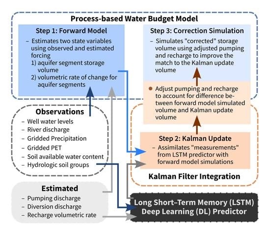
Figure 3 provides a schematic representation of the three-step integration process. Step one is forward model prediction, and step two is the Kalman update which combines “measurements” from the LSTM predictor with forward model predictions. Step three is the forward model correction. The Kalman filter update calculation for storage is analogous to the object tracking or position estimation implementation that is often provided as a Kalman filter implementation example [7,60]. Additional details of the Kalman filter calculation are provided in Appendix A.
The implementation used here requires the first two assimilation windows, i.e., the first two months, as initialization periods. After initialization, the predicted state covariance matrix can be calculated for the current assimilation window with Equation (4), where k denotes the current assimilation time window, is the previous assimilation time window, is the updated state covariance matrix from the previous assimilation window, and A is the state transition matrix. Q is the process noise covariance matrix and provides for incorporation of an observation error model into a Kalman filter implementation.
The Kalman gain, Equation (5), can be determined using , H which is the state to measurement matrix that converts measured values to state values, and R, which is the measurement covariance matrix. Kalman gain determines how the “measurement” will influence the updated system state estimate [7].
The updated system state, , can then be calculated using Equation (6), where is the predicted system state from the forward model and are the measurements predicted by the trained LSTM model. The term is the measurement residual, or innovation [60].
In Equation (6), the function of the Kalman gain, , is evident. It is the weight given to the measurements and current-state prediction, and it can be “tuned” to impact filter performance. If the variance of the measurement is small relative to variance of the prediction, then will be closer to one. When the variance of the prediction is small relative to the variance of the measurement, then will be closer to zero. A high gain means the filter places more weight on the most recent measurements, , and moves towards or conforms better with the recent measurements. Alternatively, low gain results in more movement towards or conformance with model predictions, . At the extremes, a gain close to one produces a “jumpy” trajectory; a gain close to zero smooths out noise but decreases filter responsiveness. When a really noisy measurement comes in to update the system state, the Kalman gain will trust the “predicted” state estimate more than the new, but inaccurate, measurement [6,7].
2.5. Goodness-of-Fit Metrics
Two commonly used goodness-of-fit measures for discharge hydrographs are (1) Nash–Sutcliffe efficiency (NSE) [61] and (2) Kling–Gupta efficiency (KGE) [62]. The NSE is defined in Equation (8) [61], where s is the simulated or calculated value and o is the observed or data value.
The KGE metric, see Equation (9), was developed through the decomposition of the NSE into the linear correlation coefficient between observed and simulated values, , a measure of relative variability in the simulated and observed values, , and a bias component, [62]. Both NSE and KGE range from to 1.0 with 1.0 representing a “perfect” match. In Equations (10)–(12), is the mean; is the standard deviation, and N is the number of observations.
A custom goodness-of-fit metric is used to compare predicted outcomes among trained, or “final”, models. This metric is the sum of NSE and KGE, from Equation (13). ranges from to 2.0 with 2.0 representing “perfect” fit.
NSE and KGE are traditionally used for time series goodness-of-fit comparison for sequences that have significant variability. For time series that vary slowly and rhythmically, such as groundwater elevations, other metrics such as root mean square error (RMSE) and normalized root mean square error (NRMSE) are typically used. The RMSE is defined in Equation (14). The NRMSE is the RMSE normalized by the range of observed values, o. Traditionally, a NRMSE less than 10% identifies an acceptable match of simulated to observed water level elevations in wells.
2.6. Data
Three distinct data types are employed in DL training, testing, and validation. Outcomes, or targets, provide known values for history matching. Water level elevations observed in five wells and river discharge observed at three stream gauging stations are the target data sets. These target data sets were used for calibration and validation of the UCUWCD Water Balance Model, and the LSTM model is trained to predict the target time series that were used in UCUWCD Water Balance Model “calibration-constrained uncertainty analyses [1,2]”.
Feature data sets provide the inputs from which the LSTM model learns to predict outcomes. Dynamic input data sets include river discharge at three “inflow” gauging stations on Figure 1, weather and climate parameters, and pumping and water rights diversions. Similar inputs are used for the UCUWCD Water Balance Model and the LSTM model because the goal of LSTM model development is to produce a DL predictor that predicts values for UCUWCD Water Balance Model calibration targets using inputs that are as alike as possible given the standardization requirements of DL feature preparation and the dimensional consistency requirements of process-based models.
The third data type is static watershed properties; these data provide static inputs, or features. In this study, static properties used in EA-LSTM models are derived from the parameterization of the UCUWCD Water Balance Model. Similar target, feature, and static data sets are used in the LSTM predictor and the UCUWCD Water Balance Model, which provides the base model for forward model development.
2.6.1. Water Level Observations in Wells
Time series of water levels observed in wells provide one type of target data set. Well elevation targets are used from the five wells shown on Figure 1. Only the J-27 well is a dedicated monitoring well; water is pumped from the other four wells. Each well is assumed to be an “index well” and thus provide an observation of the current volume of water in the aquifer using a look-up table to interpolate volume from the observed stage, i.e., the water level elevation observed in the well.
Table 5 provides information on these wells. The period of data coverage is limited for three wells (Willoughby, McBride #1, and McBride #3) to 10 to 12 months because of equipment malfunction. The “Start” date in Table 5 for Willoughby, McBride #1, Ehler, and McBride #3 wells denotes the approximate date of installation of automated logging equipment; the “End” date in Table 5 for Willoughby, McBride #1, and McBride #3 wells denotes the approximate date of equipment malfunction. After malfunction, no data were collected from these wells for several years. Water level elevations are observed in each well at daily or higher frequencies. Daily average water level observations are aggregated to monthly averaged water level targets.
As discussed in Section 2.4.1, DA approaches, including the Kalman filter, use an observation error model that represents uncertainty introduced from noisy data and limitations of the forward model. In Kalman filter implementation, the observation error model is a combination of Q in Equation (4) and R in Equation (5). Note that R in Equation (5) is constant during assimilation in this implementation, and there is no k subscript denoting an R term identified with a particular assimilation window. Q and R provide the observation error model because these are the two independent terms that affect the Kalman gain, , in Equation (5). As mentioned in Section 2.4.2, the Kalman gain can be “tuned” to impact filter performance.
An observation error model represents uncertainty from measurement error and representation error. Measurement error is expected to be significant for all index wells except for J-27 because J-27 is a monitoring well, and the other index wells are pumped with some unknown frequency. The “index well” assumption is that the water level observed in the well can be used as a staff gauge to interpolate water storage volume. If pumping occurs in an index well, then the water level observation is also measuring well efficiency and localized variations in water surface, and there is an expectation for significant measurement error.
The “index well” concept means that the water level elevation observed in the well represents a flat potentiometric surface that exists in a reservoir or bucket that is filled with granular material, i.e., porous media. It is unlikely that the potentiometric surface is truly flat because it is known that water is moving through the Uvalde Pool System and a gradient is required to drive this movement. It is also probable that porous media flow is not the most important flow process in this highly complex environment with highly transmissive pathways such as connected caves and regions of elevated secondary porosity from dissolution. Consequently, the expectation is for significant uncertainty related to differences between model assumptions and representations and what the water levels observed in the wells represent in terms of a measurement of volume of water in an aquifer segment.
Because there is significant uncertainty and limited data, see Table 5, Kalman filter implementation relies on Kalman gain tuning to produce a balance between forward model predictions and LSTM model measurements. Tuning provides a way to distribute the uncertainty from measurement and representation error between the forward model and the measurements.
2.6.2. River Discharge Observations
Discharge observations from six of the seven United States Geological Survey (USGS) gauging stations shown on Figure 1 provide either DL inputs or targets. Station ID 8196300 is not used in DL modeling, but is used in the forward model; this station is not used because it always provides a small observed discharge relative to Station ID 8195000 and thus provides minimal additional value for training and prediction. The “outflow” type denotes discharge observations which are used as targets for training and model skill assessment; the “inflow” type provides an observation of surface water inflow into the study area. Table A2, in Appendix B, provides summary characteristics for these gauging stations.
As mentioned in Section 2.3.3, a common-sense baseline is developed for discharge targets. A synthetically estimated, expected uncertainty envelope for stream discharge data sets, developed in Ref. [59], was used to generate the common-sense baseline for predicted discharge outcomes. The common-sense baseline is then used to (1) provide a lower threshold that needs to be exceeded for demonstration of model skill and (2) generate an upper threshold above which the model is assumed to be over-fitting and learning to reproduce measurement noise and calculation uncertainty.
Additional details of the baseline assessment calculation are provided in Appendix B. In the baseline assessment, a Monte Carlo model is used to generate realizations of synthetic discharge from the gauging station time series. Synthetic discharge is flow regime dependent and employs expected error estimates by flow regime from Ref. [63] of ±50–100% for low flows, ±10–20% for medium to high flows, and ±40% for out of bank high flows. A thousand realizations of synthetic discharge are generated using a biased normal variate to produce unique realizations of discharge that honor the expected error estimates in a stochastic sense. For each realization, goodness-of-fit metrics are calculated for the synthetic discharge realization and the observed discharge sequence.
Table 6 provides a summarizing statistical description of calculated goodness-of-fit metrics from common-sense baseline analysis. Maximum and minimum , from Equation (13), define the upper and lower thresholds for each target-gauging station. For example, the lower threshold for Station ID 8197500 is 1.1. When a DL model implementation equals or exceeds this threshold for the validation data set, it is assumed that the DL model demonstrates predictive skill. The upper threshold for this station is 1.7. DL models that equal or exceed this upper threshold for the validation data set are assumed to be equally good because it is assumed that models that exceed this threshold have learned to reproduce noise in the observation data set and are not generating additional predictive skill.
2.6.3. Weather and Climate Observations
Climate is the weather of a place averaged over across an interval of time [64]. Weather refers to the daily and higher frequency events occurring in the atmosphere [65]. Three-decade averages of weather measures, called climate normals, are frequently used to provide place- and period-specific climate description from weather observations [66].
For DL model training and implementation, deficit (D) values provide the weather parameter input. D is precipitation (P) depth minus the potential evapotranspiration () depth. D for LSTM model training is derived from the P and weather forcing data sets used in the UCUWCD Water Balance Model.
P and air temperature data sets were obtained from the Parameter Elevation Regressions on Independent Slopes Model (PRISM) Climate Group [67] on a 4 km grid for the study area (see Figure 1) and used to calculate D. Daily data are available from 1981 to present. These gridded meteorological data are derived, or interpolated, from thousands of point data collection stations using information in long-term precipitation climatologies and weather radar return patterns [68,69].
is calculated using the Hargreaves–Samani method, or the 1985 Hargreaves equation [70,71]. This method produces reference crop evapotranspiration () predictions for weekly or longer periods for use in regional planning, and is frequently used because of its simplicity, reliability, minimum data requirements, and ease of computation. It has been widely used in the US and globally when air temperature data are the only available weather parameter observations [70,72].
Climate normals for 1991–2020 derived for the study basin from PRISM data sets are provided in Figure 4. A negative D value is expected for every month because average , on a monthly basis, is always larger than average P, which denotes a water supply limitation on evapotranspiration.
2.6.4. Groundwater Pumping and Water Rights Diversions
Groundwater pumping and water rights diversions from streams and rivers are another input data set for DL model training and implementation. These are the primary removals of water from the regional water budget that are unrelated to processes in the terrestrial hydrologic cycle. Neither pumping nor diversion volume is directly observed for most extraction locations. Extractions, i.e., pumping and water rights extractions, are estimated based on permitted diversion and pumping volumes in conjunction with rough estimates for amounts that are exempt from permitting.
Table 7 provides the estimated distribution of annual pumping, by month, for Uvalde County, TX, empirically estimated by the EAA for use in resource management. Values in Table 7 are proportions of annual totals. It is assumed that water rights diversions follow the same annual pattern as pumping.
Annual volumetric estimates of diversion and pumping volume are used in conjunction with Table 7 to generate dimensionally consistent diversion and pumping time series used in the UCUWCD Water Balance Model. DL methods require input standardization, and the monthly percentages or proportions in Table 7 are used for standardized LSTM model inputs.
2.6.5. Soil Properties
A selection of watershed properties is used to develop static parameters for EA-LSTM implementation. These properties were extracted from the Soil Survey Geographic Database (SSURGO) mapping of the study area [73] during development of the UCUWCD Water Balance Model to parameterize previous watershed regions. In this model, soil properties were identified for 15 hydrologic response units (HRUs).
The two soil properties from the UCUWCD Water Balance Model that are used for static EA-LSTM properties are (1) available water capacity (AWC) and (2) hydrologic soil group (HSG) designation. There are four HSG types that are defined for each HRU. A single value of AWC, which is the area weighted average of all soil layers, is used for each HRU. Five properties for 15 HRUs are 75 static watershed properties.
AWC is the volume of water that should be available to plants if the soil, inclusive of fragments, were at field capacity. It is commonly estimated as the amount of water held between field capacity and wilting point, with corrections for salinity, fragments, and rooting depth [74].
HSGs are based on estimates of runoff potential made by soil scientists as part of soil-mapping procedures. Soils are assigned to one of four groups (A, B, C, or D) according to the rate of water infiltration when the soils are not protected by vegetation, are thoroughly wet, and receive precipitation from long storms. HSG A soils have low runoff potential when thoroughly wet, and water is transmitted freely through the soil so that the infiltration and percolation potential is high. HSG B soils have moderately low runoff potential when thoroughly wet and water transmission through the soil is unimpeded. HSG C are soils that have a slow rate of infiltration and transmission when thoroughly wet; HSG D soils have a very slow infiltration and transmission rate when thoroughly wet and thus have a high runoff potential [75].
3. Results
Results were generated from the training and validation of the LSTM model that projects time series values for the UCUWCD Water Balance Model calibration targets. LSTM projections of water levels in index wells provide “measured” values for Kalman filter updates and provide predicted water level values prior to installation of monitoring equipment and after equipment malfunction. LSTM model results are discussed in Section 3.1. Results related to the Kalman filter integration of LSTM predictor “measurements” to forward model simulations are provided in Section 3.2.
3.1. Trained and Partially Validated Complex Graph LSTM Predictor
Table 4 identifies three different groups of targets, or outcomes, for LSTM training. These three groups are delineated by the length and coverage of the available data sets for training.
- “Outflow” discharge from gauging stations 8197500, 819200, and 8204005;
- Data coverage 1 January 2003 to 31 November 2019;
- J-27 well water level elevations;
- Data coverage 31 January 2014 to 31 October 2019;
- “Other Wells,” Ehler, Willoughby, McBride Well #1, and McBride Well #2, water level elevations;
- Data coverage 27 October 2017 to 13 August 2018;
Three separate LSTM models, one for each target group, were created and trained to maximize the data availability for each target group. The “Other Wells” group has insufficient data for independent validation; this is a concern for the generalization ability of the “Other Wells” LSTM model.
After independent training and validation, the three LSTM models were combined into a single complex graph model as shown in Figure 5, which is the LSTM predictor. The LSTM predictor is considered as partially validated because insufficient outcome data were available to validate the “Other Wells” LSTM model.
The complex graph LSTM predictor projects index well water level outcomes used as “measurements” in the Kalman filter integration approach shown on Figure 3. The LSTM predictor takes one set of inputs and routes copies of the inputs to each sub-model and produces eight outputs or predicted outcomes. Three of the eight outputs are discharge outputs, which are not used in the Kalman filter integration. The remaining five outputs are well water level outputs for the wells described in Table 5.
Table 8 presents a comparison of goodness-of-fit metrics across the UCUWCD Water Balance Model, the forward model, and the LSTM predictor. The goodness-of-fit metrics for the LSTM predictor are significantly better, relative to the other two models, for the index wells. However, the “Other Wells” grouping is likely over-fit because there were insufficient data for independent validation. Sufficient data for independent validation does exist for the J-27 well. The goodness-of-fit metrics for J-27 identify skill in predicting water level outcomes.
Goodness-of-fit metrics for discharge targets are similar between the UCUWCD Water Balance Model and the LSTM predictor. The comparison of Table 8 to Table 6 suggests that the LSTM predictor is probably over-fitting at Station ID 8197500 because is a “perfect” 2.0, and the upper threshold in Table 6 is 1.7. The observed discharge at 8197500 is zero for the entire 291 day validation period listed on Table 4. Consequently, it is difficult to determine how much skill the LSTM predictor has for this station. For Station ID 8192000, validation is 1.5, which is between the lower threshold value of 1.1 and upper threshold value of 1.6 in Table 6. Validation is 1.3 for Station ID 8204005, which is between the lower threshold value of 0.9 and upper threshold value of 1.4.
3.2. Kalman Filter Integrated Water Balance Results
The goal of this study is to use DA to integrate DL model predictions to a process-based water budget calculation. A Kalman filter implementation provides DA integration. The LSTM predictor from Section 3.1 provides DL model predictions which are integrated to the process-based forward model. Kalman filter integration is implemented as shown in Figure 3. The forward model provides the predicted values, , and the LSTM predictor from Section 3.1 generates the measured values, . The Kalman filter calculates the dynamic Kalman gain using Equation (5), and the Kalman gain is used, along with and , to generate the Kalman update, , which is a weighted combination of and .
The Kalman update cannot be used directly as a predicted value for the forward model without violating the inherent mass balance in the process-based water budget calculations. Consequently, pumping and recharge are adjusted to cover the difference between the Kalman update and the initially predicted value. The forward model is then re-run for the last assimilation window using adjusted pumping and recharge. The UCUWCD Water Balance Model is a network model that has many different linkages (see Table 1) and there is no guarantee that updating one or two components of the water budget will lead directly to the desired predicted value, i.e., a predicted value from the “correction” assimilation window that exactly matches the Kalman update value.
Manual Kalman gain tuning was utilized to generate Kalman filter updated water balance model results that seemed to subjectively “best” capture the observed water levels cast to aquifer segment storage volume. The goal of the subjective, manual exercise was to capture the observed storage volume values within the envelope provided by the Kalman update ± three standard deviations, or . This six range is assumed to provide a 95% confidence interval (CI). values are listed in Appendix A, Table A1. Additional information on tuning and “best” Kalman gain tuning-related values is provided in Appendix A.3.
Figure 6 displays the evolution of Kalman gain values across simulation time, after tuning, for the five aquifer segments. Note that a Kalman gain and filter update are not calculated for the first two assimilation windows, i.e., the first two months. The first two months are required to initialize the calculation matrices. The Kalman update simulation uses the same time parameters as the UCUWCD Water Balance Model and the forward model. The simulation duration is 1 January 2016 through 30 September 2019, with a daily time step. The assimilation window for the Kalman filter update application is monthly.
Table 9 lists the Kalman gain values at two selected time points: (1) October 2017, which is the point when there are two years left in the simulation and gain values for most of the aquifer segments are leveling off, and (2) September 2019, which is end of the simulation. Volumetric results from the Kalman filter implementation are presented for the two-year period from 1 October 2017 through 30 September 2019 in order to present simulated values after most gain value evolution occurs.
Storage-related results are shown from the Kalman filter-integrated or combined calculations are compared to the forward model and LSTM predictions for the Edwards and Austin aquifer segments on Figure 7 and Figure 8, respectively. Equivalent figures for Buda #1, Leona Gravels, and the Buda #2 aquifer segments are provided in Figure A3, Figure A4 and Figure A5 in Appendix C. In these five figures, all “Observations” and “LSTM Measurements” fall within the 95% CI.
Pumping volume, a removal or extraction of water from the aquifer segments, and recharge volume, an addition of water to the aquifer segments, are dynamically updated in the Kalman filter integration to attempt to have the updated forward model, after the “correction” step, produce the Kalman update volume, , at the end of the re-simulation of the previous assimilation window. Figure 9 and Figure 10 display volumetric adjustments to pumping and recharge across simulation time for the Edwards and Austin aquifer segments, respectively. Volumetric adjustments to Buda #1, Leona Gravels, and Buda #2 aquifer segments are shown in Figure A6, Figure A7 and Figure A8 in Appendix C. No adjustments to Edwards aquifer segment recharge were required as part of Kalman filter integration, as shown in Figure 9. Table 10 summarizes the volume adjustments made to each aquifer segment during the simulation presentation period of 1 October 2017 through 30 September 2019.
4. Discussion
DA provides methods for incorporating observations, or data, with numerical models. In this study, assimilated data are LSTM model predictions of the water level in five wells. Three of the five target wells, Willoughby, McBride #1, and McBride #3, have observations for only about 11 months. Observations are also available for a limited period, about 31 months, for a fourth target well, the Ehler well. Limited observations for these four wells means that there are insufficient data for training, testing, and validation and that the LSTM predictor is likely over-fitting estimates for these four wells, as discussed in Section 3.1. Over-fitting is when a statistical learning predictor learns to reproduce inherent noise and systematic error in a data set in addition to “true” physical trends.
The fifth target well, J-27, is a monitoring well and has a relatively long record of observation as identified in Table 5. Sufficient data are available for training, testing, and validation of the J-27 well. Because about 14% of the J-27 data set (see Table 2) was reserved for independent validation and because the LSTM predictor demonstrates skill in predicting J-27 water levels during the independent validation period (see Table 8), the J-27 portion of the complex graph LSTM predictor demonstrates generalization ability.
The Kalman filter integration combines the LSTM predictor “measurement” with the process-based water budget forward model prediction by weighting the “measurement” and the prediction with the dynamically evolving Kalman gain. The relative magnitude of the prediction variance to the “measurement” variance is used in determining the Kalman gain. The Kalman gain is external to or independent of LSTM predictor generalization ability, which is analyzed only in relation to the noisy and uncertain outcome data set used for training and validation, and it assimilates information from the process-based water budget model that is not available to the LSTM predictor.
The LSTM predictor projects water level elevation for the Edwards aquifer segment using the J-27 output, and Table 9 lists a relatively small Kalman gain value for the Edwards aquifer segment. A Kalman gain value close to zero, such as 0.087 for the Edwards aquifer segment, denotes a relatively large variance for forward model predictions and provides more weight to forward model predictions, even though analysis of J-27 LSTM predictions, relative to solely water level outcomes, suggest generalizability. In contrast, Table 9 identifies Kalman gain values of 0.624 and 0.673 for the Leona Gravels aquifer segment (Ehler index well) and the Buda #2 aquifer segment (McBride #3 index well), respectively. Kalman gain values closer to one provide more weight to LSTM predictor estimates in assimilation, even though it is expected that the LSTM predictor for the Ehler and Buda #2 water levels is over-fit and is producing biased estimates, corrupted by noise and error in the limited observation record used to train the “Other Wells” LSTM predictor.
An individual LSTM predictor was created for the J-27 well (see Figure 5) to leverage data availability for training, testing, and validation of this well. A complex graph LSTM predictor, see Figure 5, was then created to combine individual LSTM predictors so that the J-27 and river discharge model could trained with relatively long records of observations and could be subjected to independent validation. The primary means to improve a DL model is to train it on more and better data [28], and statistical learning approaches assume and require that training, testing, and validation data sets are clean and “perfect”.
Hydrological data sets tend to be noisy, contain rare occurrences or extreme events, and be estimates of a desired parameter value from a different type of observation. Calculated potential evapotranspiration from observed temperature, estimated river discharge from observed stage, and calculated aquifer volume from index well stage are three commonly used, derived hydrologic data sets. A common-sense baseline, see Section 2.3.3, can be used with outcome or target data sets that are known to be noisy and contain errors to assess statistical learning generalization ability. However, this assessment of generalizability is limited to the outcome data set used in training and its inherent flaws. In this study, a common-sense baseline is generated for the river discharge LSTM predictor (see Figure 5) that provides two thresholds: (1) a lower threshold that needs to be exceeded for demonstration of model skill and (2) an upper threshold. above which the model is assumed to be over-fitting.
DA, in contrast to statistical learning methods, does not require data perfection and provides for the explicit representation of expected measurement error in target observations through an observation error model, see Section 2.4.1. An observation error model is employed for aquifer segment storage in this study. Measurements of water level stage in wells are transformed to volumes using the storage volume description within the forward model. The LSTM predictor provides the water level stage measurements that are assimilated by the Kalman filter-integrated water-balance approach. Integration of the LSTM predictor allows application of the observation error model to LSTM predictions and accounts for inherent target uncertainty and system representation uncertainty externally to the statistical learning algorithm.
The Kalman filter-based integrated LSTM predictor and process-based water budget calculation presented here is a three-step implementation that employs existing models and computer programs, with minimal modification, in the unique configuration explained in Figure 3. Step one is the prediction of current aquifer segment storage with the forward model. Step two is the generation of the Kalman update aquifer segment storage through combination of LSTM predicted water levels, converted to aquifer segment storage, with forward model predicted storage using Kalman gain weighting. Step three is the “correction” step where the unobserved pumping and diversion volume are adjusted for the previous assimilation window, and the forward model is re-run with adjusted pumping and diversion discharge to predict current aquifer segment storage that approximates the Kalman update storage.
The forward model and the LSTM predictor are separate models and only the inputs to the forward model are adjusted. The forward model provides a water budget calculation where the budget framework enforces mass conservation. Because the LSTM predicted stage is used only to calculate the Kalman update storage and because pumping and diversion discharge are updated to account for the residual between step two storage and step one storage, the Kalman filter-integrated water balance is inherently mass conservative, even though it leverages statistical learning predictions for which mass conservation is undefined.
EnKF approaches have been extended previously with one or more “corrector” update steps to enforce water budget closure. Ref. [11] incorporated constraints to the EnKF and applied a constrained EnKF in a two-step process to estimate a terrestrial water budget across the southern Great Plains region of the United States (US). Step one in this estimation is the standard EnKF, and step two is a constraint step that optimally redistributes water budget imbalance created in step one to adjust or correct the budget calculation. Ref. [25] produced a two update, weakly constrained EnKF approach that enforces water balance closure and accounts for data uncertainty and applied it to assimilate gravity recovery and climate experiment (GRACE) terrestrial water storage observations with a global-scale hydrological model. This two-update, weakly constrained EnKF was subsequently modified to incorporate a more general, unsupervised framework that permits an unknown water-balance model covariance [26], and the unsupervised and modified framework was applied for combined assimilation–calibration [27]. These previous EnKF “corrector” applications are conceptually similar in implementation (but at disparate scales, and using different types of data sets that are observed, and which do not employ statistical learning predictions) to the three-step implementation in this study.
4.1. Integrated Volume Calculation—Advantages and Limitations
Kalman filters are a DA algorithm with the goal of continuously updating numerical model results to represent observations, and are frequently employed in active, “operational” environments with real-time or near real-time updates to optimize assembly line performance, track objects, and implement autonomous vehicle navigation and control [6,7]. Given the goal of continuous improvement, it only makes sense to use a classical Kalman filter implementation for “active” and rapid fusion of data with numerical models. In other words, a Kalman filter is not a “calibration” technique but is a technique for continuous optimization of dynamic system representation.
Here, Kalman filter integration produces an operations-focused water budget calculation that continuously evolves as additional data are acquired and that works with the state variables of water storage volume and rate of change of storage. The volume of water that is stored and volumetric additions to and extractions from storage are the primary concerns for resource management and conservation. The volume of water stored in the five aquifer segments in this study is an unobserved quantity. The explicit focus on storage volume and the adjustment of uncertain discharges allows for resource planning using Equation (1) and the concept of residence time, .
The main advantages of Kalman filter integration of DL predictions to a process-based water budget involve leveraging the advantages of each disparate approach, i.e., DL versus process-based approaches, to compensate for the deficiencies in the other approach. Disadvantages of process-based water budget calculations include: (1) model parameterization and process representation complexity increases with site complexity, which means that significantly more effort is required to make a water budget calculation for a physically complex site than for a simple site, and (2) model inputs and outputs must have dimensions and must balance dimensionally, which means that dimensionless, or proportional, soft information is difficult to employ within purely deterministic implementations of these models. Statistical learning advantages directly ameliorate the disadvantages of process-based calculations and include that (1) site complexity is uncoupled from DL model complexity so that there is no additional effort required for complex sites relative to simple sites and (2) dimensionless trends can be used as features, or inputs, as is utilized for pumping and water rights extractions in this study.
Similarly, the deficiencies of DL approaches are counterbalanced by the advantages of process-based approaches. Disadvantages of DL models include: (1) dimensionless and standardized inputs and outputs means no mass conservation or dimensionally consistent representation, which can lead to allocating too much importance to trivial correlations, and (2) standardization requires assumption of weak stationarity, which means that weak stationarity among training inputs and prediction inputs must be assumed. Contrasting advantages of process-based water budget calculations are: (1) explicit calculation of volume of water in storage, (2) physical process representation provides for representation of process function outside of the range of calibration data, and (3) inherent mass conservation and dimensional consistency as part of the budget, or balance, framework.
Kalman filter integration of these two fundamentally different approaches generates further advantages of (1) working directly with the unobserved state variable of water storage volume, (2) ability to combine dimensionless predictions of aquifer stage with the process-based volume description when stage observations are limited or unavailable, and (3) use of dimensionless extraction trends as inputs to predict aquifer stage in the LSTM predictor allows for “correction” of these unobserved, and uncertain, volumetric extractions and additions in the process-based model to yield “optimal” storage volume solutions.
The main limitations of the Kalman filter integration are: (1) it does not create new observations but merely spreads the uncertainty in previously observed values among the state variables of storage volume and rate of change in storage volume and (2) it is active, evolutional, and requires the continuous acquisition of additional observations to promote evolution and ongoing representation enhancement. If additional observations, i.e., additional data collection, are not planned, then using an active and evolutional approach is a waste of time because no new observations are available for the continued improvement of system state representation.
4.2. Future Work
The future work goal for this study is to implement this type of operational DA of DL predictions to process-based water budgets in an environment of continuous improvement via continuous acquisition of new observations analogous to assembly line function and process optimization for manufacturing. The LSTM predictor does not create “new” observations. It only estimates water level values based on learning from a limited set of observations. Consequently, the immediate need for future advancement in the current study area is to remedy mechanical issues with observation collection equipment so that new observations can be, and are, obtained.
Additional observations can be directly incorporated as “measurements” as soon as they are available, and the LSTM predictor should only be used when observations are not available. More data, and continual collections of observations, will allow for examination of different distributions of the residual volume correction (from Figure 3) between pumping and recharge. The correction volume distribution between pumping and recharge, used in this study, was arbitrarily derived to enable process-based and mass-conservative correction of the water budget calculation. Additional observations will eventually allow for iterative cycles of model development and optimization as part of the ongoing improvement to dynamic system representation.
Iterative cycles of model development will include both the process-based forward model and the LSTM predictor. An LSTM predictor should be re-trained and the updated representation validated whenever there are one to two years of additional data. The process-based forward model should be re-calibrated as part of this cycle of model optimization; additional complexity should be incrementally introduced to the process-based model as suggested by analysis of new observations. Finally, the process-based model will eventually need to be changed to a systems dynamics model that can inherently represent complex and interrelated water demands like feedback loops. The current process-based model is only capable of hydrologic routing, one-way movement of water across the interconnected aquifer and river segments, with a limit of five outflows.
5. Conclusions
LSTM-predicted water levels in wells are integrated to a process-based, mass-conservative water budget framework via classic Kalman filter DA. The integrated calculation is a three-step combination of a process-based water balance model, which is the forward model, with a DL predictor. The volume of water stored in aquifer segments is the important system state tracked in the assimilation.
In the first step, the forward model predicts aquifer storage volume. A Kalman filter calculates an updated aquifer storage volume by assimilating “measurements” from an LSTM predictor, predicted using similar inputs to the forward model, with initial forward model predictions in the second step. The final calculation step utilizes modified pumping and recharge inputs, adjusted to address the difference between the Kalman filter update and the forward model prediction, to recalculate the water budget for the current assimilation window in a “correction” step. Neither pumping nor recharge is observed in the study area, and values used in the prediction step, i.e., step one, are approximate.
This Kalman filter integration provides advantages of working directly with the unobserved state variable of water storage volume and combining dimensionless predictions of aquifer stage from the LSTM predictor with the process-based volume description for the water budget model in a mass-conservative fashion. It generates an operations-focused water budget calculation that provides for optimal system representation conditional upon existing observations and that can continuously evolve and improve as additional data are acquired.
DL requires clean and consistent data because statistical learning focuses solely on learning correlations from standardized data sets. Significant uncertainty issues are known to impact the target, or outcome, data sets used to train and validate the LSTM predictor in this study. A common-sense baseline is employed to facilitate interpretation of LSTM model generalizability accounting for uncertainty in river discharge observations. DA, in contrast to statistical learning, provides for explicit incorporation of target data set uncertainty including measurement error through the observation error model. An observation error model is used for the storage state variable in the integrated calculation to externally address data uncertainty impacts to LSTM predictions and to incorporate additional uncertainty inherent in the dynamic system representation of the water budget model.
Funding
This research was funded by Southwest Research Institute, Internal Research and Development Grant 15-R6209.
Institutional Review Board Statement
Not applicable.
Informed Consent Statement
Not applicable.
Data Availability Statement
Not applicable.
Acknowledgments
The author wishes to acknowledge the contributions of three anonymous reviewers whose comments and suggestions improved the quality of this paper.
Conflicts of Interest
The author declares no conflict of interest.
Abbreviations
The following abbreviations are used in this manuscript:
| AI | Artificial intelligence |
| AWC | Available water capacity |
| CI | Confidence interval |
| DA | Data assimilation |
| DL | Deep learning |
| EA-LSTM | Entity-aware long short-term memory |
| EAA | Edwards Aquifer Authority |
| EnKF | Ensemble Kalman filter |
| FDC | Flow duration curve |
| GRACE | Gravity Recovery and Climate Experiment |
| HRU | Hydrologic response units |
| HSG | Hydrologic soil group |
| HSPF | Hydrological simulation program—FORTRAN |
| KGE | Kling-Gupta Efficiency |
| LSTM | Long short-term memory |
| MAE | Mean absolute error |
| ML | Machine learning |
| MSE | Mean square error |
| NRMSE | Normalized root mean square error |
| NSE | Nash-Sutcliffe Efficiency |
| ODE | Ordinary differential equation |
| PDE | Partial differential equation |
| PRISM | Parameter-Elevation Regressions on Independent Slopes Model |
| RMSE | Root mean square error |
| RNN | Recurrent neural network |
| SPI | Standardized precipitation index |
| SPEI | Standardized precipitation evapotranspiration index |
| SSURGO | Soil Survey Geographic Database |
| SWAT2012 | Soil and Water Assessment Tool 2012 |
| TX | Texas |
| UCUWCD | Uvalde County Underground Water Conservation District |
| US | United States |
| USGS | United States Geological Survey |
Appendix A. Definitions and Equations for Kalman Filter Implementation
Appendix A.1. Definitions
The Kalman filter implementation presented here is formulated to use measured and projected water level elevations in “index wells” to calculate aquifer segment water storage volume. The means for calculating volume from water level elevation is the FTABLE in the UCUWCD Water Balance Model. The FTABLE provides mapping from volume to water level elevation for the RCHRES structure.
There are five aquifer segments or sub-component aquifers in this analysis. The state variables are volume, v, for each aquifer and rate of change in volume, , across the current assimilation window, Equation (A1). k denotes the time index for the ending time of the current assimilation window, . denotes the time index for the ending time of the previous assimilation window, .
In Equation (6), is the vector of predicted states produced by the forward model for the current assimilation time window, k. Equation (A3) provides definition of . The subscripts identify the aquifer segment according to the list below.
- 1: Edwards R001 from Table 1;
- 2: Buda #1 R002 from Table 1;
- 3: Austin R003 from Table 1;
- 9: Leona Gravels R009 from Table 1;
- 10: Buda #2 R010 from Table 1;
In Equation (6), is the vector of projected states for the current assimilation window, k, produced by the trained LSTM model. The LSTM model produces water level elevations in the index wells, which are converted from water level elevations to volume values using the corresponding FTABLE. Equation (A4) provides the definition of ; note this is the same as Equation (A3); however, the sources are different. are predicted by the forward model, and are projected by the LSTM predictor.
Appendix A.2. Equations
- A is the state transition matrix, Equation (A5);
- Q is the process noise covariance matrix that provides the observation error model, Equation (A6);
Because the transform from water level elevation to volume is executed external to the Kalman filter implementation, the main diagonal of A is ones.
In Q, the standard deviation, , of volume provides the observation error model. The volume sequences, from which the standard deviations are calculated, are projected by the LSTM predictor across the full available input feature period of 1 February 2003 through 31 December 2019 for LSTM training because no index wells are included in the inputs.
- H is the state to measurement matrix, Equation (A7);
- R is the measurement covariance matrix, Equation (A8);
Because the transformation to volume is handled externally to the Kalman filter algorithm, The H terms for indices one through five, which correspond to the volumes, are one as shown in Equation (A7). The indices, six through ten, are set to zero because the rate of change of volume is an “unobserved state” that is tracked as part of Kalman filter implementation.
R in Equation (A8) is the initial measurement covariance matrix. This matrix is modified to tune the Kalman gain as discussed in Appendix A.3. The U term in Equation (A8) is an arbitrarily selected large number (8 × 10 in this implementation) that represents a guess at initial hidden state uncertainty.
Table A1 provides the standard deviation, , values used to calculate the initial versions of the Q and R matrices in Equations (A6) and (A8).

Table A1.
Standard deviation values used in initial R and Q matrix creation.
| Aquifer | Reservoir | Standard Deviation | Prediction | |
|---|---|---|---|---|
| Segment | ID | Mm | % of Edwards | Period 1 |
| Edwards | R001 | 40.9 | 100 | 1 February 2003 to 31 December 2019 |
| Buda #1 | R002 | 4.1 | 10.1 | 1 February 2003 to 31 December 2019 |
| Austin | R003 | 47.4 | 116 | 1 February 2003 to 31 December 2019 |
| Leona Gravels | R009 | 2.1 | 5.2 | 1 February 2003 to 31 December 2019 |
| Buda #2 | R010 | 1.5 | 3.6 | 1 February 2003 to 31 December 2019 |
1 Standard deviation values were calculated from the complex graph, trained LSTM model predictions across 1 February 2003 to 31 December 2019. The LSTM model predicts water levels in index wells. These elevations were converted to volume values using the FTABLES in the UCUWCD Water Balance Model.
Appendix A.3. Kalman Gain Tuning
In Table 8, the forward model produces NRMSE values greater than 10% for all five index wells and does not do a “good” job of predicting water levels. The LSTM predictor does, however, produce NRMSE values of less than 6% for all five index wells. Because the observation record was short (less than 14 months) for four of the five index wells, the LSTM predictor for these four index wells could not be both trained and validated on independent sets of outcomes. It is probable that the LSTM predictor for these four index wells is over-fitting. Over-fitting is when the model learns patterns that are specific to the training data but that are misleading or irrelevant when it comes to new data [28].
A manual, trial and error Kalman gain tuning exercise was utilized to generate Kalman filter updated water balance model results that seemed to subjectively best capture the observed water levels cast to aquifer segment storage volume. The goal of the subjective, manual exercise was to capture most of the observed storage volume values within the envelope provided by the Kalman filter updated water balance predictions . The range is assumed to provide a 95% confidence interval (CI). values are shown in Table A1. For Kalman gain tuning, modified versions of the Q and R matrices are employed. Equation (A9) shows the modified Q, or , representation used for tuning. In this equation, the q’s are aquifer segment unique multipliers.
Final tuned values for the q’s are listed below.
- ;
- ;
- ;
- ;
- ;
Equation (A10) shows the modified R, or , representation used for tuning. In this equation, the r’s are aquifer segment unique multipliers.
Final tuned values for the r’s are listed below.
- ;
- ;
- ;
- ;
- ;
Appendix B. Gauging Station Metadata and Discharge Statistics
Tables and figures describing stream gauging station metadata and statistical analysis are included in this appendix. At all gauging stations in Table A2 and on Figure 1, water stage recorders are used to measure water depth. A derived rating curve, unique to the gauging station, provides the translation from measured water depth to an estimated discharge. Stage measurement combined with estimation of discharge using a rating curve provides a calculated, or modeled, estimate of discharge rather than a direct observation. Discharge estimates from the gauges in Table A2 contain measurement and model error with an expectation for larger errors relative to direct observations of discharge.
The purpose of discharge statistical analysis is to develop a common-sense baseline for discharge targets following Ref. [59]. It is important for representation of the study site that the common-sense baseline incorporate relative uncertainty expectations between low flow and medium to high flow regimes. Ref. [63] provides flow regime dependent, expected error estimates of ±50–100% for low flows, ±10–20% for medium to high flows, and ±40% for out of bank high flows for discharge calculated using a stage measurement combined with a rating curve. Consequently, the largest relative uncertainty is expected for gauge records that are dominated by relatively low discharges.
Low flows are important in study site representation because the study area contains the BFZ Edwards Aquifer Recharge Zone, “Recharge Zone”, shown on Figure 1. Significant seepage losses are observed from the Nueces and Frio Rivers across the Recharge Zone using pairs of gauging stations. The upstream member of the pair provides observed discharge prior to the Recharge Zone; Station ID 8190000 is the upstream member for the Nueces River pair, and 8195000 is the upstream member for the Frio River pair. Station ID 8197500 is the downstream member for the Frio River, and 8192000 is the downstream member for the Nueces River. Differencing of the upstream member from the downstream member provides an estimate of seepage losses across the Recharge Zone.
Flow duration curves (FDCs) are used to graphically portray differences in discharge characteristics observed between the upstream and downstream members and to identify flow regime thresholds. An FDC represents the relationship between the magnitude and frequency of daily, in this case although weekly or monthly intervals could be used, discharge for a particular river basin and provide estimates of the percentage of time a given discharge was equaled or exceeded over a historical period [76]. Table A3 lists flow regime thresholds identified using an FDC for each gauging station.
Figure A1 provides FDCs for 8195000 (upstream Frio River) and 8197500 (downstream Frio River) along with flow regime threshold estimates. Discharge observed at the downstream 8197500 station is almost always smaller than that observed at the upstream 8195000 stations, even though the contributing area for 8197500 is 526 km2 larger, because of seepage losses. FDCs and flow regime estimates for the Nueces River upstream versus downstream stations are shown on Figure A2 and similar seepage loss patterns are evident in this figure because discharge observed at the downstream station, 8192000, is generally smaller than that observed at the upstream station, 8190000. Table A3 provides a summary of the pertinent flow indices calculated from these FDCs.
On Figure 1, the “inflow” type provides description of water inflow into the study area and identifies the upstream member of a seepage loss calculation pair. These “inflow” gauging stations are used as features or inputs for LSTM training and prediction. Station IDs 8195000 on the Frio River, 8190000 on the Nueces River, and 8190500 on the West Nueces River are the discharge features.
Downstream members are “outflow” stations and provide targets. Station IDs 8197500 on the Frio River, 8192000 on the Nueces River, and 8204005 on the Leona River are the discharge targets. Station ID 8204005 is the only station available on the Leona River and is not a member of a seepage loss calculation pair.
As shown in Table A3, the downstream members of the seepage loss identification pairs, 8197500 and 8192000, have 70th percentile discharges that are significantly smaller than the upstream pair member. Both the 70th percentile and 20th percentile probability of exceedance discharges are zero for 8197500 in Table A3, and the MDF of 1.0 -days has an exceedance probability of about 4.7%. The expectation is for zero discharge over 90% of the time at station 8197500.
Table A2.
Gauging Station Metadata.
| Station ID 1,2 | River | Description | Start of Record | Contributing Area km | Count (N) 3 | Type 4 |
|---|---|---|---|---|---|---|
| 8197500 | Frio | Frio Rv bl Dry Frio Rv nr Uvalde, TX | 1 October 1953 | 1634 | 24,837 | Outflow |
| 8195000 | Frio | Frio Rv at Concan, TX | 30 September 1924 | 1008 | 24,837 | Inflow |
| 8190000 | Nueces | Nueces Rv at Laguna, TX | 1 September 1952 | 1909 | 24,837 | Inflow |
| 8190500 | West Nueces | W Nueces Rv nr Brackettville, TX | 28 September 1939 | 1797 | 24,016 | Inflow |
| 8192000 | Nueces | Nueces Rv bl Uvalde, TX | 5 April 1939 | 4820 | 24,837 | Outflow |
| 8204005 | Leona | Leona Rv nr Uvalde, TX | 1 March 2003 | 342 | 6881 | Outflow |
1 Discharge data and gauging information come from United States Geological Survey (USGS), https://waterdata.usgs.gov/tx/nwis/rt (accessed on 23 June 2022). 2 All gauging stations are water-stage recorders. 3 31 December 2021 is the end date for all records for this analysis, and data are available through the present. “Count” is the count of days that have observations available from 1 January 1954 through 31 December 2021. 4 Type denotes whether a gauging station observes inflow to or outflow from the study domain shown on Figure 1.
Table A3.
Flow duration curve (FDC) analysis results.
| Station ID | Mean Daily Flow (MDF) 1 | 70th Percentile Threshold 2 | 20th Percentile Threshold 3 | 2nd Percentile Threshold 4 | Maximum Observed Discharge | Daily Standard Deviation | Monthly Standard Deviation |
|---|---|---|---|---|---|---|---|
| m/s-days | m/s-days | m/s-days | m/s-days | m/s-days | m/s-days | m/s-months | |
| 8197500 | 1.04 | 0.00 | 0.00 | 7.05 | 915 | 15.1 | 4.4 |
| 8195000 | 3.62 | 1.33 | 4.07 | 16.37 | 699 | 12.3 | 5.1 |
| 8190000 | 4.97 | 1.59 | 5.18 | 22.50 | 1991 | 24.2 | 8.6 |
| 8190500 | 1.02 | 0.00 | 0.08 | 4.73 | 1203 | 17.3 | 4.8 |
| 8192000 | 4.48 | 0.40 | 3.49 | 22.99 | 1461 | 34.2 | 12.6 |
| 8204005 | 0.82 | 0.00 | 1.17 | 2.39 | 411 | 7.4 | 2.2 |
1 Mean daily flow (MDF) provides the upper limit for low flow indices [77]. 2 The flow duration curve (FDC) 70th percentile threshold is a commonly used low flow index [77]. 3 The 20th percentile is a threshold for high to medium flows [78]. 4 The 2nd percentile is the threshold used for out of bank, high flows [78] in this study.
Figure A1.
FDC for 2 Frio River stations.

Figure A2.
FDC for 3 Nueces River stations.

Appendix C. Additional Kalman Filter Results
Figure A3.
Simulation Results for Buda #1 Aquifer Segment.

Figure A4.
Simulation Results for Leona Gravels Aquifer Segment.

Figure A5.
Simulation Results for Buda #2 Aquifer Segment.

Figure A6.
Pumping and Recharge Adjustments to Implement Forward Model Correction for the Buda #1 Aquifer Segment.
Figure A6.
Pumping and Recharge Adjustments to Implement Forward Model Correction for the Buda #1 Aquifer Segment.

Figure A7.
Pumping and Recharge Adjustments to Implement Forward Model Correction for the Leona Gravels Aquifer Segment.
Figure A7.
Pumping and Recharge Adjustments to Implement Forward Model Correction for the Leona Gravels Aquifer Segment.

Figure A8.
Pumping and Recharge Adjustments to Implement Forward Model Correction for the Buda #2 Aquifer Segment.
Figure A8.
Pumping and Recharge Adjustments to Implement Forward Model Correction for the Buda #2 Aquifer Segment.

Appendix D. Model and Source Code Availability
Models and associated “new” source code are available from the project GitHub repository. Available online at https://github.com/nmartin198/kfint_watbudg_lstm (accessed on 9 May 2023).
References
- Doherty, J. Calibration and Uncertainty Analysis for Complex Environmental Models. PEST: Complete Theory and What It Means for Modelling the Real World; Watermark Numerical Computing: Brisbane, Australia, 2015. [Google Scholar]
- Pest++ Development Team. PEST++: Software Suite for Parameter Estimation, Uncertainty Quantification, Management Optimization, and Sensitivity Analysis, Version 5.1.18. User Manual. 2022. Available online: https://github.com/usgs/pestpp (accessed on 24 October 2022).
- Evensen, G.; Vossepoel, F.; van Leeuwen, P.J. Data Assimilation Fundamentals: A Unified Formulation of the State and Parameter Estimation Problem; Springer: Cham, Switzerland, 2022. [Google Scholar]
- Kalman, R.E. A New Approach to Linear Filtering and Prediction Problems. J. Basic Eng. 1960, 82, 35–45. [Google Scholar] [CrossRef] [Green Version]
- Humpherys, J.; Redd, P.; West, J. A Fresh Look at the Kalman Filter. SIAM Rev. 2012, 54, 801–823. [Google Scholar] [CrossRef] [Green Version]
- Wikipedia Contributors. Kalman Filter. 2023. Page Version ID: 1144765839. Available online: https://en.wikipedia.org/w/index.php?title=Kalman_filter&oldid=1144765839 (accessed on 27 March 2023).
- Franklin, W. Kalman Filter Made Easy: A Beginners Guide to the Kalman Filter and Extended Kalman Filter with Real Life Examples Supported by Python Source Code. Independently Published. 2022. Available online: https://thekalmanfilter.com/kalman-filter-made-easy-ebook/ (accessed on 27 March 2023).
- Wood, E.F.; Rodríguez-Iturbe, I. A Bayesian approach to analyzing uncertainty among flood frequency models. Water Resour. Res. 1975, 11, 839–843. [Google Scholar] [CrossRef]
- Kitanidis, P.; Bras, R.L. Real-time forecasting with a conceptual hydrologic model: 1. Analysis of uncertainty. Water Resour. Res. 1980, 16, 1025–1033. [Google Scholar] [CrossRef]
- McLaughlin, D.; Wood, E.F. A distributed parameter approach for evaluating the accuracy of groundwater model predictions: 1. Theory. Water Resour. Res. 1988, 24, 1037–1047. [Google Scholar] [CrossRef]
- Pan, M.; Wood, E.F. Data Assimilation for Estimating the Terrestrial Water Budget Using a Constrained Ensemble Kalman Filter. J. Hydrometeorol. 2006, 7, 534–547. [Google Scholar] [CrossRef]
- Evensen, G. Sequential data assimilation with a nonlinear quasi-geostrophic model using Monte Carlo methods to forecast error statistics. J. Geophys. Res. Ocean. 1994, 99, 10143–10162. [Google Scholar] [CrossRef]
- Aanonsen, S.I.; Nœvdal, G.; Oliver, D.S.; Reynolds, A.C.; Vallès, B. The Ensemble Kalman Filter in Reservoir Engineering—A Review. SPE J. 2009, 14, 393–412. [Google Scholar] [CrossRef]
- Qin, C.; Jia, Y.; Su, Z.; Zhou, Z.; Qiu, Y.; Suhui, S. Integrating Remote Sensing Information into a Distributed Hydrological Model for Improving Water Budget Predictions in Large-scale Basins through Data Assimilation. Sensors 2008, 8, 4441–4465. [Google Scholar] [CrossRef]
- Camporese, M.; Paniconi, C.; Putti, M.; Salandin, P. Ensemble Kalman filter data assimilation for a process-based catchment scale model of surface and subsurface flow. Water Resour. Res. 2009, W10421, 1–14. [Google Scholar] [CrossRef] [Green Version]
- Cammalleri, C.; Ciraolo, G. State and parameter update in a coupled energy/hydrologic balance model using ensemble Kalman filtering. J. Hydrol. 2012, 416–417, 171–181. [Google Scholar] [CrossRef]
- Lorenz, C.; Tourian, M.J.; Devaraju, B.; Sneeuw, N.; Kunstmann, H. Basin-scale runoff prediction: An Ensemble Kalman Filter framework based on global hydrometeorological data sets. Water Resour. Res. 2015, 51, 8450–8475. [Google Scholar] [CrossRef] [Green Version]
- Keller, J.; Hendricks Franssen, H.J.; Marquart, G. Comparing Seven Variants of the Ensemble Kalman Filter: How Many Synthetic Experiments Are Needed? Water Resour. Res. 2018, 54, 6299–6318. [Google Scholar] [CrossRef] [Green Version]
- Ross, J.L.; Andersen, P.F. The Ensemble Kalman Filter for Groundwater Plume Characterization: A Case Study. Groundwater 2018, 56, 571–579. [Google Scholar] [CrossRef] [PubMed]
- Shokri, A.; Walker, J.P.; van Dijk, A.I.J.M.; Pauwels, V.R.N. Performance of Different Ensemble Kalman Filter Structures to Assimilate GRACE Terrestrial Water Storage Estimates Into a High-Resolution Hydrological Model: A Synthetic Study. Water Resour. Res. 2018, 54, 8931–8951. [Google Scholar] [CrossRef]
- Zhang, Y.; Pan, M.; Sheffield, J.; Siemann, A.L.; Fisher, C.K.; Liang, M.; Beck, H.E.; Wanders, N.; MacCracken, R.F.; Houser, P.R.; et al. A Climate Data Record (CDR) for the global terrestrial water budget: 1984–2010. Hydrol. Earth Syst. Sci. 2018, 22, 241–263. [Google Scholar] [CrossRef] [Green Version]
- Bechtold, M.; De Lannoy, G.J.M.; Reichle, R.H.; Roose, D.; Balliston, N.; Burdun, I.; Devito, K.; Kurbatova, J.; Strack, M.; Zarov, E.A. Improved groundwater table and L-band brightness temperature estimates for Northern Hemisphere peatlands using new model physics and SMOS observations in a global data assimilation framework. Remote Sens. Environ. 2020, 246, 111805. [Google Scholar] [CrossRef]
- Dan, B.; Zheng, X.; Wu, G.; Li, T. Assimilating shallow soil moisture observations into land models with a water budget constraint. Hydrol. Earth Syst. Sci. 2020, 24, 5187–5201. [Google Scholar] [CrossRef]
- Wong, J.S.; Zhang, X.; Gharari, S.; Shrestha, R.R.; Wheater, H.S.; Famiglietti, J.S. Assessing Water Balance Closure Using Multiple Data Assimilation- and Remote Sensing-Based Datasets for Canada. J. Hydrometeorol. 2021, 22, 1569–1589. [Google Scholar] [CrossRef]
- Khaki, M.; Ait-El-Fquih, B.; Hoteit, I.; Forootan, E.; Awange, J.; Kuhn, M. A two-update ensemble Kalman filter for land hydrological data assimilation with an uncertain constraint. J. Hydrol. 2017, 555, 447–462. [Google Scholar] [CrossRef] [Green Version]
- Khaki, M.; Ait-El-Fquih, B.; Hoteit, I.; Forootan, E.; Awange, J.; Kuhn, M. Unsupervised ensemble Kalman filtering with an uncertain constraint for land hydrological data assimilation. J. Hydrol. 2018, 564, 175–190. [Google Scholar] [CrossRef]
- Khaki, M.; Ait-El-Fquih, B.; Hoteit, I. Calibrating land hydrological models and enhancing their forecasting skills using an ensemble Kalman filter with one-step-ahead smoothing. J. Hydrol. 2020, 584, 124708. [Google Scholar] [CrossRef]
- Chollet, F. Deep Learning with Python, 2nd ed.; Manning Publications Company: Shelter Island, NY, USA, 2021. [Google Scholar]
- Hastie, T.; Tibshirani, R.; Friedman, J. The Elements of Statistical Learning: Data Mining, Inference, and Prediction, 2nd ed.; Springer: New York, NY, USA, 2016. [Google Scholar] [CrossRef]
- Shen, C. A Transdisciplinary Review of Deep Learning Research and Its Relevance for Water Resources Scientists. Water Resour. Res. 2018, 54, 8558–8593. [Google Scholar] [CrossRef]
- Shi, Y.; Ahmad, S.; Tong, Q.; Lim, T.M.; Wei, Z.; Ji, D.; Eze, C.M.; Zhao, J. The optimization of state of charge and state of health estimation for lithium-ions battery using combined deep learning and Kalman filter methods. Int. J. Energy Res. 2021, 45, 11206–11230. [Google Scholar] [CrossRef]
- Ouala, S.; Fablet, R.; Herzet, C.; Chapron, B.; Pascual, A.; Collard, F.; Gaultier, L. Neural Network Based Kalman Filters for the Spatio-Temporal Interpolation of Satellite-Derived Sea Surface Temperature. Remote Sens. 2018, 10, 1864. [Google Scholar] [CrossRef] [Green Version]
- Green, R.; Bertetti, F.P.; Fratesi, B.; McGinnis, R.N. Uvalde Pool of the Edwards (Balcones Fault Zone) Aquifer. In The Edwards Aquifer: The Past, Present, and Future of a Vital Water Resource; Number 215 in Geological Society of America Memoir; Geological Society of America: Boulder, CO, USA, 2019; pp. 47–60. [Google Scholar]
- Clark, A.K. Geologic Framework and Hydrogeologic Characteristics of the Edwards Aquifer, Uvalde County, Texas; Water-Resources Investigations Report 03-4010; U.S Geological Survey: Austin, TX, USA, 2003.
- Nicholaides, K.; Martin, N. Development of a Lumped Parameter Model of the Uvalde Pool; Technical report; Uvalde County Underground Water Conservation District (UCUWCD): Uvalde, TX, USA, 2021. [Google Scholar]
- Neitsch, S.; Arnold, J.; Kiniry, J.; Williams, J. Soil and Water Assessment Tool: Theoretical Documentation Version 2009; Texas Water Resources Institute Technical Report TR-406; Texas A&M University: College Station, TX, USA, 2011. [Google Scholar]
- Bicknell, B.R.; Imhoff, J.C.; Kittle, J.L., Jr.; Donigan, A.S., Jr.; Johanson, R.C.; Barnwell, T.O. Hydrological Simulation Program—Fortran User’s Manual for Release 11; Technical Report EPA/600/R-97/080; U.S. EPA: Washington, DC, USA, 1996.
- Chow, V.T.; Maidment, D.R.; Mays, L.W. Applied Hydrology, tata mcgraw ed.; McGraw-Hill Education: New York, NY, USA, 1988. [Google Scholar]
- Hochreiter, S.; Schmidhuber, J. Long Short-Term Memory. Neural Comput. 1997, 9, 1735–1780. [Google Scholar] [CrossRef]
- Kratzert, F.; Klotz, D.; Brenner, C.; Schulz, K.; Herrnegger, M. Rainfall–runoff modelling using Long Short-Term Memory (LSTM) networks. Hydrol. Earth Syst. Sci. 2018, 22, 6005–6022. [Google Scholar] [CrossRef] [Green Version]
- Kratzert, F.; Klotz, D.; Herrnegger, M.; Sampson, A.K.; Hochreiter, S.; Nearing, G. Toward Improved Predictions in Ungauged Basins: Exploiting the Power of Machine Learning. Water Resour. Res. 2019, 55, 11344–11354. [Google Scholar] [CrossRef] [Green Version]
- Kratzert, F.; Klotz, D.; Shalev, G.; Klambauer, G.; Hochreiter, S.; Nearing, G. Towards learning universal, regional, and local hydrological behaviors via machine learning applied to large-sample datasets. Hydrol. Earth Syst. Sci. 2019, 23, 5089–5110. [Google Scholar] [CrossRef] [Green Version]
- Chollet, F. Keras. 2015. Available online: https:\keras.io (accessed on 27 March 2023).
- Abadi, M.; Barham, P.; Chen, J.; Chen, Z.; Davis, A.; Dean, J.; Devin, M.; Ghemawat, S.; Irving, G.; Isard, M. Tensorflow: A system for large-scale machine learning. In Proceedings of the Symposium on Operating Systems Design and Implementation, Savannah, GA, USA, 2–4 November 2016; pp. 265–283. [Google Scholar]
- Laghrissi, F.; Douzi, S.; Douzi, K.; Hssina, B. Intrusion detection systems using long short-term memory (LSTM). J. Big Data 2021, 8, 65. [Google Scholar] [CrossRef]
- Pillai, P.; Pal, P.; Chacko, R.; Jain, D.; Rai, B. Leveraging long short-term memory (LSTM)-based neural networks for modeling structure–property relationships of metamaterials from electromagnetic responses. Sci. Rep. 2021, 11, 18629. [Google Scholar] [CrossRef] [PubMed]
- Scorzini, A.R.; Di Bacco, M.; De Luca, G.; Tallini, M. Deep learning for earthquake hydrology? Insights from the karst Gran Sasso aquifer in central Italy. J. Hydrol. 2023, 617, 129002. [Google Scholar] [CrossRef]
- Ouma, Y.O.; Cheruyot, R.; Wachera, A.N. Rainfall and runoff time-series trend analysis using LSTM recurrent neural network and wavelet neural network with satellite-based meteorological data: Case study of Nzoia hydrologic basin. Complex Intell. Syst. 2022, 8, 213–236. [Google Scholar] [CrossRef]
- Dikshit, A.; Pradhan, B.; Alamri, A.M. Pathways and challenges of the application of artificial intelligence to geohazards modelling. Gondwana Res. 2021, 100, 290–301. [Google Scholar] [CrossRef]
- Feng, R.; Fan, G.; Lin, J.; Yao, B.; Guo, Q. Enhanced Long Short-Term Memory Model for Runoff Prediction. J. Hydrol. Eng. 2021, 26, 04020063. [Google Scholar] [CrossRef]
- Le, X.H.; Ho, H.V.; Lee, G.; Jung, S. Application of Long Short-Term Memory (LSTM) Neural Network for Flood Forecasting. Water 2019, 11, 1387. [Google Scholar] [CrossRef] [Green Version]
- Solgi, R.; Loáiciga, H.A.; Kram, M. Long short-term memory neural network (LSTM-NN) for aquifer level time series forecasting using in-situ piezometric observations. J. Hydrol. 2021, 601, 126800. [Google Scholar] [CrossRef]
- Scikit-Learn Developers. Preprocessing Data. 2022. Available online: https://scikit-learn/stable/modules/preprocessing.html (accessed on 12 January 2023).
- McKee, T.; Doesken, N.; Kleist, J. The relationship of drought frequency and duration to time scale. In Proceedings of the Proceedings of the Eighth Conference on Applied Climatology; American Meteorological Society: Anaheim, CA, USA, 1993; pp. 179–184. [Google Scholar]
- Vicente-Serrano, S.M.; Beguería, S.; López-Moreno, J.I. A Multiscalar Drought Index Sensitive to Global Warming: The Standardized Precipitation Evapotranspiration Index. J. Clim. 2010, 23, 1696–1718. [Google Scholar] [CrossRef] [Green Version]
- Cryer, J.D.; Chan, K.S. Time Series Analysis with Applications in R, 2nd ed.; Springer Texts in Statistics; Springer: New York, NY, USA, 2008. [Google Scholar]
- Shumway, R.H.; Stoffer, D.S. Time Series Analysis and Its Applications: With R Examples, 4th ed.; Springer: Berlin/Heidelberg, Germany, 2017. [Google Scholar]
- Hodyss, D.; Nichols, N. The error of representation: Basic understanding. Tellus Dyn. Meteorol. Oceanogr. 2015, 67, 24822. [Google Scholar] [CrossRef]
- Martin, N.; White, J. Flow Regime-Dependent, Discharge Uncertainty Envelope for Uncertainty Analysis with Ensemble Methods. Water 2023, 15, 1133. [Google Scholar] [CrossRef]
- Becker, A. Online Kalman Filter Tutorial. 2023. Available online: https://www.kalmanfilter.net/ (accessed on 27 March 2023).
- Legates, D.R.; McCabe, G.J. Evaluating the use of “goodness-of-fit” measures in hydrologic and hydroclimatic model validation. Water Resour. Res. 1999, 35, 233–241. [Google Scholar] [CrossRef]
- Gupta, H.V.; Kling, H.; Yilmaz, K.K.; Martinez, G.F. Decomposition of the mean squared error and NSE performance criteria: Implications for improving hydrological modelling. J. Hydrol. 2009, 377, 80–91. [Google Scholar] [CrossRef] [Green Version]
- McMillan, H.; Krueger, T.; Freer, J. Benchmarking observational uncertainties for hydrology: Rainfall, river discharge and water quality. Hydrol. Processes 2012, 26, 4078–4111. [Google Scholar] [CrossRef]
- National Snow and Ice Data Center. Climate vs. Weather. 2020. Available online: https://nsidc.org/cryosphere/arctic-meteorology/climate_vs_weather.html (accessed on 20 July 2020).
- National Centers for Environmental Information (NCEI). What’s the Difference Between Weather and Climate? 2020. Available online: https://www.ncei.noaa.gov/news/weather-vs-climate (accessed on 21 September 2020).
- National Centers for Environmental Information (NCEI). Climate Normals. 2020. Available online: https://www.ncdc.noaa.gov/data-access/land-based-station-data/land-based-datasets/climate-normals (accessed on 23 July 2020).
- PRISM Climate Group. PRISM Climate Group Data. 2020. Available online: https://prism.oregonstate.edu/ (accessed on 23 July 2020).
- Daly, C.; Halbleib, M.; Smith, J.I.; Gibson, W.P.; Doggett, M.K.; Taylor, G.H.; Curtis, J.; Pasteris, P.P. Physiographically sensitive mapping of climatological temperature and precipitation across the conterminous United States. Int. J. Climatol. 2008, 28, 2031–2064. [Google Scholar] [CrossRef]
- Daly, C.; Doggett, M.K.; Smith, J.I.; Olson, K.V.; Halbleib, M.D.; Dimcovic, Z.; Keon, D.; Loiselle, R.A.; Steinberg, B.; Ryan, A.D.; et al. Challenges in Observation-Based Mapping of Daily Precipitation across the Conterminous United States. J. Atmos. Ocean. Technol. 2021, 38, 1979–1992. [Google Scholar] [CrossRef]
- Hargreaves, G.H.; Allen, R.G. History and Evaluation of Hargreaves Evapotranspiration Equation. J. Irrig. Drain. Eng. 2003, 129, 53–63. [Google Scholar] [CrossRef]
- Shuttleworth, W.J. Evaporation. In Handbook of Hydrology; Maidment, D.R., Ed.; McGraw-Hill Education: New York, NY, USA, 1993; p. 1424, Section: 4. [Google Scholar]
- Hargreaves, G.H.; Samani, Z.A. Reference Crop Evapotranspiration from Temperature. Appl. Eng. Agric. 1985, 1, 96–99. [Google Scholar] [CrossRef]
- Soil Survey Staff, Natural Resources Conservation Service, United States Department of Agriculture. Web Soil Survey. 2019. Available online: https://websoilsurvey.nrcs.usda.gov/app/ (accessed on 14 April 2021).
- U.S. Department of Agriculture, Natural Resources Conservation Service. National Soil Survey Handbook; U.S. Department of Agriculture: Washington, DC, USA, 2021.
- Natural Resources Conservation Service (NRCS). Hydrologic Soil Groups. In National Engineering Handbook (NEH) Part 630, Hydrology; U.S. Department of Agriculture: Washington, DC, USA, 2007; p. 14. [Google Scholar]
- Vogel, R.M.; Fennessey, N.M. Flow-Duration Curves. I: New Interpretation and Confidence Intervals. J. Water Resour. Plan. Manag. 1994, 120, 485–504. [Google Scholar] [CrossRef]
- Smakhtin, V. Low flow hydrology: A review. J. Hydrol. 2001, 240, 147–186. [Google Scholar] [CrossRef]
- Yilmaz, K.K.; Gupta, H.V.; Wagener, T. A process-based diagnostic approach to model evaluation: Application to the NWS distributed hydrologic model. Water Resour. Res. 2008, 44. [Google Scholar] [CrossRef] [Green Version]
Figure 1.
Study site location and extent, stream gauging station configuration, and locations of index wells. The study site is about 145 km west of San Antonio, TX near the town of Uvalde, TX. Seven stream gauging stations are shown on the Nueces, Leona, and Frio Rivers. “Specified Inflow” gauging stations provide model inputs; “Target” gauging stations are locations of model predicted outcomes for river discharge. “Index wells” are locations of model predicted outcomes for water level elevations in aquifers. “Recharge Zone” is the delineated Edwards Aquifer recharge zone.

Figure 2.
Schematic showing conceptualization of linkage among sub-component aquifers, or aquifer segments, in the Uvalde Pool System. The linkages among rivers and aquifer segments are unobserved and hypothesized. Aquifer segments are approximately scaled to represent relative volumetric capacity. (Graphic by Isaac Herrera, 6 April 2023, Southwest Research Institute).

Figure 3.
Flow chart description of the three-step Kalman filter integration of the forward model and LSTM predictor. is defined in Equation (4), is defined in Equation (5), is defined in Equation (6), and is defined in Equation (7).

Figure 4.
Climate Normals, 1991–2020, for the study area. Potential evapotranspiration () is calculated with the Hargreaves–Samani method. Deficit (D) is precipitation (P) depth less depth. There is a negative average D value for every month of the year denoting a water supply limitation on evapotranspiration.

Figure 5.
Complex graph LSTM model configuration. For the first index in the “Input Layer”, the input is 25, and this is the batch size index. The second index has size 183 and this is the sequence length. Approximately 0.5 years of data are provided as the input sequence to produce an output sequence of length one. The third index has size 186 and denotes the number of features that are provided for each sequence interval, or time interval. The LSTM models condense 186 features to 8 outputs.

Figure 6.
Kalman gain evolution across simulation time. Kalman gain is not calculated for the first two assimilation windows, i.e., the first two months. Kalman gain tuning, discussed in Appendix A.3 governs the early time values, which then evolve over simulation time to balance the uncertainty in forward model predictions and LSTM predictor “measurements”. Gain values closer to zero provide more weight to forward model predictions, while gain values closer to one allocate more weight to LSTM predictor “measurements”.

Figure 7.
Monthly averaged simulation results for Edwards aquifer segment. The “95% CI” is the empirical confidence interval generated as the “KF Integration” simulated values plus and minus three standard deviations, or . “KF Integration” are simulated values from the Kalman filter integration of the process-based forward model and complex graph LSTM predictor and are the results from the “correction” step where the forward model is re-run for the last assimilation window with modified pumping and recharge. “Forward Model” are simulated values from the standalone forward model without Kalman filter integration. “LSTM Measurement” are the values predicted by the Complex Graph LSTM Predictor. “Observations” are calculated from measured water levels in the index well.

Figure 8.
Monthly averaged simulation results for Austin aquifer segment. The “95% CI” is the empirical confidence interval generated as the “KF Integration” simulated values plus and minus three standard deviations, or . “KF Integration” are simulated values from the Kalman filter integration of the process-based forward model and complex graph LSTM Predictor and are the results from the “correction” step where the forward model is re-run for the last assimilation window with modified pumping and recharge. “Forward Model” are simulated values from the standalone forward model without Kalman filter integration. “LSTM Measurement” are the values predicted by the complex graph LSTM Predictor. “Observations” are calculated from measured water levels in the index well.

Figure 9.
Pumping and recharge adjustments to implement forward model correction for the Edwards aquifer segment. No recharge adjustments were made for the Edwards aquifer segment, which is why recharge is not shown. Pumping volume is generally reduced, with the exception of the second half of 2018.

Figure 10.
Pumping and recharge adjustments to implement forward model correction for the Austin aquifer segment.
Figure 10.
Pumping and recharge adjustments to implement forward model correction for the Austin aquifer segment.

Table 1.
Aquifer segment routing table in HSPF.
| HSPF Reservoir ID | R001 | R002 | R003 | R009 | R010 | |
|---|---|---|---|---|---|---|
| Name | Edwards | Buda #1 | Austin | Leona Gravels | Buda #2 | |
| Mean 1 Storage Volume (Mm) 2 | 14,399 | 106 | 1077 | 91 | 87 | |
| Volume Relative to Edwards (%) | 100 | 0.7 | 7.5 | 0.6 | 0.6 | |
| Inflow | Recharge | External Inflow Time Series from SWAT2012 | ||||
| 1 | North Nueces River | Edwards | Edwards | Edwards | Buda #1 | |
| 2 | West Nueces River | Buda #1 | Buda #1 | |||
| 3 | Frio River | Buda #2 | Austin | |||
| 4 | Buda #2 | |||||
| Outflow 3 | 1 | Out of model (east) | Austin | South Nueces River | Leona River | Austin |
| 2 | Buda #1 | South Nueces River | Leona Gravels | Pumping | Leona Gravels | |
| 3 | Austin | Leona Gravels | Pumping | Out of model (south) | Pumping | |
| 4 | Leona Gravels | Buda #2 | ||||
| 5 | Pumping | Pumping | ||||
1 Mean storage volume calculated for 1 October 2018 to 30 September 2019. 2 Mm is million cubic meters. 3 Up to five outflow exits or ports can be used in HSPF.
Table 2.
Target data set configurations for training, testing, and validation.
| Data Set | Total Sequences | Train and Test (% 1) | Validation (% 2) | Folds | Iterations |
|---|---|---|---|---|---|
| Discharge | 6209 | 95.3 | 4.7 | 4 | 5 |
| J-27 Well | 2100 | 86.1 | 13.9 | 4 | 5 |
| All Other Wells 3 | 291 | 100 | 0 4 | 5 | 5 |
1 Training and test percentage is the percentage of total sequences reserved for training and testing. 2 Validation percentage is the percentage of total sequences reserved for validation. 3 “All Other Wells” are Ehler Well, Willoughby Well, McBride #1 Well, and McBride #3 Well. 4 Record length and thus number of sequences is too small for partitioning into an independent validation data set.
Table 3.
LSTM Hyperparameters.
| Hyperparameter | Value |
|---|---|
| Solver | Adam |
| Batch Size | 25 |
| Learning Rate | 0.001 |
| Internal Cells | 50 |
| Dropout Rate | 0.35 |
| Sequence Length (days) | 183 |
Table 4.
Standardization approach by data set.
| Data Set 1 | Feature or Target | Method | Weak Stationarity |
|---|---|---|---|
| Discharge | Feature and Target | Z-score of | 1 January 2003 to 31 December 2019 |
| J-27 Well | Target | Z-score | 31 January 2014 to 31 October 2019 |
| Ehler Well | Target | Z-score | 27 October 2017 to 13 August 2018 |
| Willoughby Well | Target | Z-score | 27 October 2017 to 13 August 2018 |
| McBride #1 Well | Target | Z-score | 27 October 2017 to 13 August 2018 |
| McBride #3 Well | Target | Z-score | 27 October 2017 to 13 August 2018 |
| Deficit (D) | Feature | Z-score | 1 January 1990 to 31 December 2019 |
| Pumping 2 | Feature | Z-score | 1 January 2003 to 31 December 2019 |
| Diversions | Feature | Z-score of annual trend 3 | 1 January 2003 to 31 December 2019 |
| Watershed Properties | Static Feature 4 | Z-score | NA 5 |
1 Data sets are presented in Section 2.6. 2 Annual survey estimates of pumping are distributed to monthly estimates using Section 2.6.4. 3 A constant annual diversion estimate is distributed to monthly values using annual trends as discussed in Section 2.6.4, which results in Z-score standardization of the trend. 4 Static features are a property of the EA-LSTM method discussed in Section 2.3. 5 Time series weak stationarity is not applicable to static values.
Table 5.
Index well metadata.
| Well Name | Aquifer | Source 1 | Period Used in Study | |
|---|---|---|---|---|
| Start | End | |||
| J-27 | Edwards | EAA 2 | 1 February 2014 | 31 October 2019 |
| Willoughby | Buda #1 | UCUWCD 3 | 1 November 2017 | 30 September 2018 |
| McBride Well #1 | Austin | UCUWCD 3 | 1 November 2017 | 31 August 2018 |
| Ehler | Leona Gravels | EAA 2 | 1 February 2017 | 30 September 2019 |
| McBride Well #3 | Buda #2 | UCUWCD 3 | 1 November 2017 | 31 October 2018 |
1 “Source” denotes the agency responsible for collecting, distributing, and maintaining water level elevation data sets. 2 EAA is the Edwards Aquifer Authority. 3 UCUWCD is Uvalde County Underground Water Conservation District.
Table 6.
Common-sense baseline thresholds for discharge targets.
| Station Id 1 | NSE 2 | KGE 3 | 4 | ||||||
|---|---|---|---|---|---|---|---|---|---|
| Max. | Mean | Min. | Max. | Mean | Min. | Max. | Mean | Min. | |
| 8197500 | 0.9 | 0.8 | 0.8 | 0.4 | 0.3 | 0.2 | 1.7 | 1.2 | 1.1 |
| 8192000 | 0.8 | 0.8 | 0.8 | 0.4 | 0.4 | 0.2 | 1.6 | 1.2 | 1.1 |
| 8204005 | 0.9 | 0.8 | 0.6 | 0.5 | 0.4 | −0.1 | 1.4 | 1.4 | 0.9 |
Table 7.
Edwards Aquifer Authority (EAA) empirically estimated annual pumping distribution for Uvalde County, TX.
Table 7.
Edwards Aquifer Authority (EAA) empirically estimated annual pumping distribution for Uvalde County, TX.
| Month | Proportion of Annual Total (%) |
|---|---|
| Jan | 5.4 |
| Feb | 6.7 |
| Mar | 7.2 |
| Apr | 9.9 |
| May | 8.9 |
| Jun | 10.4 |
| Jul | 15.2 |
| Aug | 8.4 |
| Sep | 9.2 |
| Oct | 7.6 |
| Nov | 5.0 |
| Dec | 6.1 |
Table 8.
Comparison of goodness-of-fit statistics among models.
| Target | UCUWCD Water Balance Model | Forward Model 1 | Complex Graph LSTM Predictor | ||||
|---|---|---|---|---|---|---|---|
| Name | ID | NRMSE (%) | NRMSE (%) | NRMSE (%) | |||
| Nueces River | 8192000 | 1.5 | 1.8 | 1.5 | |||
| Frio River | 8197500 | 1.5 | 1.9 | 1.0 | |||
| Leona River | 8204005 | 1.5 | 2.0 | 1.3 | |||
| Edwards | J-27 | 11.5 | −0.3 | 11.3 | −0.3 | 4.2 | 1.5 |
| Leona Gravels | Ehler | 21.9 | 0.6 | 21.7 | 0.6 | 4.0 | 1.9 |
| Buda #1 | Willoughby | 17.2 | 1.5 | 16.4 | 1.5 | 5.6 | 1.9 |
| Austin | McBride #1 | 22.9 | 0.5 | 23.8 | 0.4 | 5.3 | 1.9 |
| Buda #2 | McBride #3 | 29.5 | 1.0 | 26.5 | 1.2 | 5.6 | 1.9 |
| Sum 2 | 7.9 | 9.1 | 12.9 | ||||
1 The forward model uses outflow demand time series from gauging stations for Station IDs 8192000, 8197500, and 8204005, which explains the near-perfect goodness-of-fit scores, and it is run independently of Kalman filter integration to produce these results. 2 The sum row is sum of values for all targets.
Table 9.
Kalman gain summary.
| Aquifer Segment | HSPF Reservoir ID | Kalman Gain Values | |
|---|---|---|---|
| October 2017 | September 2019 | ||
| Edwards | R001 | 0.158 | 0.087 |
| Buda #1 | R002 | 0.190 | 0.154 |
| Austin | R003 | 0.281 | 0.279 |
| Leona Gravels | R009 | 0.624 | 0.624 |
| Buda #2 | R010 | 0.673 | 0.673 |
Table 10.
Summary of volumetric pumping and recharge adjustments.
| Aquifer Segment | HSPF Reservoir ID | Pumping Adjustment | Recharge Adjustment | ||
|---|---|---|---|---|---|
| Mm 1 | % of Total 2 | Mm 1 | % of Total 2 | ||
| Edwards | R001 | −45 | −21.3 | 0 | 0.0 |
| Buda #1 | R002 | 6 | 178 | 4 | 7 |
| Austin | R003 | 85 | 1224 | 160 | 128 |
| Leona Gravels | R009 | 14 | 72 | 2 | 45 |
| Buda #2 | R010 | 9 | 385 | 8 | NA |
1 Totals are in million cubic meters, Mm, from 1 October 2017 to 30 September 2019. 2 “% of total” is the ratio, as a percentage, of volumetric adjustment to originally specified volume from 1 October 2017 to 30 September 2019.
Disclaimer/Publisher’s Note: The statements, opinions and data contained in all publications are solely those of the individual author(s) and contributor(s) and not of MDPI and/or the editor(s). MDPI and/or the editor(s) disclaim responsibility for any injury to people or property resulting from any ideas, methods, instructions or products referred to in the content. |
© 2023 by the author. Licensee MDPI, Basel, Switzerland. This article is an open access article distributed under the terms and conditions of the Creative Commons Attribution (CC BY) license (https://creativecommons.org/licenses/by/4.0/).
Share and Cite
MDPI and ACS Style
Martin, N. Dynamic Assimilation of Deep Learning Predictions to a Process-Based Water Budget. Hydrology 2023, 10, 129. https://doi.org/10.3390/hydrology10060129
AMA Style
Martin N. Dynamic Assimilation of Deep Learning Predictions to a Process-Based Water Budget. Hydrology. 2023; 10(6):129. https://doi.org/10.3390/hydrology10060129
Chicago/Turabian StyleMartin, Nick. 2023. "Dynamic Assimilation of Deep Learning Predictions to a Process-Based Water Budget" Hydrology 10, no. 6: 129. https://doi.org/10.3390/hydrology10060129
Note that from the first issue of 2016, this journal uses article numbers instead of page numbers. See further details here.