
Flood Inundation and Depth Mapping Using Unmanned Aerial Vehicles Combined with High-Resolution Multispectral Imagery


Department of Civil Engineering, The University of Texas at Arlington, Arlington, TX 76019, USA
*
Author to whom correspondence should be addressed.
Hydrology 2023, 10(8), 158; https://doi.org/10.3390/hydrology10080158
Submission received: 16 June 2023
/
Revised: 23 July 2023
/
Accepted: 25 July 2023
/
Published: 28 July 2023
(This article belongs to the Special Issue Flood Inundation Mapping in Hydrological Systems)
Abstract
:The identification of flood hazards during emerging public safety crises such as hurricanes or flash floods is an invaluable tool for first responders and managers yet remains out of reach in any comprehensive sense when using traditional remote-sensing methods, due to cloud cover and other data-sourcing restrictions. While many remote-sensing techniques exist for floodwater identification and extraction, few studies demonstrate an up-to-day understanding with better techniques in isolating the spectral properties of floodwaters from collected data, which vary for each event. This study introduces a novel method for delineating near-real-time inundation flood extent and depth mapping for storm events, using an inexpensive unmanned aerial vehicle (UAV)-based multispectral remote-sensing platform, which was designed to be applicable for urban environments, under a wide range of atmospheric conditions. The methodology is demonstrated using an actual flooding-event—Hurricane Zeta during the 2020 Atlantic hurricane season. Referred to as the UAV and Floodwater Inundation and Depth Mapper (FIDM), the methodology consists of three major components, including aerial data collection, processing, and flood inundation (water surface extent) and depth mapping. The model results for inundation and depth were compared to a validation dataset and ground-truthing data, respectively. The results suggest that UAV-FIDM is able to predict inundation with a total error (sum of omission and commission errors) of 15.8% and produce flooding depth estimates that are accurate enough to be actionable to determine road closures for a real event.
1. Introduction
Based on current projections, flood frequencies will increase significantly on a global scale [1,2]. Global flood frequency has increased 42% in land areas, and in areas near rivers, a 100-year flood will occur every 10–50 years [3]. Another study concluded that 48% of the world’s land area, 52% of the global population, and 46% of global assets will be at risk of flooding by 2100 [4]. They estimate that 68% of these new floods will be caused by tides and storm events. Near-real-time emergency response and post-event damage mitigation both require flood-extent mapping and corresponding water-depth information [5]. There are several proposed methods for monitoring water levels during a flood, including the utilization of ground-based sensors with self-calibration capabilities, especially with the latest advancement of machine-learning techniques and the Internet of Things [6,7,8,9,10]. However, the sensing option is still limited by the deployment process and the limited spatial coverage.
Due to the cost of purchasing, deploying, and maintaining a large network of sensors, other methods that retrieve flood data from pre-existing sources have been practiced. Crowdsourcing images from readily available sources online were utilized with R-CNN networks in several studies to derive the flood extent [11]. However, this method requires images to be taken of the same area when dry, meaning that data cannot be provided in real time. Unfortunately, since these images are posted by unaffiliated users, emergency services and government organizations cannot request scans of a particular area. Surveillance cameras, even those empowered by the latest artificial intelligence technologies for water and object detection, are limited in coverage and often in fixed positions and angles [12]. On the other hand, flood-depth calculation methods are generally based on hydraulic modeling or terrain-derived approaches [13]. These methods often require the utilization of data from ground-based sensors, thus necessitating detailed meteorological and hydrological information for model initiation and flood analysis [14], which can hinder their application in near-real-time emergency responses, particularly in data-sparse regions [15].
Both coarse-resolution optical satellite images, such as those derived from MODIS and NOAA AVHRR, and medium-resolution images from Landsat, Sentinel-2, and radar Sentinel-1 offer invaluable perspectives for capturing flood dynamics at local and national scales, respectively [16,17]. Peng et al. [18] proposed a self-supervised learning framework for patch-wise urban flood mapping using bitemporal multispectral satellite imagery. Psomiadis et al. [19] found that combining multi-temporal remote-sensing data and hydraulic modeling can provide timely and useful flood observations during and immediately after flood disasters, and such a combination is applicable in a large part of the world where instrumental hydrological data are scarce. Schumann et al. [20] showed that remotely sensed imagery, particularly from the new TerraSAR-X radar, can reproduce dynamics adequately and support flood modeling in urban areas. Heimhuber et al. [21] addressed spatiotemporal resolution constraints in Landsat and MODIS-based mapping of large-scale floodplain inundation dynamics and found that both series provided new and temporally consistent information about changes in the inundation extent throughout the flooding cycles.
The use of satellite imagery to identify flooded areas has been widely adopted with different data-processing approaches [22,23]. Many water extraction models make use of the Normalized Difference Water Index (NDWI), which is given as the difference of reflectance between green and NIR, divided by the summation of green and NIR [24]. The performance of NDWI for water extraction also tends to decrease for turbid waters and is also sensitive to human-built structures, thus limiting its effectiveness in urban environments [25,26]. A good balance between the static ground-based sensors and the satellites includes low-flying aerial systems. The rise of drones has created the availability of low cost, rapidly deployable monitoring solutions, with the cost of a surveillance drone as low as USD 1500, while the cost of traditional surveillance methods is more than USD 10,000. In addition, the drone-based scans can be performed in half the time it would take for the same scan to be performed traditionally while offering a significantly lower cost.
Unmanned aerial vehicles (UAVs) are highly advantageous when trying to monitor flood conditions and have recently become popular for flood monitoring due to their ability to provide high-resolution data over large areas in a short amount of time. UAVs are bridging the gap between lower resolution satellite methods and high-resolution land-based measurements with better accuracy with respect to inundation mapping [27,28] and water depth estimation [29]. In addition, they can also be used to quickly search for damage after a disaster has passed. The primary disadvantage of UAVs, however, is the smaller coverage area (a few square kilometers) due to the limitations of energy reserves, regulations on flying height and speed, and regulations to protect air traffic, safety of people and property on the ground, as well as privacy [30,31,32]. UAVs are also limited by the climate condition [30,33,34,35]. Another disadvantage of UAVs is the pre-processing time required to produce multispectral orthomosaics which may take up to 24 h in some instances. While UAVs provide the advantages of flexibility and ease-of-use, additional uncertainties with respect to data processing may be introduced, including initial calibration procedures, the camera angle, or potential issues encountered during flight [33,36,37]. On the other hand, satellites such as NASA’s Land, Atmosphere Near real-time Capability for Earth Observing Systems (LANCE) leverages existing satellite-data-processing systems in order to provide data and imagery available from select EOS instruments (currently AIRS, AMSR2, ISS LIS, MISR, MLS, MODIS, MOPITT, OMI, OMPS, and VIIRS) within 3 h of satellite overpass [20].
Despite the promise of quick and cheap surveillance, there are still more limitations to overcome when using UAVs for water level measurement. First, because UAVs are relatively new, there is a lack of pre-existing data available for training the AI that will be used to identify water depth where data augmentation is generally needed for a wide variety of images resembling different conditions (lighting levels, image quality, and alternate viewing angles) [31]. In addition, because the newly generated images are already annotated, it is not necessary to spend time reviewing the dataset. Another issue is that the AIs used most frequently in flood detection, CNNs, are primarily trained with ground-based images. As such, they are incapable of accurately identifying objects from an aerial perspective [31,38]. While a large magnitude of training and data-preparing process requirements may limit applications in near-real-time flood detection, a variety of approaches have been tested to increase accuracy in a wider range of scenarios [39,40,41,42].
Compared with studies using other computationally intense methods, this study sought to transform the conventional methodology of inundation prediction by devising a inexpensive non-contact UAV-derived observational system capable of providing near-real-time inundation extent and depth mapping for flooding events. The goal was achieved by both utilizing and generating digital elevation models and building a detection algorithm upon them. The study was completed for Hurricane Zeta during the 2020 Atlantic hurricane season in Elkin, North Carolina. Zeta formed on October 19 from a low-pressure system in the Western Caribbean Sea and made landfall as a Category 3 hurricane in Southeast Louisiana on 28 October. Zeta traveled northeast through the entire state of North Carolina, where it transitioned to a post-tropical cyclone. The outer bands of the storm brought high winds and heavy rainfall to Surry County on 28 October. By 29 October, the rainfall ceased, and the wind had weakened enough to deploy a UAV, with moderate flooding still forecasted for later that day on the Yadkin River at Elkin, North Carolina.
2. Materials and Methods
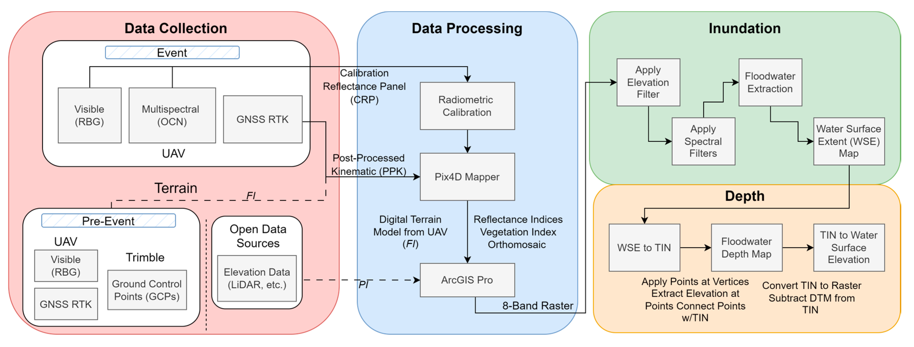
This paper introduces a novel, rapidly deployable UAV water surface detection method referred to as UAV–Floodwater Inundation and Depth Mapper (FIDM). The methodology is summarized in Figure 1. The three major components are (1) aerial data collection, (2) data processing, and (3) floodwater inundation (water surface extent) mapping and depth mapping. UAV-FIDM is carried out for two modes, namely a partial (LiDAR-derived) integration (PI) and full (UAV-DEM-derived) integration (FI). The PI makes use of any existing elevation data from publicly available sources, such as from the US Geological Society (USGS), while the FI generates elevation from data obtained by the UAV and further utilizes them in deriving the final surface extent and depth products.
2.1. Study Area
The study area is located in the Town of Elkin, Surry County, North Carolina, USA (Figure 2). The Yadkin River flows just south of the Historic Elkin Downtown District. With headwaters originating in the Blue Ridge Mountain foothills, it forms the northernmost part of the Pee Dee drainage basin. The Yadkin River is regulated upstream of the project site at the W. Kerr Scott Dam and Reservoir in Wilkesboro, North Carolina. The region is characterized by forests of mixed hardwoods, including hickory, sycamore, and poplar. The project site was selected due to ease-of-access, combined with the high likelihood of riverine flooding induced by Hurricane Zeta. The study area consists of the Downtown District at U.S. 21 Business and the Yadkin River and includes six road closures due to flooding at U.S. 21 Business, Commerce St., Elk St., Standard St., and Yadkin St. The total project area is approximately 0.39 km2 (100 acres) and is bounded by WGS 84 coordinates of 36°14′40″ N, 80°51′15″ W (northwest), 36°14′40″ N, 80°50′45″ W (northeast), 36°14′15″ N, 80°50′45″ W (southeast), and 36°14′15″ N, 80°51′15″ W.
2.2. UAV Platform and Sensors
The UAV used in this study is a customized DJI Phantom 4 Pro quadcopter (P4P). The P4P is equipped with a 1-inch, 20-Megapixel CMOS camera. The lens is 8 mm × 24 mm with a field of view (FOV) of 84°. The image size is 5472 × 3648 pixels with output in JPEG and DNG format. A GNSS receiver (rover) is linked to the camera’s shutter signal to record precise time marks and coordinates for every photo taken. A second RTK GNSS receiver (base) is installed on a survey monument and records a fixed position for the duration of the flight. The GPS measurements from the base are used to apply corrections to the rover, using a Post-Processed Kinematic (PPK) workflow, providing survey-grade positioning. The sensor dataset associated with the UAV’s primary camera is herein referred to as RGB.
The UAV is also equipped with a Mapir Survey 3W (3W) multispectral sensor, with an external GPS used for geotagging. The sensor is a Bayer color filter array with 12 Megapixels and an image size of 4000 × 3000 pixels in TIFF format. The 3W records on three channels, namely orange, cyan, and near-infrared, with spectral peaks at 490 nm, 615 nm, and 808 nm, respectively. The 3W reflectance values are radiometrically calibrated to compensate for day-to-day variations in ambient light, using a calibrated reflectance panel (CRP). The CRP contains four diffuse scattering panels in black, dark gray, light gray, and white that are lab-measured for reflectance between 350 nm and 1100 nm. A unique reflectance profile is established for each panel, which converts an established wavelength to reflectance percent. An image of the CRP is captured on the 3W immediately before and after each flight. The CRP images are then used in post-processing to convert each pixel from bit depth to reflectance percent, using the panel profiles and metadata (gain/bias settings for each channel), allowing for a reflectance calibration of less than 1.0% error in most cases (MAPIR CAMERA, San Diego, CA, USA). The sensor dataset associated with the 3W is herein referred to as OCN.
2.3. Flooding Event and Aerial Data Collection
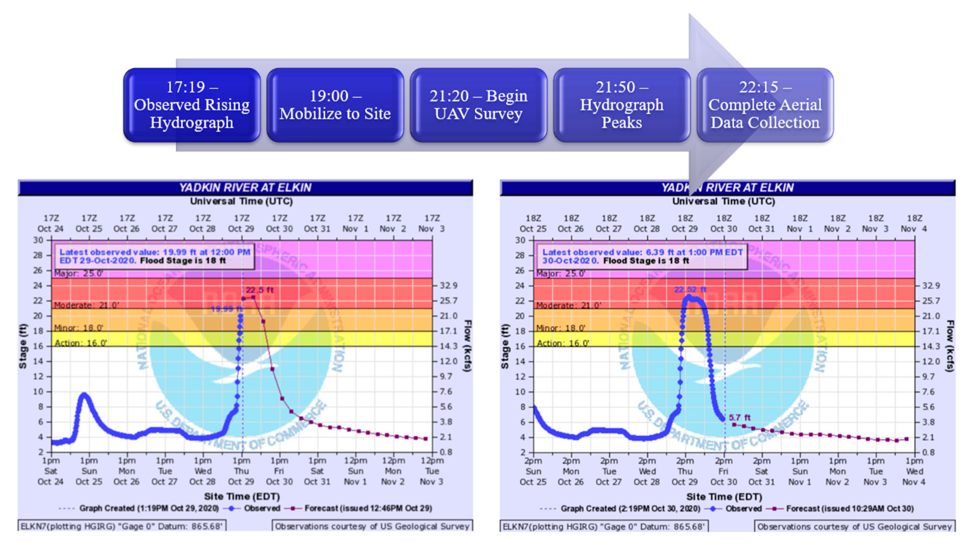
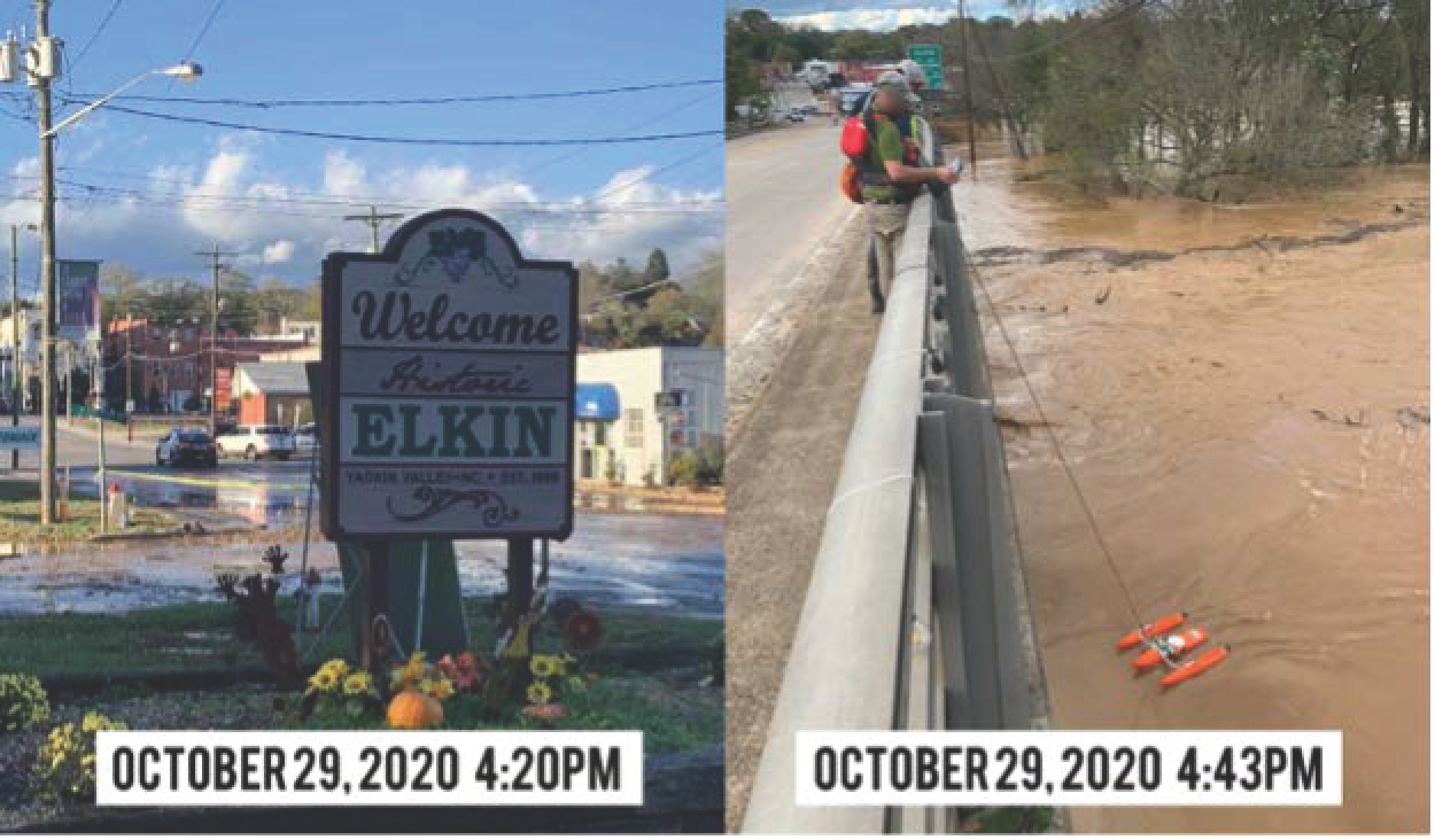
More than a dozen locations throughout the Carolinas during the 2020 hurricane season were monitored by the UAV data collection team, using the National Weather Service (NWS) River Forecast Center and NWS precipitation products. The Hurricane Zeta event and study area were finalized based on accessibility and data availability. The finalized aerial survey location was selected based on real-time correspondence with first responders of the Town of Elkin Police Department during the event. USGS gauge 02112250, located at 36°14′27.73″ N, 80°50′56.86″ W, was consulted to estimate the flood stage and time-to-peak (Figure 3). The team arrived on-site during the rising limb of the hydrograph (Figure 3) on 29 October 2020, at 20:00 UTC.
Prior to mobilizing to the site, two flight plans were created to automate UAV data collection to ensure optimal coverage and to minimize human error, using a flight-planning app created by Litchi. The flying height was set to 118.9 m above ground level (AGL) or 395.0 m above mean sea level (AMSL). The forward speed was set to 23.4 kph. The percent forward and side overlap were both set to 80%. The exposure time was set to 300/s to avoid image blurring for both the RGB and OCN datasets. Aerial data collection was conducted over two 25-min flights. The first flight commenced at 21:20 UTC and concluded at 21:45 UTC. The second flight commenced at 21:50 UTC and concluded at 22:15 UTC. Representatives from the United States Geological Survey (USGS) were also on-site monitoring the velocity, peak flow, and stage (Figure 4). The UAV team coordinated with the USGS to determine an approximate time-to-peak of 21:50 UTC. Using the recorded conditions at the gauge and field-verified measurements from the USGS, it was confirmed that the peak stage elevation of 270.72 m (888.20 ft) was concurrent with the time of the aerial data collection. The resulting nominal ground sample distance (GSD) was 3.3 cm for RGB and 5.5 cm for OCN.
On 29 November 2022, the same UAV and sensor configuration were deployed using the same flight plans. This second aerial dataset was used to generate a digital elevation model (DEM) during non-flooding conditions, as well as to provide a post-event multispectral dataset. It should be noted that the supporting dataset should ideally be collected prior to the flooding event. However, capturing data after the event produces identical results but has the disadvantage of not being able to provide near-real-time information. The DEM data are further utilized in the FI model for the final results.
2.4. Ground Truthing Data
Two sets of ground-truthing data were collected for the study. The first set was collected during the flooding event on 29 October 2020 and consisted of ten geolocated floodwater depth measurements. A Trimble R10 RTK GNSS system and TSC5 data collector (Trimble, Sunnyvale, CA, USA) were used to collect position and elevation data for two ground-truthing datasets. For this process, Trimble Access was used to create a general survey in NAD 1983 State Plane North Carolina FIPS 3200 coordinates, and the RTKNet was used to establish a VRS session. The floodwater depth measurements were taken using a fiberglass grade rod after the second and final UAV flight. After depth was recorded, the position was recorded using the Trimble. An occupation time of 90 s was chosen to achieve the desired accuracy (approx. 1 cm horizontal and 3 cm vertical). The measurements were uniformly spaced within the downtown district, primarily in flooded roadways. These depth measurements were used for model validation and are discussed in Section 4.3.
For the second set, twelve Ground Control Points (GCPs) were collected on 29 November 2020. The 29 October 2020 dataset was initially used to identify potential GCP locations by identifying objects or structures in the true-color orthomosaic that were present during flooding conditions, such as roadway paint markings, cracks in the sidewalk, centers of manholes, etc. The potential GCPs were further identified in the field on November 29, and their position was recorded using the Trimble, with an occupation time of 180 s. All twelve GCP positions each recorded three different times throughout the day. The final positions of the GCPs were calculated as the average of the three measurements to achieve the desired accuracy of approx. 1 cm horizontal and ≤3 cm vertical. The GCPs were then used to composite the 29 October 2022 dataset for generating the final results. The GCPs were also used to generate a digital elevation model (DEM) for the 29 November 2020 dataset during “leaf-off” conditions. The data processing is discussed in the following section.
2.5. Data Processing
Two types of data were processed in this study. The first type was two-dimensional multispectral data, including orthomosaics (RGB and OCN), and the second was three-dimensional elevation data (DEM). Both types were processed with the software Pix4DMapper Ver 4.5.12. All images taken by the UAV were processed with a Structure-from-Motion (SfM) and multi-view stereo approach [43,44]. These approaches allow the geometric constraints of camera position, orientation, and GCPs to be solved simultaneously from many overlapping images through a photogrammetry workflow. Twelve steps were required to generate the orthomosaics and DEM:
- The RGB and OCN image datasets were acquired using a UAV platform on a gridded automated flight plan;
- GCPs were collected as Trimble survey points with an accuracy of ±1 cm horizontal and ±3 cm vertical;
- PPK processing was performed to provide RGB images with geotagged locations with an accuracy of ±5 cm;
- OCN images were preprocessed to provide reflectance calibration;
- RGB images were imported into Pix4DMapper, together with the information about acquisition locations (coordinates), including the roll, pitch, and yaw of the UAV platform. The information was used for the preliminary image orientation;
- “Matching” in Pix4D comprised three steps: First, a feature-detection algorithm was applied to detect features (or “key points”) on every image. The number of detected key points depends on the image resolution, image texture, and illumination. Second, matching key points were identified, and inconsistent matches were removed. Third, a bundle-adjustment algorithm was used to simultaneously solve the 3D geometry of the scene, the different camera positions, and the camera parameters (focal length, coordinates of the principal point and radial lens distortions). The output of this step was a sparse point cloud.
- The GCP coordinates were imported and manually identified on the images. The GCP coordinates were used to refine the camera calibration parameters and to re-optimize the geometry of the sparse point cloud.
- Multi-view stereo image-matching algorithms were applied to increase the density of the sparse point cloud into a dense point cloud.
- A digital surface model (DSM), which consists of a textured map, was derived from all images and applied to the polygon mesh that was used to create an orthomosaic.
- The DSM and orthomosaics for RGB and OCN were exported from Pix4DMapper into ArcGIS Pro.
- A digital elevation model (DEM) generated from the RGB point cloud and exported from Pix4DMapper into ArcGIS Pro. Alternatively, a DEM can be generated using LiDAR data for faster results. Both UAV-DEM-derived and LiDAR-derived results are explored in the following sections and are referred to as the full-integration (FI) mode and partial-integration (PI) mode, respectively.
- RGB, OCN, and DEM were combined into a single raster file in ArcGIS Pro for analysis.
2.5.1. Model Data
The extraction model utilizes an 8-band raster dataset composited from three datasets: (1) very high resolution imagery (RGB), (2) multispectral imagery (OCN), and (3) topographic data (DEM/LiDAR). The RGB and OCN cameras record data in JPEG and TIFF format, respectively. The values are converted to reflectance percent by dividing the pixel values by the bit depth of the image format. RGB data are in raster format with reflectance stored as 8-bit digital numbers (DNs) ranging from 0 to 255. The data are decomposed into separate bands for red, green, and blue. The RGB DNs are normalized to values ranging from 0.00 to 1.00 by dividing by 255:
OCN data are also in raster format, with reflectance stored as 16-bit DNs ranging from 0 to 65,535. The data are provided on separate bands for orange, cyan, and near-infrared (NIR). The OCN data are also normalized by dividing by 65,535:
NDVI is a unitless fraction given as the difference of reflectance between NIR and red, divided by the summation of NIR and red [45]. The authors theorized that the delineation of floodwater is enhanced in densely vegetated areas due to the low NDVI values of floodwater and high NDVI values of live green vegetation. In this study, orange was substituted for red to reduce the pixel noise associated with the high red reflectance of soil [46]. NDVI is given, then, as follows:
The required topographic data depend on whether the fully integrated (FI) or partially integrated (PI) model is employed. The FI model utilizes a DEM derived from photogrammetry (UAV-DEM-derived), while the PI model utilizes a DEM derived from the LiDAR (LiDAR-derived). Finally, RGB, OCN, NDVI, and DEM/LiDAR are composited into a single raster dataset with 8 bands by the proposed algorithm explained in the following section.
2.5.2. Water Surface Extent Algorithm
Inundation, or water surface extent (WSE) mapping, is performed using a two-step algorithm based on the 8-band orthomosaic. Step one is optional and is used for riverine floods in which the user defines an elevation above mean seal level (AMSL) which eliminates pixels above the estimated flood stage. This step should be skipped for flash floods in which inundation is highly localized and may be independent of river stage. In this study, the flooding of the Yadkin River at Elkin, North Carolina, was the result of flood routing as opposed to direct precipitation. All flooding, then, was the result of overbank flow, in which the floodwater depth was directly correlated with the river stage. As such, a maximum elevation corresponding to the peak stage of 270.72 m (888.20 ft) AMSL was utilized from the forecasted conditions at the local USGS gauge 02112250. Band-8 pixels corresponding to elevations above 270.72 m were automatically annotated as non-floodwater and eliminated prior to step two. It should be noted that the user must consider the hydraulic profile of the river when selecting an elevation threshold. For smaller study areas (up to 1 km2), using an elevation threshold corresponding to a local stream gage should suffice; however, for larger study areas (over 1 km2), the elevation threshold should not be used or must be defined by the maximum potential WSE (most upstream cross-section) for the study reach. For the full model and partial model, the DEM and LiDAR were used to determine the maximum elevation threshold, respectively.
In step two, the user defines a spectral profile to extract floodwater pixels from the remaining dataset. The spectral profile is constructed from two or more spectral reflectance curves by manually sampling pixel values for area(s) of interest, using a lasso drawing tool. In this study, visual inspection was used to identify major color variations within the flooded areas. This led to establishing four spectral reflectance curves, as shown in Figure 5, corresponding with (1) overbank flooding, (2) channel flooding, (3) overbank flooding covered in shadow, and (4) riverine flooding covered in shadow. Overbank flooding corresponds to inundation outside of the main channel banks. Overbank flooding appears in the model as sheet flow with a laminar surface. The flow is generally shallow (0–2 m deep), with little to no debris present. Channel flooding, on the other hand, appears in the model ranging from laminar to turbulent flow. Perturbations and debris are present throughout the floodwater surface. Both overbank and channel flooding appear in the true-color orthomosaic as reddish brown due to the iron-rich loamy soil typical of the region. The channel flooding is generally more consistent with higher values of red, green, and blue. Overbank flooding has higher values in orange, cyan, and near-infrared, likely due to the relatively shallow flow, in which grass, asphalt, and concrete are sometimes partially exposed. The shadows have the effect of uniformly lowering the brightness values across the spectrum for both overbank and channel flooding. NDVI values are invariably low across all four curves due to the lack of photosynthetic material in the water. The minimum and maximum pixel values extracted for each band are also presented in the box and whisker plots for Figure 5. The complete spectral profile is provided in Table 1 in the column “Extraction Range”. It should be noted that the distribution of data is less for OCN due to the narrow-filtered bands of the multispectral sensors.
After the maximum elevation and spectral profile are defined, the water extraction model works by masking or eliminating pixels outside the specified ranges, as specified in Table 1, chronologically. First, DEM/LiDAR values greater than 270.72 m (888.20 ft) AMSL are eliminated, followed by the pixels with NDVI less than 0.2 and within the extraction range for each band. Any pixels not eliminated are automatically annotated as floodwater pixels. The model output includes a binary raster file, with 0 representing non-floodwater pixels and 1 representing floodwater pixels. The result is a water surface extent (WSE), or inundation map. It should be noted that, while the model will extract floodwater pixels, it will not extract non-floodwater pixels unless a spectral reflectance curve is generated specific to non-floodwater. For example, a wet detention pond, which is generally free from sediment, will have a significantly different profile from sediment-rich floodwaters and will not be extracted. The output layers are shown in Figure 6.
2.5.3. Water Depth Algorithm
A water depth map is generated from the WSE (inundation) map and a bare-earth topographic dataset (DEM/LiDAR), using a 6-step process, which is illustrated by Figure 7.
Step (1): Non-floodwater pixels are removed from the raster dataset by setting 0 values to null.
Step (2): The raster is converted into a feature layer; this procedure generates polygons for contiguous patches of floodwater, including individual floodwater pixels. Polygons with an area below a user-defined threshold are removed. In this study, a minimum area of 3 m2 was used to remove smaller patches.
Step (3): Points are generated at a user-defined interval along the edges of the polygons or the edge of the floodwater extent where depth is assumed to be 0.00 m. For this study, points were generated every 3 m. Elevation data are extracted from the DEM at each point, representing the floodwater elevation at that point.
Step (4): Points are connected to form a triangulated irregular network (TIN), using linear interpolation. Each triangle forms a plane representing the floodwater elevation, capturing variations in the water surface profile.
Step (5): The TIN is converted to a raster format, depicting a floodwater elevation map.
Step (6): Finally, the DEM is subtracted from the floodwater elevation map to provide a floodwater depth map. Figure 8 illustrates the TIN-to-depth process for a selected portion of the model.
2.6. Model Output
The final output for both the FI and PI models consists of a single raster file containing the modeled inundation and depth with a resolution of 3.3 cm, and the output results summarized in Table 2. For the FI model, the input raster was reduced from 396,158,137 total pixels to 101,462,379 floodwater pixels (25.6%); thus, 74.4% of the total pixels were eliminated. For the PI model, the input raster was reduced from 396,158,137 total pixels to 129,453,581 floodwater pixels (32.7%); thus, 67.3% of the total pixels were eliminated. For both models, inundation is represented by the spatial distribution of the remaining pixels, while depth is stored as the pixel value. While the models have no inherent limitations for inundation mapping, depth calculations are generally limited to floodwaters outside of the main channel due to the inability of photogrammetry and most LiDAR devices to penetrate water, with the exception of green LiDAR [47]. The bathymetric surface, therefore, cannot be mapped, and the area within the wetted width of the channel is clipped prior to analysis. After removal, the FI model depth ranges from 0.00 m to 9.14 m, with a mean depth of 2.25 m. The PI model depth ranges from 0.00 m to 5.76 m, with a mean depth of 1.25 m. It should be noted that the mean depth of the PI model is significantly lower due to a higher commission error, which is discussed in Section 3.2.
3. Validation and Results
3.1. Inundation Validation
The accuracy of the inundation models was assessed using human annotation for validation [48]. This process is time-consuming and labor-intensive and requires the user to manually annotate or “flag” pixels by visually inspecting the true-color orthomosaic. Multispectral mosaics, therefore, were not included in the visual inspection, e.g., OCN and NDVI. The criteria utilized for the identification of floodwater pixels are divided into two categories. For the riverine category, the water surface within the main channel, which is known to be flooded by reference to a stream gauge, is visually scanned from the center line and outward to where land or built structures become visible. For overbank flooding, pixels corresponding with ponded water, with colors consistent with riverine flooding, are also flagged. Recent aerial and satellite photos under non-flooding conditions are also visually compared to reduce human error and prevent the flagging of permanent water features, such as retention ponds. For this study, the floodwater was sediment-rich and opaque, leading to a distinct color profile for easy detection. For efficiency, a patch-wise approach was utilized by annotating pixels coinciding with the edge of the floodwater, as opposed to a pixel-wise approach, which would require over one hundred million annotations [49]. Once the edges were identified, the floodwaters were bounded using non-overlapping polygons. The patch-wise procedure required over 100,000 annotations and took over 30 h to complete. Polygons were then converted to raster format; resampled; and adjusted to match the extent, resolution, and cell alignment of the inundation modeling results. The validation raster is herein referred to as Validation, and the modeled inundation rasters are referred to as PredictedUAV (FI model) and PredictedLiDAR (PI model).
In order to evaluate the accuracy of the UAV-DEM-derived inundation model, two sets of data are defined. The first set is Validation (V) and contains 108,977,736 pixels. The second set is PredictedUAV (PUAV) and contains 101,462,379 pixels. The first relation, V ∩ PUAV, is the intersection of Validation and PredictedUAV in which the model correctly extracted floodwater pixels. V ∩ PUAV contains 96,800,615 pixels, indicating that the inundation model successfully extracted 88.8% of V. The second relation is the set difference PUAV\V containing 4,662,185 pixels. PUAV\V indicates that misidentifications, or commission errors, make up 4.59% of PUAV. The third relation is the set difference V\PUAV containing 12,177,322 pixels. V\PUAV indicates that the inundation model failed to extract 11.2% of V, representing an omission error. A total of 10,329,127 pixels in V\PUAV, or 84.8%, are located in areas with dense tree cover. This suggests that the model’s performance is poor when the floodwater is obscured by tall vegetation. When excluding these areas from the analysis, the inundation model only fails to extract 1.9% of V.
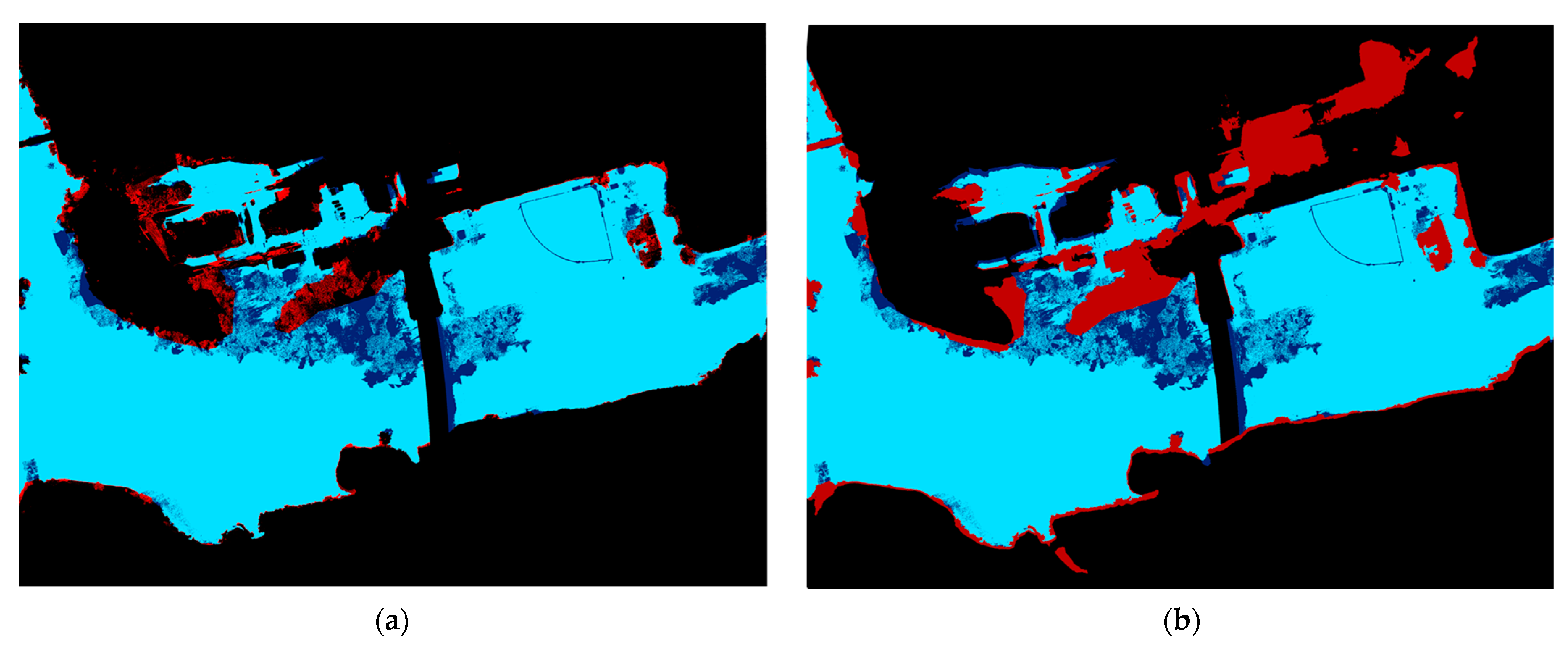
The accuracy evaluation was repeated for the PI model, referred to as PredictedLiDAR (PLiDAR), which contains 127,942,429 pixels. V ∩ PLiDAR contains 95,728,050 pixels, indicating that the PI model successfully extracted 87.8% of V. The second relation, PLiDAR\V, contains 20,263,948 pixels, indicating that 15.8% of PLiDAR is a commission error. The third relation, V\PLiDAR, contains 24,728,013 pixels, indicating that the partial model failed to extract 22.7% of V, representing an omission error. When omitting areas of dense tree cover, the LiDAR-derived inundation model fails to extract 14.6% of V. Table 3 provides a summary of the FI and PI model inundation analyses. The floodwater inundation maps, showing the spatial distribution of accuracy and omission and commission errors, are shown in Figure 9. There are several potential reasons for the higher commission and omission errors in the PI model compared to the FI model, and these are discussed in more detail in Section 4.1.
3.2. Depth Validation
The accuracy of the depth model was assessed by measuring the depth at ten locations, using a 7.62 m (25-foot) fiberglass grade rod, accurate to 3 cm. The measurements were taken immediately after the second and final UAV flight on 29 October 2020. The measurements were uniformly spaced within the Downtown District, primarily on impacted roadways. Measurement locations were limited to areas that could be safely reached on foot. Due to safety concerns, this is not the preferred method, and we recommend that depth validation be conducted from a vessel for future studies. Measurements ranged from 3.1 cm to 39.6 cm in depth. Figure 10 shows the spatial distribution of measurement locations. Table 4 shows the depth predicted by the FI model, the depth predicted by the PI model, the actual depth as measured on the grade rod, and the percent difference between Measured and Predicted. The total differences in depth and percent for the FI model range from −3.1 cm to 6.1 cm, with an average difference of 1.8 cm and with an average percent difference of 13%, respectively. The total differences in depth and percent for the PI model range from −13.2 cm to 58.0 cm, with an average difference of 4.8 cm and with an average percent difference of 34%, respectively.
To further quantify the accuracy of the UAV-DEM- and LiDAR-derived depth models, the root mean square error (RMSE) was calculated using Equation (8):
where is the depth (cm) extracted from the UAV-DEM and LiDAR-DEM at each measured location; is the measured ground truthing depth; and N is the total number of comparisons, which is ten (10) for this study. The UAV-DEM-derived depth model outperformed the LiDAR-derived depth model (RMSE of 3.6 cm and 43.0 cm, respectively).
3.3. Land Type Classification
In order for the floodwater pixels to be extracted by the floodwater inundation model, the floodwater must be visible to the sensors on the UAV platform. The authors hypothesized that model performance is adversely impacted by obstructions to the land/water surface, such as trees, buildings, and other natural and artificial structures. The presence of obstructions increases spectral heterogeneity and decreases the separability of floodwater pixels from background noise. To evaluate this hypothesis, a 2020 land-cover raster with 10 m resolution was obtained from the European Space Agency WorldCover 2020 Database [28]. Three relation set percentages, namely omission error, commission error, and percent correct, can be calculated using pixel counts and are evaluated per land-cover type:
Six land-cover types were observed in the study area, and the results are summarized in Table 5. In terms of correct %, the UAV-DEM-derived inundation model (FI) performed best for Cropland (95%), followed by Grassland (84%), Permanent Water Bodies (78%), Built-Up (70%), Bare/Sparse Vegetation (60%) and lastly Tree Cover (55%). In terms of omission %, the FI model has the most difficulty identifying floodwater in Tree Cover (34%), followed by Bare/Sparse Vegetation (26%), Built-Up (17%), Permanent Water Bodies (15%), Grassland (10%), and lastly Cropland (3%). Commission % is less dispersed for the FI inundation model, with the highest frequency occurring in Bare/Sparse Vegetation (14%), followed by Built-Up (13%), Tree Cover (10%), Permanent Water Bodies (7%), Grassland (6%), and lastly Cropland (2%).
The correct % was calculated for the LiDAR-DEM-derived inundation model (PI) model for the six land-cover types. The performance was best for Water Bodies (80%), followed by Grassland (74%), Built-Up (54%), Tree Cover (51%), Bare/Sparse Vegetation (46%), and lastly Cropland (25%). The FI inundation model performed better for Grassland, Built-Up, Bare/Sparse Vegetation, and Cropland due to the absence of trees combined with the higher resolution and accuracy of the elevation data. In terms of the omission error, the LiDAR-derived inundation (PI) model has the most difficulty identifying floodwater in Cropland (58%), followed by Tree Cover (35%), Bare/Sparse Vegetation (18%), Permanent Water Bodies (14%), Built-Up (5%), and lastly Grassland (2%). While the FI model performed the best for Cropland, the PI model performed the worst for Cropland. The visual inspection reveals significant differences in elevation between the UAV-DEM and LiDAR-DEM elevations in the Cropland area; however, it is unclear why the discrepancies exist. It should be pointed out, however, that Cropland only accounts for 4.3% of the land-cover dataset and, hence, a smaller sample size of pixels. The commission error is highest for Built-Up (41%), followed by Bare/Sparse Vegetation (36%), Grassland (24%), Cropland (17%), Tree Cover (14%), and lastly Permanent Water Bodies (6%).
4. Discussion
4.1. Full versus Partial Model Discussion
The validation results presented in Section 3.1 indicate that the UAV-DEM-derived inundation model (FI model) outperformed the LiDAR-derived inundation model (PI model) with respect to the commission error and omission error. The FI model successfully extracted 88.8% of the validation pixels, with a commission error of 4.59% and an omission error of 11.2%. The PI model performed slightly worse, with a successful extraction rate of 87.8%, a commission error of 15.84%, and an omission error of 22.69%. It should be emphasized that the only difference in model input between the FI and PI models is the elevation raster dataset. It should be emphasized that using the PI model will not necessarily lead to a decrease in performance; high-resolution terrain models are already available for many flood-prone areas, and the PI model may be a better alternative depending on the quality of the topographic data.
Our examination of the PI model revealed an extensive commission error in the northeastern quadrant. This portion of the LiDAR-DEM is relatively flat, with the majority of the pixel values falling within the flood threshold (≤270.72 m), as defined in Table 1. Conversely, this same area in the UAV-DEM is slightly above the flood threshold (>270.72 m), preventing these pixels from being flagged as “floodwater”. Upon examination of Figure 9, the variability of omission error is less pronounced. The higher omission error of the PI model is likely related to the coarser resolution of the LiDAR-DEM. The two methods tend to miss pixels within the same regions; however, the density of omissions is greater in these regions for the PI model. It is hypothesized that the higher-resolution UAV-DEM captures more detail in the digital surface, including small depressions for flood storage. It is possible that these smaller depression areas are flattened or smoothed out during the preprocessing of the LiDAR-DEM.
There are several potential mitigation strategies for improving model performance in areas with dense vegetation and shadows. The greatest source of error associated with vegetation occurs within patches of tree cover over floodwater. UAV-FIDM does not possess a decision structure allowing assumptions beyond the floodwater flagging mechanisms, i.e., elevation and spectral profile. This shortcoming could be improved by introducing a new spectral profile for trees. Any contiguous patch of trees surrounded by floodwater pixels on all sides would then be assumed to be inundated also. The primary issue with shadows is that they uniformly lower the brightness values across the spectrum, making it difficult to discern floodwater pixels covered in shadow from other dark features. One potential method for addressing this issue is to include a third sensor on the UAV platform consisting of a radiometrically calibrated thermal camera. In addition to the visible and near-infrared color profile, a thermal camera could be used to isolate floodwater from the background by developing a longwave infrared profile. It is assumed that the floodwater temperature would remain relatively constant across the dataset, with only minor variations in shadows. This additional layer could be ingested into the existing workflow, as shown in Figure 6, without major changes to the UAV-FIDM methodology. Both of these mitigation strategies will be explored in future work.
4.2. Land-Type Classification Discussion
The land-type classification has a considerable impact on the performance of the inundation models. The results indicate that the FI and PI models performed best for cropland and grassland, while tree cover posed the most significant challenge, with an omission error of 34% for the FI model. This is consistent with the hypothesis that dense and/or tall vegetation blocks the view of the sensors, concealing the spectral profiles associated with floodwater underneath. The PI model was slightly better at extracting floodwater for Water Bodies due to the enhanced ability of LiDAR to penetrate the dense tree canopy along the edge of the river, where vegetation is widespread.
A second cause of omission error, associated with vegetation, is related to the generation of the UAV-DEM using photogrammetry. The photogrammetry software, Pix4DMapper, classifies the densified point cloud by using machine-learning techniques based on geometry and color information [29]. Some vegetation is difficult to classify and remove from the DEM, especially when the vegetation is dense and the ground is not visible. This may have the effect of artificially raising the elevation of what is assumed to be ground for densely vegetated areas within the model. These artificially high elevations will be erroneously filtered from the floodwater pixel extraction procedure if the elevations are above the user-defined threshold, leading to omission error.
By visual inspection, we can see that a significant portion of the commission error is associated with shadows. Shadows are most prevalent for Bare/Sparse Vegetation, Built-Up, and Tree Cover due to the heights of buildings, trees, and tall vegetation. For these shadowed regions, the spectral profiles are similar to (1) overbank flooding covered in shadow and (2) riverine flooding covered in shadow. Here, the reflectance values across the spectral profiles are exceedingly low, to the degree that the model is unable to resolve the difference between floodwater and noise in some shadowy areas. The shadows are a function of the solar angle of incidence corresponding with the time of day the UAV flights were conducted, occurring 60–100 min prior to official sunset. Because this methodology was developed to monitor real flooding events, the time of data collection is dependent on the peak discharge; it is therefore not possible to avoid shadows from entering the dataset in order to maintain the flexibility of the method. Future studies will be dedicated to identifying floodwater pixels in shadowed regions to improve the model’s accuracy.
4.3. Depth Results Discussion
For the PI model, the model was developed using the same layers, filter thresholds, and extraction method, with the exception that elevation is provided by USGS LiDAR data instead of UAV-DEM. Using LiDAR is necessary to estimate depth when a pre/post-elevation dataset is not available for the study area, which increases the applicability of the model. However, the model’s performance may be diminished depending on the availability, quality, and accuracy of the LiDAR data. The average difference in depth for the FI model was 1.8 cm, with an average percent difference of 13%. For the PI model, the average difference in depth was 4.8 cm, with an average percent difference of 34%. The better performance of the FI model may be attributed to the higher resolution and accuracy of the UAV-DEM due to a higher spatial density of ground control points and the timeliness of the data coinciding with the actual flooding event in 2020. The UAV-DEM was generated from a point cloud consisting of 28 points per meter. The LiDAR-DEM was derived using a linear aerial sensor and collected at 2 points per meter in 2014 [27]. It is possible that the topography changed during the intervening period between 2014 and 2020, either by natural processes, such as erosion and settling, or by manmade processes, such as land development, compaction, and grading. The temporal relevancy of the LiDAR-DEM can therefore have significant implications for the accuracy of the PI model and must be considered early on in the planning stages of near-real-time flood mapping efforts.
For this particular study, the accuracy of the inundation model was sufficiently improved so as to justify using UAV-generated DEM for elevation. This does require a pre- or post-event dataset to process flood inundation and pre-event flight specifically for near-real-time application. Producing a survey-grade UAV-DEM requires the collection of ground-truthing data for quality assurance. This requires planning, additional resources, and a desire to study a particular watchpoint. In many cases, however, the objective of near-real-time inundation and depth estimation is to provide crucial information to first responders wherever floods may happen. This often precludes the option of obtaining data in advance due to limited resources, budgets, and uncertainty where flooding may occur. In these instances, the inundation model still performs reasonably well with LiDAR and may even outperform the FI model depending on the topographic data quality. Further research will be required to compare the two models over different regions to quantify the potential trade-offs and benefits.
It is noted that a well-equipped and robust computational setup is instrumental in effectively deploying our algorithm for the generation of near-real-time flood inundation maps across expansive geographic scales. Nevertheless, it is important to acknowledge the practical constraints when applying this method in regions experiencing widespread flooding, such as those witnessed in Pakistan [50] or South Africa [51]. The potential challenges may arise, particularly in regions where data infrastructure might be inadequate or access to high-performance computing resources is limited. It is further noted that there are obvious challenges with respect to collecting the data. This requires not only access to UAVs equipped with multispectral sensors but also “boots-on-the-ground” operators with the ability to mobilize to critical watch points. Covering widespread flooding may require the coordination of dozens of operators given the limited swath provided by UAVs of only a few kilometers.
4.4. Other DEM-Derived Floodwater Depth Mapping Methods
Depth is an essential piece of information for first responders and post-event mitigation assessment. As an available tool for rapid surface water mapping, DEM-derived methods can provide an approximate depth during or after a flood event that can be validated by satellite images. The Floodwater Depth Estimation Tool (FwDET) has been proposed for rapid and large-scale floodwater depth calculation, using solely a flood extent layer (survey- or remote-sensing-derived) and a DEM [52].
As another point of comparison, we used this new cloud-derived GIS tool by inputting the UAV-DEM and LiDAR-DEM data into FwDET. Figure 11 shows the floodwater depth maps generated using (a) FI, (b) PI, (c) FwDET with UAV-derived DEM, and (d) FwDET with LiDAR-derived DEM. The blue-color ramp represents the estimated depth at each pixel. The red line represents the validation (extent) layer. When using the UAV-derived and LiDAR-derived DEMs as the base of the FwDET model, the resulting flood maps display several gaps along the channel and surrounding floodplains. This phenomenon has been identified and discussed in similar studies [16]. The gaps appear to be areas in which FwDET falsely identifies pixels as edges of the floodwater. The “edges” are flagged as zero water depth and tend to propagate outwards from individual pixels, failing to identify floodwater for large portions of the modeling domain. Another key limitation of FwDET is the appearance of “linear stripes along the flooded domain” in which “unrealistic differences in elevation between adjacent boundary grid-cells” cause sharp transitions, resulting in unrealistic visual representations. Both of these tendencies were prevalent when uploading the UAV-DEM and validation layer into the online GIS environment. It is evident that the edges and stripes can lead to large differences in the actual versus predicted values for shallow flood depths, and this may be problematic for urban flooding, where shallow flooding can have significant consequences for public safety.
In this investigation, the confluence of multiple remote-sensing data sources, specifically UAV-DEM and LIDAR-DEM, was employed. Leveraging these resources through a machine-learning approach enables the extraction of pertinent insights. The outputs generated serve as valuable tools for mapping flood inundation [53,54,55] and monitoring regions experiencing significant hydrological changes [56]. Machine-learning techniques also offer promising solutions to complex scenarios in which traditional methodologies may not be as effective. For example, Xu et al. [57] presented and discussed the potential of XGBoost and other similar algorithms in enhancing the efficacy in modeling shallow flood depths, a significant concern in urban environments. Sanders et al. [58] also presented the XGBoost in support of forecasting flood stages in the Flood Alert System (FAS). Tamiru et al. [54] found that integrating machine learning with HEC-RAS improved the accuracy of flood inundation mapping in the Baro River Basin, Ethiopia. Karim et al. [53] reviewed the literature on machine-learning and deep-learning applications for flood modeling and found that deep-learning models produce better accuracy compared to traditional approaches.
Table 6 shows the actual depth measured in the field; the predicted depth by FwDET, using the UAV-DEM (FwDET + UAV-DEM); and the predicted depth by FwDET, using LiDAR (FwDET + LiDAR). The FwDET using the UAV-DEM produces an average difference of −8.1 cm (standard deviation of 14.9 cm) and absolute percent difference of 106%, and the FwDET using LiDAR produces an average difference of +2.8 cm (standard deviation of 25.1 cm) and absolute percent difference of 109%. Compared to both the FwDETs’ results, the FI and PI show closer estimations at the measured locations, with the FI achieving the highest accuracy, i.e., 1.8 cm, as the average difference. In future studies, a portable unmanned catamaran platform capable of producing detailed hydrographic surveys will be used for depth validation, offering greater density and continuity of bathymetric data, while providing data in hard-to-reach or unsafe locations. This will help provide valuable insight into the accuracy of each method.
Recognizing that the scale of flood waves and the spatial extent of flooded areas have increased in recent years, one potential application for UAV-FIDM is the monitoring of flood waves. Turlej et al. [59] analyzed the extent and effects caused by flood waves on a national scale in Central Europe, using MODIS satellite images for delineation of flooded areas. They noted difficulty in acquiring sufficient images during flood development due to cloud cover, as well as coarse data which were unable to resolve flood pools in tributaries and upper sections of rivers. UAV-FIDM is potentially well-suited to supplement these studies by providing high-resolution data to produce detailed maps of flood extents, river channels, and topographic features. This level of detail enhances the precision of flood modeling and supports better decision-making in flood management. There are several possibilities for creating a network of qualified UAV pilots to support flood risk management on a county, state, or national scale [60,61]. The UAV-FIDM methodology may be incorporated into these national efforts by coordinating on-site UAV deployment combined with cloud-based computation, such as Amazon Web Services, to deliver results over significantly larger areas.
5. Conclusions
This study introduces a novel method, referred to as UAV-FIDM, for near-real-time inundation extent and depth mapping for flooded events, using an inexpensive, UAV-based multispectral remote-sensing platform. The study proposes two methods including a fully integrated (FI) model that utilizes the UAV sensors to create an elevation dataset versus a partially integrated (PI) model that leverages existing datasets such publicly available LiDAR. The trade-offs between the full and partial models were evaluated. The advantages of the FI model include temporal currency of the pre-event elevation dataset and greater accuracy with respect to inundation and depth mapping due to higher spatial resolution and increased density of ground control points. The main disadvantage of the full model is that, in order to operate it in near-real-time, a pre-event elevation dataset must be collected. This requires additional sensors, planning, and foresight to collect the requisite level of data within the study area before flooding occurs. The PI model, on the other hand, provides greater flexibility and applicability because it does not require the user to anticipate where flooding may occur provided that the elevation data are readily available for the flooded area. The disadvantage is that pre-existing elevation data sources may not be available or recent and may be of lower quality than UAV-derived elevation datasets. The implications of such trade-offs are provided for the consideration of researchers.
UAV-FIDM is designed to be applicable for urban environments under a wide range of atmospheric conditions, including light precipitation and winds up to 50 km/h. It has an advantage over traditional remote-sensing platforms because it can fly beneath cloud cover while providing highly detailed maps for areas up to 3 square kilometers with a resolution of 6 cm or better. The limitations of UAV-FIDM include a processing time of up to 6 h, a relatively small coverage area, and the requirement of an operator to be on-site during the flooding event. The performance varies with land use, with the best performance being associated with lightly vegetated areas, including cropland and grassland, and the worst performance being associated with heavily wooded areas, such as forests or dense scrublands. This work reveals the shortcomings of UAV-FIDM in areas of dense vegetation or shadows and puts forth multiple suggestions to mitigate these issues.
Overall, UAV-FIDM is suggested as a supportive tool for mapping flood extent and depth in various fields, including hydrology and water management. Future studies will include the use of a thermal sensor to overcome the challenges presented by shadows and mitigate the errors associated with dense vegetation by adding a decision-making structure. Additionally, a detailed hydrographic survey will be used for validating the depth model. The methodology was tested and applied during an actual flooding event for Hurricane Zeta during the 2020 Atlantic hurricane season and shows that the UAV platform is capable of predicting inundation with a reasonably low total error of 15.8% and yields flooding depth estimates accurate enough to be actionable by decision-makers and first responders.
Author Contributions
Conceptualization, Z.N.F., D.L. and K.J.W.; methodology, D.L. and K.J.W.; software, D.L. and K.J.W.; validation, D.L. and K.J.W.; formal analysis, Z.N.F., D.L, W.L. and K.J.W.; investigation, Z.N.F., D.L. and K.J.W.; resources, Z.N.F.; data curation, W.L. and K.J.W.; writing—original draft preparation, D.L. and K.J.W.; writing—review and editing, K.J.W., D.L. and Z.N.F.; visualization, W.L., D.L. and K.J.W.; supervision, Z.N.F. and D.L.; project administration, Z.N.F. and D.L.; funding acquisition, Z.N.F. All authors have read and agreed to the published version of the manuscript.
Funding
This research was funded by the National Science Foundation, grant numbers 1832065 and 1940163.
Data Availability Statement
The data presented in this study are available on request from the corresponding author, Z.N.F., upon reasonable request.
Acknowledgments
This research is the culmination of a multi-disciplinary and multi-institutional collaboration between researchers and professionals that the authors would like to acknowledge. We would like to thank our collaborators—Qunying Huang, Daniel Wright, and Song Gao at the University of Wisconsin at Madison and Yi Qiang at the University of South Florida for the technical support on monitoring the hurricane and finalizing the mobilization plan. The authors would also like to thank Captain Jack Gonzalez of the Harrisburg Fire Department, the U.S. Army Corps of Engineers (USACE) Kitty Hawk Research Facility Center, U.S. Geological Survey (USGS) staff and field crew, and members of the Town of Elkin fire department, police department and first responders for their assistance in the planning and execution of this research. Lastly, we would like to thank three anonymous reviewers and the editor for their insightful suggestions for the paper.
Conflicts of Interest
The authors declare no conflict of interest.
References
- Li, Z.; Gao, S.; Chen, M.; Gourley, J.J.; Hong, Y. Spatiotemporal Characteristics of US Floods: Current Status and Forecast under a Future Warmer Climate. Earths Future 2022, 10, e2022EF002700. [Google Scholar] [CrossRef]
- Tabari, H. Climate Change Impact on Flood and Extreme Precipitation Increases with Water Availability. Sci. Rep. 2020, 10, 13768. [Google Scholar] [CrossRef]
- Hirabayashi, Y.; Mahendran, R.; Koirala, S.; Konoshima, L.; Yamazaki, D.; Watanabe, S.; Kim, H.; Kanae, S. Global Flood Risk under Climate Change. Nat. Clim. Chang. 2013, 3, 816–821. [Google Scholar] [CrossRef]
- Kirezci, E.; Young, I.R.; Ranasinghe, R.; Muis, S.; Nicholls, R.J.; Lincke, D.; Hinkel, J. Projections of Global-Scale Extreme Sea Levels and Resulting Episodic Coastal Flooding over the 21st Century. Sci. Rep. 2020, 10, 11629. [Google Scholar] [CrossRef]
- Floods|World Meteorological Organization. Available online: https://public.wmo.int/en/our-mandate/water/floods (accessed on 15 June 2023).
- Chetpattananondh, K.; Tapoanoi, T.; Phukpattaranont, P.; Jindapetch, N. A Self-Calibration Water Level Measurement Using an Interdigital Capacitive Sensor. Sens. Actuators Phys. 2014, 209, 175–182. [Google Scholar] [CrossRef]
- Marin-Perez, R.; García-Pintado, J.; Gómez, A.S. A Real-Time Measurement System for Long-Life Flood Monitoring and Warning Applications. Sensors 2012, 12, 4213–4236. [Google Scholar] [CrossRef] [PubMed]
- De Camargo, E.T.; Spanhol, F.A.; Slongo, J.S.; Da Silva, M.V.R.; Pazinato, J.; De Lima Lobo, A.V.; Coutinho, F.R.; Pfrimer, F.W.D.; Lindino, C.A.; Oyamada, M.S.; et al. Low-Cost Water Quality Sensors for IoT: A Systematic Review. Sensors 2023, 23, 4424. [Google Scholar] [CrossRef]
- Tien, I.; Lozano, J.-M.; Chavan, A. Locating Real-Time Water Level Sensors in Coastal Communities to Assess Flood Risk by Optimizing across Multiple Objectives. Commun. Earth Environ. 2023, 4, 96. [Google Scholar] [CrossRef]
- Zheng, G.; Zong, H.; Zhuan, X.; Wang, L. High-Accuracy Surface-Perceiving Water Level Gauge with Self-Calibration for Hydrography. IEEE Sens. J. 2010, 10, 1893–1900. [Google Scholar] [CrossRef]
- Chaudhary, P.; D’Aronco, S.; Moy De Vitry, M.; Leitão, J.P.; Wegner, J.D. Flood-water level estimation from social media images. ISPRS Ann. Photogramm. Remote Sens. Spat. Inf. Sci. 2019, IV-2/W5, 5–12. [Google Scholar] [CrossRef] [Green Version]
- Moy De Vitry, M.; Kramer, S.; Wegner, J.D.; Leitão, J.P. Scalable Flood Level Trend Monitoring with Surveillance Cameras Using a Deep Convolutional Neural Network. Hydrol. Earth Syst. Sci. 2019, 23, 4621–4634. [Google Scholar] [CrossRef] [Green Version]
- Schumann, G.; Bates, P.D.; Horritt, M.S.; Matgen, P.; Pappenberger, F. Progress in Integration of Remote Sensing–Derived Flood Extent and Stage Data and Hydraulic Models. Rev. Geophys. 2009, 47, RG4001. [Google Scholar] [CrossRef]
- Dimitriadis, P.; Tegos, A.; Oikonomou, A.; Pagana, V.; Koukouvinos, A.; Mamassis, N.; Koutsoyiannis, D.; Efstratiadis, A. Comparative Evaluation of 1D and Quasi-2D Hydraulic Models Based on Benchmark and Real-World Applications for Uncertainty Assessment in Flood Mapping. J. Hydrol. 2016, 534, 478–492. [Google Scholar] [CrossRef]
- Hosseiny, H.; Nazari, F.; Smith, V.; Nataraj, C. A Framework for Modeling Flood Depth Using a Hybrid of Hydraulics and Machine Learning. Sci. Rep. 2020, 10, 8222. [Google Scholar] [CrossRef]
- Li, W.; Li, D.; Fang, Z.N. Intercomparison of Automated Near-Real-Time Flood Mapping Algorithms Using Satellite Data and DEM-Based Methods: A Case Study of 2022 Madagascar Flood. Hydrology 2023, 10, 17. [Google Scholar] [CrossRef]
- Tarpanelli, A.; Mondini, A.C.; Camici, S. Effectiveness of Sentinel-1 and Sentinel-2 for Flood Detection Assessment in Europe. Nat. Hazards Earth Syst. Sci. 2022, 22, 2473–2489. [Google Scholar] [CrossRef]
- Peng, B.; Huang, Q.; Vongkusolkit, J.; Gao, S.; Wright, D.B.; Fang, Z.N.; Qiang, Y. Urban Flood Mapping with Bitemporal Multispectral Imagery Via a Self-Supervised Learning Framework. IEEE J. Sel. Top. Appl. Earth Obs. Remote Sens. 2021, 14, 2001–2016. [Google Scholar] [CrossRef]
- Psomiadis, E.; Diakakis, M.; Soulis, K.X. Combining SAR and Optical Earth Observation with Hydraulic Simulation for Flood Mapping and Impact Assessment. Remote Sens. 2020, 12, 3980. [Google Scholar] [CrossRef]
- Schumann, G.J.-P.; Neal, J.C.; Mason, D.C.; Bates, P.D. The Accuracy of Sequential Aerial Photography and SAR Data for Observing Urban Flood Dynamics, a Case Study of the UK Summer 2007 Floods. Remote Sens. Environ. 2011, 115, 2536–2546. [Google Scholar] [CrossRef]
- Heimhuber, V.; Tulbure, M.G.; Broich, M. Addressing Spatio-Temporal Resolution Constraints in Landsat and MODIS-Based Mapping of Large-Scale Floodplain Inundation Dynamics. Remote Sens. Environ. 2018, 211, 307–320. [Google Scholar] [CrossRef]
- Wu, T.; Li, M.; Wang, S.; Yang, Y.; Sang, S.; Jia, D. Urban Black-Odor Water Remote Sensing Mapping Based on Shadow Removal: A Case Study in Nanjing. IEEE J. Sel. Top. Appl. Earth Obs. Remote Sens. 2021, 14, 9584–9596. [Google Scholar] [CrossRef]
- Feyisa, G.L.; Meilby, H.; Fensholt, R.; Proud, S.R. Automated Water Extraction Index: A New Technique for Surface Water Mapping Using Landsat Imagery. Remote Sens. Environ. 2014, 140, 23–35. [Google Scholar] [CrossRef]
- McFeeters, S.K. The Use of the Normalized Difference Water Index (NDWI) in the Delineation of Open Water Features. Int. J. Remote Sens. 1996, 17, 1425–1432. [Google Scholar] [CrossRef]
- Guo, J.C.Y. Storm Centering Approach for Flood Predictions from Large Watersheds. J. Hydrol. Eng. 2012, 17, 960–964. [Google Scholar] [CrossRef] [Green Version]
- Chen, F.; Chen, X.; Van de Voorde, T.; Roberts, D.; Jiang, H.; Xu, W. Open Water Detection in Urban Environments Using High Spatial Resolution Remote Sensing Imagery. Remote Sens. Environ. 2020, 242, 111706. [Google Scholar] [CrossRef]
- Boccardo, P.; Chiabrando, F.; Dutto, F.; Tonolo, F.; Lingua, A. UAV Deployment Exercise for Mapping Purposes: Evaluation of Emergency Response Applications. Sensors 2015, 15, 15717–15737. [Google Scholar] [CrossRef] [PubMed] [Green Version]
- Feng, Q.; Liu, J.; Gong, J. Urban Flood Mapping Based on Unmanned Aerial Vehicle Remote Sensing and Random Forest Classifier—A Case of Yuyao, China. Water 2015, 7, 1437–1455. [Google Scholar] [CrossRef]
- Bandini, F.; Jakobsen, J.; Olesen, D.; Reyna-Gutierrez, J.A.; Bauer-Gottwein, P. Measuring Water Level in Rivers and Lakes from Lightweight Unmanned Aerial Vehicles. J. Hydrol. 2017, 548, 237–250. [Google Scholar] [CrossRef] [Green Version]
- Hashemi-Beni, L.; Gebrehiwot, A.A. Flood Extent Mapping: An Integrated Method Using Deep Learning and Region Growing Using UAV Optical Data. IEEE J. Sel. Top. Appl. Earth Obs. Remote Sens. 2021, 14, 2127–2135. [Google Scholar] [CrossRef]
- Rizk, H.; Nishimur, Y.; Yamaguchi, H.; Higashino, T. Drone-Based Water Level Detection in Flood Disasters. Int. J. Environ. Res. Public. Health 2021, 19, 237. [Google Scholar] [CrossRef]
- Trepekli, K.; Balstrøm, T.; Friborg, T.; Fog, B.; Allotey, A.N.; Kofie, R.Y.; Møller-Jensen, L. UAV-Borne, LiDAR-Based Elevation Modelling: A Method for Improving Local-Scale Urban Flood Risk Assessment. Nat. Hazards 2022, 113, 423–451. [Google Scholar] [CrossRef]
- Appeaning Addo, K.; Jayson-Quashigah, P.-N.; Codjoe, S.N.A.; Martey, F. Drone as a Tool for Coastal Flood Monitoring in the Volta Delta, Ghana. Geoenviron. Disasters 2018, 5, 17. [Google Scholar] [CrossRef] [Green Version]
- Karamuz, E.; Romanowicz, R.J.; Doroszkiewicz, J. The Use of Unmanned Aerial Vehicles in Flood Hazard Assessment. J. Flood Risk Manag. 2020, 13, e12622. [Google Scholar] [CrossRef]
- Annis, A.; Nardi, F.; Petroselli, A.; Apollonio, C.; Arcangeletti, E.; Tauro, F.; Belli, C.; Bianconi, R.; Grimaldi, S. UAV-DEMs for Small-Scale Flood Hazard Mapping. Water 2020, 12, 1717. [Google Scholar] [CrossRef]
- Munawar, H.S.; Ullah, F.; Qayyum, S.; Heravi, A. Application of Deep Learning on UAV-Based Aerial Images for Flood Detection. Smart Cities 2021, 4, 1220–1243. [Google Scholar] [CrossRef]
- Gebrehiwot, A.A.; Hashemi-Beni, L. Three-Dimensional Inundation Mapping Using UAV Image Segmentation and Digital Surface Model. ISPRS Int. J. Geo-Inf. 2021, 10, 144. [Google Scholar] [CrossRef]
- Muhadi, N.; Abdullah, A.; Bejo, S.; Mahadi, M.; Mijic, A. Image Segmentation Methods for Flood Monitoring System. Water 2020, 12, 1825. [Google Scholar] [CrossRef]
- Wu, X.; Zhang, Z.; Xiong, S.; Zhang, W.; Tang, J.; Li, Z.; An, B.; Li, R. A Near-Real-Time Flood Detection Method Based on Deep Learning and SAR Images. Remote Sens. 2023, 15, 2046. [Google Scholar] [CrossRef]
- Bentivoglio, R.; Isufi, E.; Jonkman, S.N.; Taormina, R. Deep Learning Methods for Flood Mapping: A Review of Existing Applications and Future Research Directions. Hydrol. Earth Syst. Sci. 2022, 26, 4345–4378. [Google Scholar] [CrossRef]
- Mason, D.C.; Dance, S.L.; Vetra-Carvalho, S.; Cloke, H.L. Robust Algorithm for Detecting Floodwater in Urban Areas Using Synthetic Aperture Radar Images. J. Appl. Remote Sens. 2018, 12, 1. [Google Scholar] [CrossRef] [Green Version]
- Katiyar, V.; Tamkuan, N.; Nagai, M. Near-Real-Time Flood Mapping Using Off-the-Shelf Models with SAR Imagery and Deep Learning. Remote Sens. 2021, 13, 2334. [Google Scholar] [CrossRef]
- Caroti, G.; Martínez-Espejo Zaragoza, I.; Piemonte, A. Range and image based modelling: A way for frescoed vault texturing optimization. Int. Arch. Photogramm. Remote Sens. Spat. Inf. Sci. 2015, XL-5/W4, 285–290. [Google Scholar] [CrossRef] [Green Version]
- Robleda, P.G.; Caroti, G.; Martínez-Espejo Zaragoza, I.; Piemonte, A. Computational vision in uv-mapping of textured meshes coming from photogrammetric recovery: Unwrapping frescoed vaults. Int. Arch. Photogramm. Remote Sens. Spat. Inf. Sci. 2016, XLI-B5, 391–398. [Google Scholar] [CrossRef] [Green Version]
- Rouse, J.W.; Haas, R.H.; Schell, J.A.; Deering, D.W. Monitoring Vegetation Systems in the Great Plains with ERTS. NASA Spec. Publ. 1974, 351, 309. [Google Scholar]
- Camera, M. OCN Filter Improves Results Compared to RGN Filter. Available online: https://www.mapir.camera/pages/ocn-filter-improves-contrast-compared-to-rgn-filter (accessed on 12 April 2023).
- Szafarczyk, A.; Toś, C. The Use of Green Laser in LiDAR Bathymetry: State of the Art and Recent Advancements. Sensors 2022, 23, 292. [Google Scholar] [CrossRef]
- Peng, B.; Liu, X.; Meng, Z.; Huang, Q. Urban Flood Mapping with Residual Patch Similarity Learning. In Proceedings of the 3rd ACM SIGSPATIAL International Workshop on AI for Geographic Knowledge Discovery, Chicago, IL USA, 5 November 2019; ACM: New York, NY, USA, 2019; pp. 40–47. [Google Scholar]
- Peng, B.; Meng, Z.; Huang, Q.; Wang, C. Patch Similarity Convolutional Neural Network for Urban Flood Extent Mapping Using Bi-Temporal Satellite Multispectral Imagery. Remote Sens. 2019, 11, 2492. [Google Scholar] [CrossRef] [Green Version]
- Devastating Floods in Pakistan. Available online: https://earthobservatory.nasa.gov/images/150279/devastating-floods-in-pakistan (accessed on 9 July 2023).
- Thomas, J.T. The Use of Radar Data to Derive Areal Reduction Factors for South Africa. Ph.D. Thesis, Stellenbosch University, Stellenbosch, South Africa, 2019. [Google Scholar]
- Cohen, S.; Peter, B.G.; Haag, A.; Munasinghe, D.; Moragoda, N.; Narayanan, A.; May, S. Sensitivity of Remote Sensing Floodwater Depth Calculation to Boundary Filtering and Digital Elevation Model Selections. Remote Sens. 2022, 14, 5313. [Google Scholar] [CrossRef]
- Karim, F.; Armin, M.A.; Ahmedt-Aristizabal, D.; Tychsen-Smith, L.; Petersson, L. A Review of Hydrodynamic and Machine Learning Approaches for Flood Inundation Modeling. Water 2023, 15, 566. [Google Scholar] [CrossRef]
- Tamiru, H. Machine Learning and HEC-RAS Integrated Models for Flood Inundation Mapping in Baro River Basin, Ethiopia. Model. Earth Syst. Environ. 2021, 8, 2291–2303. [Google Scholar] [CrossRef]
- Jiang, X.; Liang, S.; He, X.; Ziegler, A.D.; Lin, P.; Pan, M.; Wang, D.; Zou, J.; Hao, D.; Mao, G.; et al. Rapid and Large-Scale Mapping of Flood Inundation via Integrating Spaceborne Synthetic Aperture Radar Imagery with Unsupervised Deep Learning. ISPRS J. Photogramm. Remote Sens. 2021, 178, 36–50. [Google Scholar] [CrossRef]
- Nearing, G.S.; Kratzert, F.; Sampson, A.K.; Pelissier, C.S.; Klotz, D.; Frame, J.M.; Prieto, C.; Gupta, H.V. What Role Does Hydrological Science Play in the Age of Machine Learning? Water Resour. Res. 2021, 57, e2020WR028091. [Google Scholar] [CrossRef]
- Xu, K.; Han, Z.; Xu, H.; Bin, L. Rapid Prediction Model for Urban Floods Based on a Light Gradient Boosting Machine Approach and Hydrological–Hydraulic Model. Int. J. Disaster Risk Sci. 2023, 14, 79–97. [Google Scholar] [CrossRef]
- Sanders, W.; Li, D.; Li, W.; Fang, Z.N. Data-Driven Flood Alert System (FAS) Using Extreme Gradient Boosting (XGBoost) to Forecast Flood Stages. Water 2022, 14, 747. [Google Scholar] [CrossRef]
- Turlej, K.; Bartold, M.; Lewinski, S. Analysis of Extent and Effects Caused by the Flood Wave in May and June 2010 in the Vistula and Odra River Valleys. Geoinf. Issues 2010, 2.1, 49–57. [Google Scholar] [CrossRef]
- Iqbal, U.; Riaz, M.Z.B.; Zhao, J.; Barthelemy, J.; Perez, P. Drones for Flood Monitoring, Mapping and Detection: A Bibliometric Review. Drones 2023, 7, 32. [Google Scholar] [CrossRef]
- Giannitsopoulos, M.L.; Leinster, P.; Butler, D.; Smith, M.; Rivas Casado, M. Towards the Coordinated and Fit-for-Purpose Deployment of Unmanned Aerial Systems (UASs) for Flood Risk Management in England. AQUA—Water Infrastruct. Ecosyst. Soc. 2022, 71, 879–895. [Google Scholar] [CrossRef]
Figure 1.
Methodology flowchart for UAV full integration (FI) and partial integration (PI) models.

Figure 2.
Location of study area in Elkin, North Carolina, USA.

Figure 3.
Mobilization timeline in UTC and hydrographs at USGS gauge Yadkin River at Elkin, NC (ID: 02112250) with NWS forecast at the corresponding time on the 29th and 30th of October, 2023 (Source: https://water.weather.gov/ahps2/hydrograph.php?gage=elkn7&wfo=rnk, accessed on 10 June 2023). Reprinted with unaltered image, permission granted from NOAA, U.S. Department of Commerce.

Figure 4.
Site conditions and data validation labeled in local time (EDT time zone).

Figure 5.
Spectral reflectance curve for floodwater—consolidated boxes and mean lines.

Figure 6.
Raster layers generated using WSE methodology for 30 October 2020.

Figure 7.
Water depth flowchart: (1) WSE raster, (2) WSE feature, (3) DEM extraction to point to TIN, (4) TIN as water elevation, (5) TIN to raster minus DEM, and (6) water surface depth.
Figure 7.
Water depth flowchart: (1) WSE raster, (2) WSE feature, (3) DEM extraction to point to TIN, (4) TIN as water elevation, (5) TIN to raster minus DEM, and (6) water surface depth.

Figure 8.
Workflow of water surface extent (inundation) to TIN to water depth.

Figure 9.
Floodwater inundation maps extracted using FI (a) and PI (b). The light blue, dark blue, and red indicate accurate pixels, omission error pixels, and commission error pixels, respectively.
Figure 9.
Floodwater inundation maps extracted using FI (a) and PI (b). The light blue, dark blue, and red indicate accurate pixels, omission error pixels, and commission error pixels, respectively.

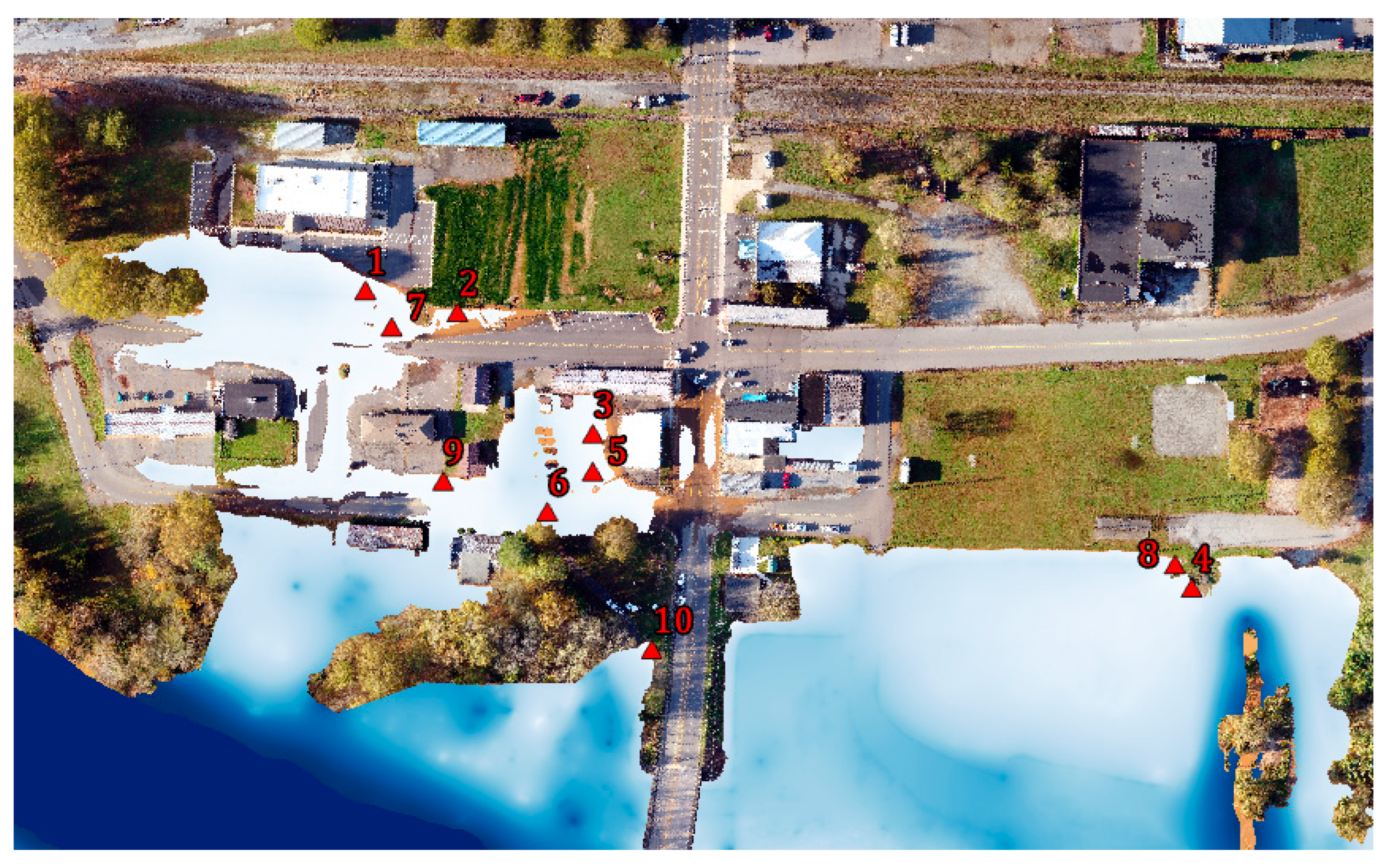
Figure 10.
Floodwater depth measurement locations for depth model validation.

Figure 11.
Floodwater depth maps generated using: (a) FI, (b) PI, (c) FwDET + UAV-DEM, and (d) FwDET + LiDAR.
Figure 11.
Floodwater depth maps generated using: (a) FI, (b) PI, (c) FwDET + UAV-DEM, and (d) FwDET + LiDAR.


Table 1.
Spectral profile of floodwater pixels for overbank and channel flow.
| Band | Name | Extraction Range (DN) | Source |
|---|---|---|---|
| 1 | Blue | 0.38–0.91 | Phantom 4 Pro |
| 2 | Orange | 0.16–0.39 | Mapir Survey 3 |
| 3 | Green | 0.24–0.71 | Phantom 4 Pro |
| 4 | Cyan | 0.10–0.26 | Mapir Survey 3 |
| 5 | Red | 0.18–0.44 | Phantom 4 Pro |
| 6 | NIR | 0.17–0.36 | Mapir Survey 3 |
| 7 | NDVI | 0.00–0.18 | Mapir Survey 3 |
| 8 | DSM | ≤270.72 m | Phantom 4 Pro/RTK GNSS Receiver |
Table 2.
Modeled depth comparison for fully integrated and partially integrated models.
| Model | Resolution (Cm) | Inundation % | Depth Range (m) | Mean Depth (m) |
|---|---|---|---|---|
| FI | 3.3 | 25.6 | 0~9.14 | 2.25 |
| PI | 3.3 | 32.7 | 0~5.76 | 1.25 |
Table 3.
Inundation validation—commission error, omission error, and total error.
| Model | Accuracy | Commission Error | Omission Error | Total Error |
|---|---|---|---|---|
| FI | 88.83% | 4.59% | 11.17% | 15.77% |
| PI | 87.84% | 15.84% | 22.69% | 38.53% |
Table 4.
Water depth comparison between measured and predicted from different models.
| Location | Measured | FI | Diff. (cm) | PI | Diff. (cm) |
|---|---|---|---|---|---|
| 1 | 15.2 | 18.3 | 3.1 | 8.3 | −6.9 |
| 2 | 3.1 | 3.1 | 0.0 | 0.4 | −2.7 |
| 3 | 3.1 | 6.1 | 3.1 | 7.7 | 4.6 |
| 4 | 21.3 | 27.4 | 6.1 | 27.4 | 6.1 |
| 5 | 15.2 | 12.2 | −3.1 | 14.9 | −0.3 |
| 6 | 39.6 | 45.7 | 6.1 | 26.4 | −13.2 |
| 7 | 9.1 | 9.1 | 0.0 | 12.5 | 3.4 |
| 8 | 12.2 | 15.2 | 3.1 | 19.8 | 7.6 |
| 9 | 9.1 | 6.1 | −3.0 | 0 | −9.1 |
| 10 | 12.2 | 15.2 | 3.1 | 70.2 | 58 |
| Average | 14.0 | 15.9 | 1.8 | 18.76 | 4.75 |
Table 5.
Accuracy and error comparison by land-cover type from different models.
| Land Cover | Fully Integrated Model | Partially Integrated Model | |||||
|---|---|---|---|---|---|---|---|
| % Cover | Omission | Commission | Correct | Omission | Commission | Correct | |
| Tree Cover | 12.4 | 34% | 10% | 55% | 35% | 14% | 51% |
| Grassland | 3.6 | 10% | 6% | 84% | 2% | 24% | 74% |
| Built-Up | 44.9 | 17% | 13% | 70% | 5% | 41% | 54% |
| Cropland | 4.3 | 3% | 2% | 95% | 58% | 17% | 25% |
| Bare/Sparse Vegetation | 24.2 | 26% | 14% | 60% | 18% | 36% | 46% |
| Water Bodies | 10.6 | 15% | 7% | 78% | 14% | 6% | 80% |
Table 6.
Water depth comparison in cm between measured and predicted for FwDET-related models.
| Location | Measured | FwDET + UAV-DEM | Diff. | FwDET + LiDAR | Diff. |
|---|---|---|---|---|---|
| 1 | 15.2 | 19.7 | 4.5 | 23.2 | 8.0 |
| 2 | 3.1 | 5.0 | 1.9 | 8.5 | 5.4 |
| 3 | 3.1 | 15.3 | 12.1 | 3.8 | 0.7 |
| 4 | 21.3 | 0.6 | −20.7 | 5.8 | −15.5 |
| 5 | 15.2 | 0.0 | −15.2 | 28.6 | 13.4 |
| 6 | 39.6 | 0.0 | −39.6 | 0.0 | −39.6 |
| 7 | 9.1 | 3.3 | −5.8 | 6.4 | −2.7 |
| 8 | 12.2 | 0.0 | −12.2 | 8.4 | −3.8 |
| 9 | 9.1 | 1.0 | −8.1 | 11.1 | 2.0 |
| 10 | 12.2 | 14.6 | 2.4 | 72.5 | 60.3 |
| Average | 14.0 | 5.9 | −8.1 | 16.8 | 2.8 |
Disclaimer/Publisher’s Note: The statements, opinions and data contained in all publications are solely those of the individual author(s) and contributor(s) and not of MDPI and/or the editor(s). MDPI and/or the editor(s) disclaim responsibility for any injury to people or property resulting from any ideas, methods, instructions or products referred to in the content. |
© 2023 by the authors. Licensee MDPI, Basel, Switzerland. This article is an open access article distributed under the terms and conditions of the Creative Commons Attribution (CC BY) license (https://creativecommons.org/licenses/by/4.0/).
Share and Cite
MDPI and ACS Style
Wienhold, K.J.; Li, D.; Li, W.; Fang, Z.N. Flood Inundation and Depth Mapping Using Unmanned Aerial Vehicles Combined with High-Resolution Multispectral Imagery. Hydrology 2023, 10, 158. https://doi.org/10.3390/hydrology10080158
AMA Style
Wienhold KJ, Li D, Li W, Fang ZN. Flood Inundation and Depth Mapping Using Unmanned Aerial Vehicles Combined with High-Resolution Multispectral Imagery. Hydrology. 2023; 10(8):158. https://doi.org/10.3390/hydrology10080158
Chicago/Turabian StyleWienhold, Kevin J., Dongfeng Li, Wenzhao Li, and Zheng N. Fang. 2023. "Flood Inundation and Depth Mapping Using Unmanned Aerial Vehicles Combined with High-Resolution Multispectral Imagery" Hydrology 10, no. 8: 158. https://doi.org/10.3390/hydrology10080158
Note that from the first issue of 2016, this journal uses article numbers instead of page numbers. See further details here.