Article

Development of Predictive Models for Water Budget Simulations of Closed-Basin Lakes: Case Studies of Lakes Azuei and Enriquillo on the Island of Hispaniola

by
Mahrokh Moknatian
1 and
Michael Piasecki
2,*
1
The Institute for Sustainable Cities, CUNY Hunter College, New York, NY 10065, USA
2
Department of Civil Engineering, CUNY The City College of New York, New York, NY 10031, USA
*
Author to whom correspondence should be addressed.
Hydrology 2021, 8(4), 148; https://doi.org/10.3390/hydrology8040148
Submission received: 12 August 2021 / Revised: 28 September 2021 / Accepted: 30 September 2021 / Published: 2 October 2021
(This article belongs to the Special Issue Hydrology in the Caribbean Basin)

Abstract

:
The historical water level fluctuations of the two neighboring Caribbean lakes of Azuei (LA) and Enriquillo (LE) on Hispaniola have shown random periods of synchronous and asynchronous behaviors, with both lakes exhibiting independent dynamics despite being exposed to the same climatic forces and being directly next to each other. This paper examines their systems’ main drivers and constraints, which are used to develop numerical models for these two lakes. The water balance approach was employed to conceptually model the lakes on an interannual scale and examine the assumptions of surface and subsurface processes. These assumptions were made based on field observations and prior studies. The developed models were optimized and calibrated for 1984 to 2017 and then validated for the period 1972 to 1984 based on the lakes’ observational volume change and volume time series. The models yielded “good” performance, with NSE averaged at 0.7 and RE averaged at 13% for volume change. The performance improved to “very good” for volume simulations, with NSE averaging higher than 0.9 and RE averaging at 1%. The uncertainty analysis showed a p-factor of 0.73 and an r-factor of 1.7 on average, supporting the reliability and precision of the results. Analyzing the time series of the lakes and quantifying the main elements of the water balance, each lake’s shrinkage and expansion phases were explored, and the drivers of such behavior were identified for each lake. The main drivers of LE’s system are North Atlantic cyclone activities and uncontrolled inter-basin water transfer, and direct rainfall and evaporation to/from its surface. For LA, its system is controlled mainly by groundwater fluxes in and out of it, despite possessing small values in its water budget.

1. Introduction

Closed-basin (endorheic) lakes, identified as “low-pass” frequency filters, exhibit a strong presence of persistent behavior as a response to high-frequency forces exerted by climate [1]. Long-term periods (interannual and decadal scales) of an increase/decrease up to tens of meters on top of the lake’s annual and seasonal oscillations are often standard for such lakes. An example is the 6-m steady rise of Lake Bosumtwi (Ghana) from 1940 to 1980, followed by its steady shrinkage until the mid-2000s [2]. Lake Turkana, located between Kenya and Ethiopia, has gone through similar episodes of expansion and shrinkage, having stable levels during the period 1993–1995, then rising by 4.5 m until 1999, and finally decreasing until 2006 [3,4]. In North America, the Great Salt Lake is characterized by its long-term cycles. The lake’s water level time series shows a decrease of 3 m during the 1950s and 1960s, followed by a 6 m increase in the mid-1980s, and then another episode of shrinkage resulting in a 5 m drop in 2010 [5]. Devil’s Lake in North Dakota had a declining pattern, losing 12 m of water between 1860 and 1940 before experiencing a significant rise in water level (+15 m) in the 1940s [6]. In Central Argentina, a 7-m rise was observed for Lake Mar Chiquita from 1970 to the mid-1980s [7]. On the island of Hispaniola, Lake Azuei (LA) and Lake Enriquillo (LE) (our case study sites) both started to grow unexpectedly from 2004 to 2014, rising about 3.7 m and 10.4 m, respectively [8].
A fundamental and widely used tool for better understanding the fluctuations of lakes is water balance modeling, through which the physical relationship between climatic and hydrological variables is quantified. The main water balance components of closed-basin lakes are precipitation, evaporation, surface fluxes (e.g., runoff and streamflow), and subsurface fluxes (e.g., groundwater and lateral flow). While climatic variables are often quantified using direct measurements, surface and subsurface fluxes (known to be dominant factors in some closed-basin lakes’ water level variations) have to be crafted and formulated in the manner most suitable for the specification of the watershed under study. For example, surface fluxes were the dominant factor in lakes Keilambete and Bullen Merri, Australia [9]. The decadal rise of Lake Mar Chiquita was attributed to the increased runoff in the upper northern sub-basin [7]. The growth of lakes Selin and Qinghai (Tibet) from 2002 to 2010 was related to increased glacial runoff [10]. Other examples are the glacial lakes of Redernswalder and Krummer See (both in Germany), for which groundwater, along with precipitation, was identified as one of the main drivers of their dynamics [11]. Surface fluxes are generally included in the water-balance modeling of closed-basin lakes because of their proven significance and quantification feasibility. Depending on the availability of data, many different methods have been developed to estimate runoff directly from measurements or indirectly from its relationship with other already available water balance variables (e.g., precipitation [12,13,14,15] and evapotranspiration [2,16,17]).
Conversely, subsurface flows are often assumed to be negligible in most studies despite their essential role in stabilizing closed-basin lakes, especially in semi-arid regions [18,19,20]. The main reason for this assumption is the lack of understanding regarding subsurface processes and the difficulty in measuring and quantifying them (e.g., [2,3,6,12,14,15,21,22,23]). In studies where substantial groundwater inflows were present in the mass balance calculations, chemical mass balance (chloride) was employed for groundwater estimations (e.g., [7,24,25]). Other studies have attempted to gather observations in the field, such as piezometric measurements from wells and boreholes (e.g., [9,11]). However, research on subsurface fluxes for groundwater-dominated flows into endorheic lakes is poorly developed, primarily because of insufficient data.
For this case study (Lakes Azuei and Enriquillo), the role of subsurface fluxes in controlling the lakes’ water level fluctuations is essential, yet no hydrogeological field measurements are available to estimate groundwater contributions to the lakes’ water budget. When comparing the interannual growth rate of the lakes’ water levels around the globe, LA’s growth rate of 0.3 m per year (m/yr) falls within the average ranges; however, LE’s rise of 1 m/yr for ten consecutive years exhibits one of the highest rates globally (after Lake Turkana, which rose by 4.5 m from 1996 to 1999 [3]). The unexpected expansion of these two lakes has imposed significant environmental and socio-economic complications on the region, creating an urgency for the government to address the adverse effects of this phenomenon, resulting in the deprioritization of comprehensive data collection campaigns. This, coupled with financial restrictions on such campaigns, has severely impacted the scope of modeling efforts.
It should be noted that none of the previously mentioned studies considered including subsurface fluxes in cases of insufficient hydrogeological data, leaving no guidelines and pointers on how to conduct lake water budget modeling in cases of scarce data. In addition, the different dynamics of LA and LE before their constant rise during the period 2004–2014 show the necessity of focusing on surface and subsurface fluxes because the climatic drivers on their systems are the same. Adding to the scientific discussion and knowledge pool, the paper attempts to introduce formulae and numerical models to include surface- and subsurface fluxes developed solely from available long-term precipitation data and the essential characteristics of the lake basins. In this approach, multiple runoff coefficients were introduced to account for precipitation intensity and soil moisture conditions at the time of precipitation to improve surface flux estimations. In the presence of subsurface fluxes, the paper develops a linear relationship between these fluxes and the water depth present on top of the soil at the time of precipitation. The manuscript outlines the necessary data analysis and reverse engineering to formulate the water depth based on precipitation to emulate each lake’s dynamics best. The outlined steps and strategies are novel developments and are unique to the discussion on endorheic lakes.
The key objectives were to understand better the main drivers and constraints of the lakes’ systems and provide answers to critical questions raised by the scientific and local communities, including, but not limited to: (i) What was the cause of the lakes “great” expansion? (ii) What is the reason behind their different dynamics? (iii) How can their historical expansion and shrinkage patterns be explained? (iv) How much was the contribution of each water balance component?

2. Materials and Methods
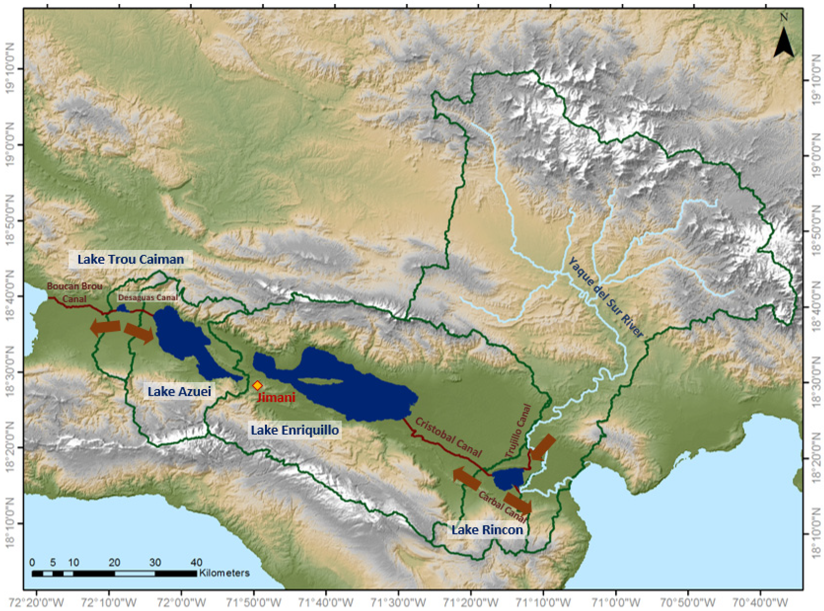
2.1. Study Area

Hispaniola, where LA (also called Etang Saumatre) and LE are located, is characterized by valleys and mountain ranges stretching east to west. The valley on the south of the island is called the Cul de Sac depression on the Haitian side and the Enriquillo plain on the Dominican Republic side [26]. LE is located in the lowest part of the valley, about 33.2 m below mean sea level (MSL), covering an area of 325.3 km2 (November 2017), and having two deep sections in the north and south with shallow edges on the west and east [27]. About five kilometers to the west of LE lies LA at about 23.0 m above MSL, with a surface area of 134.75 km2 (November 2017) and steep banks around its shoreline [27]. Both lakes are saline in nature, with LE’s salinity level being higher (34 ppm) than LA’s (7–9 ppm, reducing to <5 ppm in the vicinity of subsurface springs). The lakes are endorheic (“topographically closed-basin”), i.e., they have no surface outlet to the sea and are fed by their surrounding watersheds. Figure 1 shows the two lakes and their associated watersheds. During the lake expansions from 2003 to 2014, LE had unprecedentedly expanded to twice its size, and LA had grown by 20%. While climatic drivers on LA and LE systems are the same, their interannual dynamics and seasonal fluctuations are different, despite their proximity to each other. Looking beyond their aligned behavior during 2003–2014, LA grew by 5% in size, while LE was shrinking during 1993–1996. From 1979 to 1982, LE experienced a 3 m rise, followed by prolonged shrinkage; however, LA’s level exhibited a steady-state equilibrium [28]. Time series analysis of LE’s fluctuations has also shown its seasonal sensitivity to rainfall intensity, while LA solely responds to rainfall magnitude (not seasons) [29].
The streams around both lakes are ephemeral, and each lake is located in approximately the center of its respective basin. The area encompassing both lakes’ watersheds covers 3867 km2, of which 805 km2 belong to the Azuei basin and 3062 km2 to the Enriquillo basin. Both watersheds are surrounded by mountains ranging from 2100 m MSL in the northern Sierra (Neiba) to 2660 m MSL in the southern Sierra (Bahoruco). The terrain is covered by bands of forests, including the Montane forest region while being treeless in higher elevations. Climatic variations range from semi-arid, covering the plain area around LE and LA, to very humid in the mountainous Sierras [30], ranging from 20 °C to 36 °C [31]. The climate of the study area is characterized by two rainy seasons (long and short), alternating with two dry seasons. The rainy seasons occur in the spring (April–June) and autumn (September–November), and dry seasons occur in summer and winter [30,32]. The average annual rainfall on LA varies between 663 and 814 mm at lower altitudes, while the higher areas are subject to much greater rainfall rates, with average annual precipitation between 1230 mm to 2590 mm [32]. Annual rainfall near LE ranges from 508 mm to 729 mm [33], increasing gradually with elevation until about 1100 m and diminishing again for higher elevations [34].
The Bahoruco and Neiba mountains around the lakes are characterized as having high permeability rock formations. These mountain ranges are composed of calcareous (limestone) soil and have a well-developed karstic structure favoring high infiltration rates [35]. The Bahoruco Mountains feed the springs on the south side towards the Caribbean, while the Neiba Mountains direct the water to the springs inside the Enriquillo watershed, which is located on the north side of the town of Neiba [36]. However, the alluvium aquifer of the Enriquillo Depression, situated between Bahoruco and Neiba, receives only a minor amount of recharge [36].
In the 1950s, LE experienced a significant recession of its water levels, which prompted the construction of several canals to divert water from the Yaque del Sur River, one of the Dominican Republic’s main rivers [37]. The Trujillo Canal diverts water from the River to Lake Rincon (also called Cabral Lagoon), from where the Cristobal Canal guides the flow towards LE (Figure 1) [30,38,39,40,41,42,43,44,45]. This canal system connects the two watersheds of Yaque del Sur River and Lake Rincon to LE, causing inter-basin water transfer and, consequently, partial drainage into LE. In the late 1960s, for irrigation reasons, Trujillo Dike was constructed to block the water transfer from Yaque del Sur to LE, disconnecting the river’s watershed from that of Lake Rincon and LE [46]. The Haitian side has also experienced inter-basin water transfer towards LA through the canal system built in the early 20th century [47]. The Desaguas Canal, situated on the east side of Lake Trou Caiman, drains the water into LA, while the Boucan Brou Canal extends on the west side of Trou Caiman, discharging into the sea (Figure 1). This canal system was constructed to drain the water away from Lake Trou Caiman to protect the town of Thomazeau from flooding during extreme rainfall events.

2.2. Data Availibility

A key challenge for this study was the scarcity of long-term hydroclimatic data, e.g., evaporation; relative humidity; wind; solar radiation; and spatially distributed information on soil, land cover, groundwater, and, to a lesser extent, precipitation and temperature. The primary source of datasets was the Oficina Nacional de Meteorología (ONAMET) in the Dominican Republic, the National Observatory of Environment and Vulnerability (in french: ONEV) in Haiti, and the Coastal Urban Environmental Research Group (CUERG) at the City College of New York. There were/are 38 meteorological stations in the study area, 23 of which were installed by CUERG in the northern and southern mountain ranges surrounding Lake Enriquillo, which have been providing data records since 2012 with inter-daily intervals. The ONEV stations in Haiti also provided records on an inter-daily basis from 2011 to 2014. However, the records provided by the stations above were mostly unprocessed data containing many gaps, i.e., uneven and inhomogenous data availability at temporal and spatial scales, rendering them insufficient for this study. The data provided by ONAMET, on the other hand, were mostly comprised of monthly processed data from several stations inside the Enriquillo watershed, among which there was only one station (Jimani, shown in Figure 1) with long-term data coverage. The vicinity of Jimani station to both LA and LE made it a geographically suitable representative of the climatic conditions inside the lakes’ watersheds. Among all the data attributes collected, monthly precipitation data was the only attribute having long-term and consistent information with the fewest data gaps for 1963–2017, satisfying the 40-year modeling requirement for this study.
Other datasets that supported the work were the lakes’ monthly volume and surface area time series from 1972 to 2017 [8,27,28]. These datasets were derived from Landsat Imagery analysis and two field campaigns conducted in 2013 by CUERG for bathymetry surveys of the lakes [48]. The parameter values needed for configuring the models were estimated using information collected from various sources and are explained in detail in the next section.

2.3. Model Development

Due to the scarcity of hydrogeological data in this study’s geospatial and temporal domains, the decision was made to develop a water budget model rather than establish a geospatially distributed model such as GSSHA, SWAT, or MIKE-SHE (among others). Because previous research has shown that yearly averages are a suitable indicator for long-term ecological changes [49,50,51], the model development focused on the production of yearly time series. The model is comprised of a water budget balance ( V , change in volume) that, in its rudimentary form, can be written as:
Δ V Δ t = L + W + H + G + I
where L, W, H, G, and I are lake, watershed, hydrological interactions of Azuei and Enriquillo, groundwater, and inter-basin water transfer components, respectively.
Volume Change ( V t ): The volume time series of both lakes have been previously developed using satellite imagery from 1972 to 2017 [8,28]. Hence, the interannual time series of each lake was extracted (Figure 2), from which yearly volume change values (mm/yr) were computed. Lake volume change quantities and other known parameters of the water balance equation were estimated and used to develop the models to simulate the lakes’ hydrological behavior.
Lake Component (L): This component involves direct rainfall and evaporation over and from the lake’s surface and is defined as:
L = ( P L E L ) A L
PL and EL are direct precipitation, and evaporation rates (mm/yr) over and from the lake, and AL is the lake’s surface area. Direct rainfall over the lakes was assumed to be equal to the Jimani (a town located between the lakes, shown in Figure 1) station rainfall due to its location between both lakes. For evaporation, constant average values of 1250 mm/yr and 1400 mm/yr were considered for LE and LA, respectively, throughout the simulations. While values were derived from several sources, emphasis was given to the data published by PRAGWATER [52], from which method based (Priestly-Taylor, Penman-Monteith, and Hargreaves-Samani) yearly average values were computed. Given the insignificant variation in regional temperature, preliminary analysis showed that the monotonic increase/decrease in evaporation (which might be a sign of climate change) could not explain the fluctuations of the lakes. Therefore, constant evaporation rates were assumed to prevail throughout the simulations for lack of time-variant information.
Watershed Component (W): the watershed component refers to the watershed surface runoff contributing to the lake’s water budget. The runoff formula [1,53] employed in this study is as follows:
W = r c P w A w
where rc is runoff coefficient, Pw is precipitation rate (mm/yr) over the watershed, and Aw is the watershed surface area excluding the lake (area over which runoff is collected). Despite the simplicity of this equation, it has been employed in many studies, showing its applicability, especially for watersheds with ephemeral streams and when comprehensive information regarding surface hydrology is not available (e.g., [15,54]), the parameter of rc accounts for processes such as evapotranspiration and groundwater percolation that affect runoff production. In most studies, rc is kept constant, even though its value varies depending on precipitation rate and soil moisture at the time of a rainfall event [14,53,55].
For years with average precipitation, it has been suggested that runoff is low for stations that are located at lower altitudes in the Enriquillo watershed [35,56]. Conversely, field observations show that substantial runoff occurs during storms, causing flooding of the region [35]. Based on these observations, two different runoff coefficients were considered for Enriquillo’s water balance calculations: rc1 for years without storm and rc2 for years with storm occurrences, to account for the influence of rainfall intensity and soil moisture at the time of an extreme event. Impactful storms on LE’s water balance are identified in an 80 km radius of its watershed when they introduce more than 87 mm of precipitation [29]. The reader is referred to [29] for the list of North Atlantic storms sufficiently heavy to affect LE’s water balance. No extreme runoff events have been reported for Lake Azuei, and preliminary analysis suggested the use of a constant runoff production value after each rainstorm event. Therefore, only one runoff coefficient was considered in the runoff calculation. Initial values were assigned to be between 0 to 0.60 for both watersheds [57,58], which were then improved to yield optimized values during the lake models calibration process.
It was also assumed that (a) runoff coefficients stayed constant throughout the study period and (b) that the continued worsening of deforestation played no significant role. The latter assumption was not unreasonable because both watersheds are already greatly denuded [59,60], and the introduction of a hypothetical monotonic change of deforestation did not yield any significant changes in the lake volume changes.
Using data obtained from meteorological stations in Haiti and the Dominican Republic and subsequently producing a hyetograph map of the study area, rainfall ratios over the surface of each watershed were estimated to account for the variance of precipitation rate for each elevation band. Results showed that the Azuei watershed received 37%, and the Enriquillo watershed 7% more precipitation than the corresponding lake surface. This phenomenon was due to the orographic precipitation effect, enhanced by the topography of the study area.
Hydrological interactions of lakes Azuei and Enriquillo (H): A connection between the two lakes has been shown to exist (field observations in 2013 and 2014; identification of springs), which discharges water from LA towards LE. It has been speculated that this gradient could significantly contribute to LE’s 2003–2014 growth, even though no attempts to quantify the springs’ flow rate have ever been undertaken. The hydrogeological dynamics were conceptualized by considering a schematic cross-section that cuts from LA, through the peninsula, to the western shore of LE, with a typical water table drawn between the two lakes, as shown in Figure 3a. The spring locations are approximately at the −37 m (MSL) mark. Records show that LE’s historical water level fluctuations range between −42 m to −31 m MSL, and LA’s historical surface elevation ranges between 19 m to 23 m MSL [28]. The fluctuations of the lakes suggested that the springs were submerged when LE’s level was above −37 m, thus altering the hydraulic gradient between the lakes, as shown Figure 3b. For modeling the lakes, the term H represents the discharge volume exchanged between the lakes. Because the flow direction is from LA to LE, this term was set to zero in the LA water balance equation. However, for LE, it had to be estimated, which is addressed next.
The lake dynamics introduced an additional feature on the LA’s system in which the up-and-down of LE created a feedback mechanism for LA, influencing the hydraulic gradient and thus the flow rates. However, the feedback mechanism is not only based on the hydraulic gradient between the lakes but also on the groundwater interactions between the lake proper and its surrounding watershed areas.
Groundwater Component (G): It is safe to assume that the amount of flow into and out of the lake is balanced; therefore, groundwater contribution equals zero when the lake is in an equilibrium state [1]. For periods when the lakes are not in an equilibrium state, groundwater interactions need to be calculated. These groundwater interactions were estimated using a linear empirical approach that expresses as a fraction of the water depth present at the top of the soil over a yearly period (PD), which then percolates into the deep aquifer and eventually ends up in the lake.
G = i n f c P D A w
where infc is a dimensionless average infiltration coefficient [-]. infc was determined (weighted average) to be 0.19 for the Enriquillo and 0.21 for the Azuei watershed, which was based on the composition of mountainous and plain areas for each watershed [61]. To emulate the characteristics of the lakes, employing extra constraints proved to be necessary during the preliminary modeling attempts.
For LE, historical observations show that the lake continued to grow for several years after storm activities, despite the low rainfall rates that were observed for those years [37]. Because there were no observed significant surface runoffs during these years, it was clear that there must be significant sub-surface flows originating from “stored” mountain-side water volumes that continued to reach the lake with a considerable time lag. Conversely, shrinkage of the lake during consecutive years without impactful storms indicated negligible contributions from groundwater recharge (G ≈ 0). Therefore, groundwater contribution was only considered for the years following an impactful storm incident with a one-year lag time and PD equal to Pw. It should be noted that groundwater return flow was added to the water balance for eight consecutive years (LE’s response time [29]) following the storm, starting from an initial value of i n f c P D A w and decreasing exponentially. Moreover, Pw had to be set to monthly rainfall caused by the storm over the watershed and not the cumulative annual rainfall.
Historical observations for LA showed a much more muted response signature to storm incidents [29]. The lake’s fluctuations, in general, aligned more with yearly precipitation patterns. Analysis of the volume change time series from 1972 to 1992 showed that the lake’s volume remained constant for rainfall rate between 800 to 1200 mm/yr over the watershed surface (~600 to 800 mm/yr recorded at the Jimani station). For precipitation beyond this range, the lake showed (minor) departures from its equilibrium state. This relatively stable behavior of LA was attributed to the role of groundwater as a central regulator of the watershed’s water balance. As a result, the PD value was determined to be the difference between an equilibrium modifier ( P ¯ w ) and yearly precipitation over the watershed surface (Pw):
P D = ( P ¯ w P w )
The preliminary analysis for LA revealed that, when no external forcing was involved, P ¯ w could be considered equal to the long-term average precipitation. LA had experienced this steady-state equilibrium during two prior periods: between 1972 and 1982 and between 1984 and 1994 (Figure 2), for which P ¯ w was set to be equal to the long-term average precipitation of 1000 mm/yr (~733 mm/yr recorded at the Jimani station).
However, these modifications did not explain the lake’s behavior in 1983 and for the years following 2007. Additional analysis showed that the hydrological connection between the two lakes needed to be accounted for in the estimation of P ¯ w . More specifically, a new LA equilibrium established itself whenever LE experienced surface levels higher than the springs’ location (at –37 m MSL). Consequently, adjustments to P ¯ w were needed. To this end, a linear regression expression to estimate P ¯ w was introduced, which showed a significant correlation between P ¯ w and LE’s rate of elevation change (95% confidence level). Historical lake data showed that the new equilibrium would occur with a one- or two-year delay after LE’s level decreased to levels below –37 m MSL, i.e., a slow response time, as witnessed in the period 1981–1982; while it occurred rapidly, for example, in 2007 when LE rose above –37 m MSL.
Note that the G in LA’s water balance component could possess both negative and positive values depending on the annual rainfall rate, indicating the presence of incoming or outgoing groundwater seepage. To account for the water transfer from LA to LE, whenever the G value in LA’s water balance was negative, all the outgoing seepage was added to LE’s water balance (HLEGLA), although it is clear that not all Azuei seepage would end up in LE. Using the hydraulic gradient formula constitutes a rough assumption because of the difficulty in computing the correct discharge due to inadequate hydrogeological information.
Inter-basin water transfer component (I): The canal systems built around both lakes have caused uncontrolled water transfer toward the lakes, connecting the three neighboring watersheds (Lake Trou Caiman on the Haitian side, Lake Rincon, and Yaque del Sur River on the DR side) to the watersheds of LA and LE (see Figure 1). The inter-basin water transfer component toward the lakes ( I = f Q ) was defined as a fraction (f) of canal discharge volume (Q). For LE, the f factor was either 0 or 1, depending on the absence/presence of Cristobal Canal discharge in each year. Significant Cristobal Canal flow (up to 25 m3/s) was reported for the years following 2007 (when Trujillo Dike on Yaque del Sur River failed due to the previous storm events) up to 2011 (when the dike reconstruction was finished) and then for a few years after that (until 2013). Preliminary analysis of Cristobal discharge also revealed its contribution to LE’s water budget before the Trujillo Dike incident. For example, in 1979, two consecutive storms occurred close to the study area, resulting in a two-year-long flow towards LE, causing a 4-m rise in lake level. Precipitation alone could not explain this rise, which meant an extra discharge was added to LE. Incidentally, satellite imagery for this period confirmed an expansion of Lake Rincon, resulting in additional water transfer to LE. Although the discharge rates varied each year (between 0 and 25 m3/s), the assumption was made that they remain constant throughout all years for simplicity (and lack of reliable Christobal discharge time series). This range was used to calibrate the model, i.e., as an optimization constraint for the Cristobal discharge (0 < QChristobal < 25 m3/s).
On the Haitian side, the determination of the Desaguas Canal discharge towards LA was challenging due to the lack of observations or published data. However, an alternative examination of Lake Trou Caiman’s extent using satellite imagery yielded possible months during which flow towards LA occurred. Analyses yielded an LA flow factor that ranged from year to year from zero to one. The amount of discharge from the Desaguas Canal was determined by adjusting its value through model optimization.
Between 1992 and 1996, during which LA expanded and grew by approximately 5% in volume, preliminary analysis showed that neither the Desaguas discharge nor the LE water level seemed to be fully responsible for such a change. For the sole purpose of modeling, an additional source of discharge, equal to 0.06 km3, was added between 1993 and 1996. However, this rudimentary and ad hoc fix needs to be investigated further.

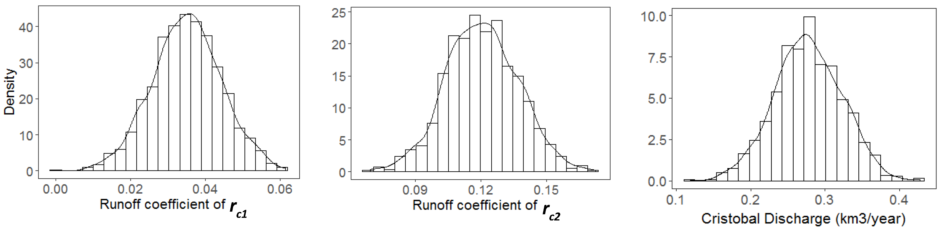
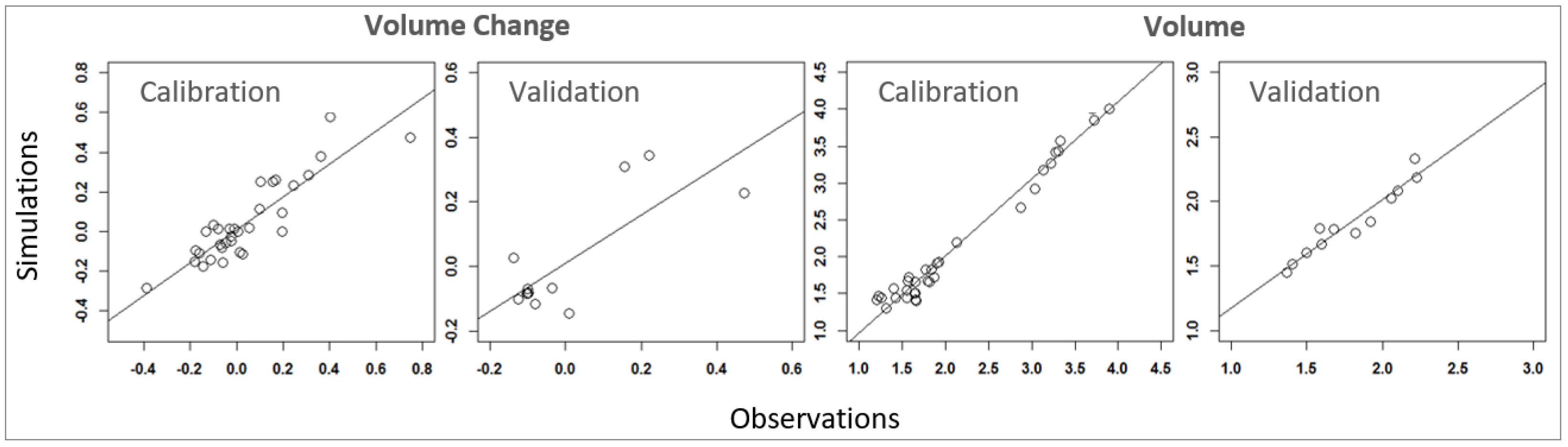
2.4. Model Calibration, Validation, and Uncertainty Analysis

Of the parameters present in the water balance equation, only precipitation, lake volume, lake surface area [28], and watershed surface area data were continuous (1972–2017), with all other variable’s time series only having intermittent data. Filling these data gaps was achieved using long-term averages (i.e., evaporation, infiltration coefficient, and equilibrium modifier) or an optimization routine during the calibration period (i.e., runoff coefficients and inter-basin water transfer). Because LE showed a solid response to forcings by North Atlantic storms and exhibited a much lesser impact on groundwater interactions, while LA showed a solid response to groundwater, two different models (one for LA and one for LE) needed to be developed. The final forms of the water-budget equation for both lakes are as follows:
Lake   Enriquillo : V t = ( ( P L E L ) A L ) + ( r c P w A w ) + ( i n f c P w A w ) + ( f Q ) + G L A where ,   r c :   { r c 1 ,         years   without   storms r c 2 ,               years   with   storms
Lake   Azuei : V t = ( ( P L E L ) A L ) + ( r c P w A w ) + ( i n f c ( P ¯ w P w ) A w ) + ( f Q ) where ,   P ¯ w :   { P ¯ w 1 ,                   no   LE   effect   ( LE   elev   <   37 m ) P ¯ w 2 ,         LE   effect   present   ( LE   elev   37 m )
It should be noted that the values of the variables in Equations (6) and (7) differ despite the same notation used. The time frame between 1972 and 2017 was split into the calibration (1984–2017) and validation (1972–1984) periods. The parameter optimization for the calibration period was carried out utilizing a non-linear optimization algorithm, in which the objective function was set to minimize the root mean square error (RMSE) between observed and estimated volume change. During the optimization process, three parameters (rc1, rc2, and Q) for LE and two parameters (rc and Q) for LA, were adjusted to yield the best match between model and observed lake storage changes. Interannual volume time series of the lakes were simulated for the calibration and validation periods using a parameterized model. The model performance quantification and uncertainty analysis were carried out for estimated volume and volume change values. For model performance, the estimated values were compared to the observations. The uncertainty analysis was performed by computing a 95% prediction uncertainty (95PPU) method proposed by [62] for volume and volume change time variables.

2.4.1. Lake Enriquillo-Model

The optimization process yielded values of 0.035 ± 0.009 for rc1 (runoff coefficient during years with no impactful storm event), 0.121 ± 0.016 for rc2 (runoff coefficient during storm years), and 0.2769 ± 0.045 km3/yr for the volume of water added via the Cristobal discharge (Q), with a root mean square error (RMSE) of 0.58. Uncertainty analysis using the Monte Carlo method showed that the 95% percentile intervals of rc1 and rc2 were (0.0344, 0.0355) and (0.1195, 0.1215), respectively. For Q, the 95% percentile fell within 0.2741 and 0.2797 km3/yr (equivalent to 8.69 and 8.87 m3/s), with mean value of 0.2769 km3/yr (~8.78 m3/s). The distributions of these parameters are shown in Figure 4.
A parameterized volume time series of the lake was constructed using optimized values of rc1, rc2, and Q that were obtained from a year-by-year alteration of the values. This procedure accounted for the propagation of uncertainty throughout simulation years. The volume simulations were conducted separately for calibration (starting from 1994 and moving to 2017) and validation (starting from 1994 backward to 1972). The model’s performance was evaluated using the residual sum of squares (RSS), root-mean-square error (RMSE), mean absolute error (MAE), relative error (RE), and the Nash–Sutcliffe Efficiency (NSE) coefficient. The p-factor and the r-factor [62] were included in the performance analysis to examine how well the 95% prediction uncertainty performed in enveloping the observations. Table 1 summarizes the calibration and validation performance analysis.
Generally, an RE between ±10% and an NSE between 0.75 and 0.8 indicates an excellent model performance [63]. While the model performance in simulating volume changes fell within “good” bounds, the model performed exceptionally well (“very good”) when computing volume values with an NSE of more than 0.9 and an RE less than 5% for both validation and calibration periods. Figure 5 shows both estimated volume and volume change values graphed against observations.

2.4.2. Lake Azuei-Model

Using a Monte Carlo type approach, optimization of the LA water balance model produced runoff coefficient and Desaguas discharge of 0.1097 ± 0.01 and 338.2 ± 319 lit/s, respectively; for parameter distributions, see Figure 6.
The runoff coefficient showed a normal distribution, while the Desaguas discharge density distribution showed a predominantly zero value; the frequency for values other than zero was much smaller, with only slight variations. As a result, the discharge value was not applied through the entire time series; instead, its value was optimized separately for each temporal sub-period. The 1984–1992 sub-period yielded an optimized discharge value of zero, while the 1996–2017 sub-period yielded a constant value of 338 lit/s. Model simulations were compared with observational data to quantify the model performance, following the same process described for LE. The results are summarized in Table 2 and are also shown in Figure 7.
Overall, model performance was excellent considering the small error value of RE averaging at 7% and NSE averaging at 0.8 for volume change and volume. However, for the validation period, the values for the r-factor showed a higher level of uncertainty than expected (5.54 for volume change and 2.51 for volume). This is because LA’s volume change possessed minimal values (less than ±0.01), with a median of zero for 1972 to 1984. During those years, the changes of the lake were undetectable from the observational time series. Therefore, 50% of the observed volume change values were obtained to be zero because the values were extracted from satellite imagery with a 30 m resolution. Note that the lake must have fluctuated, albeit by a minimal amount (which is captured in the model simulations). The water budget parameter values for LA and LE are summarized in Table 3.

3. Results

3.1. Water Budget Assessment

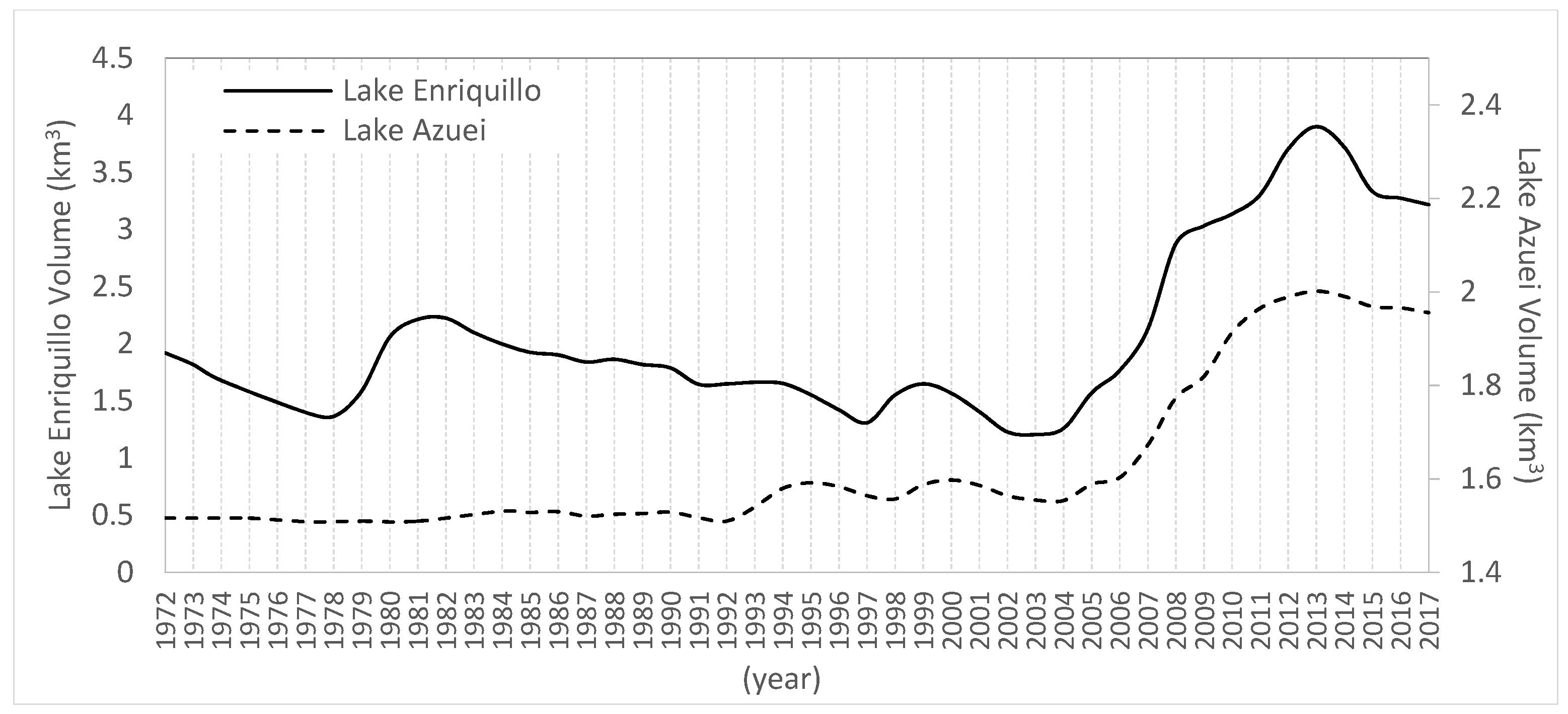
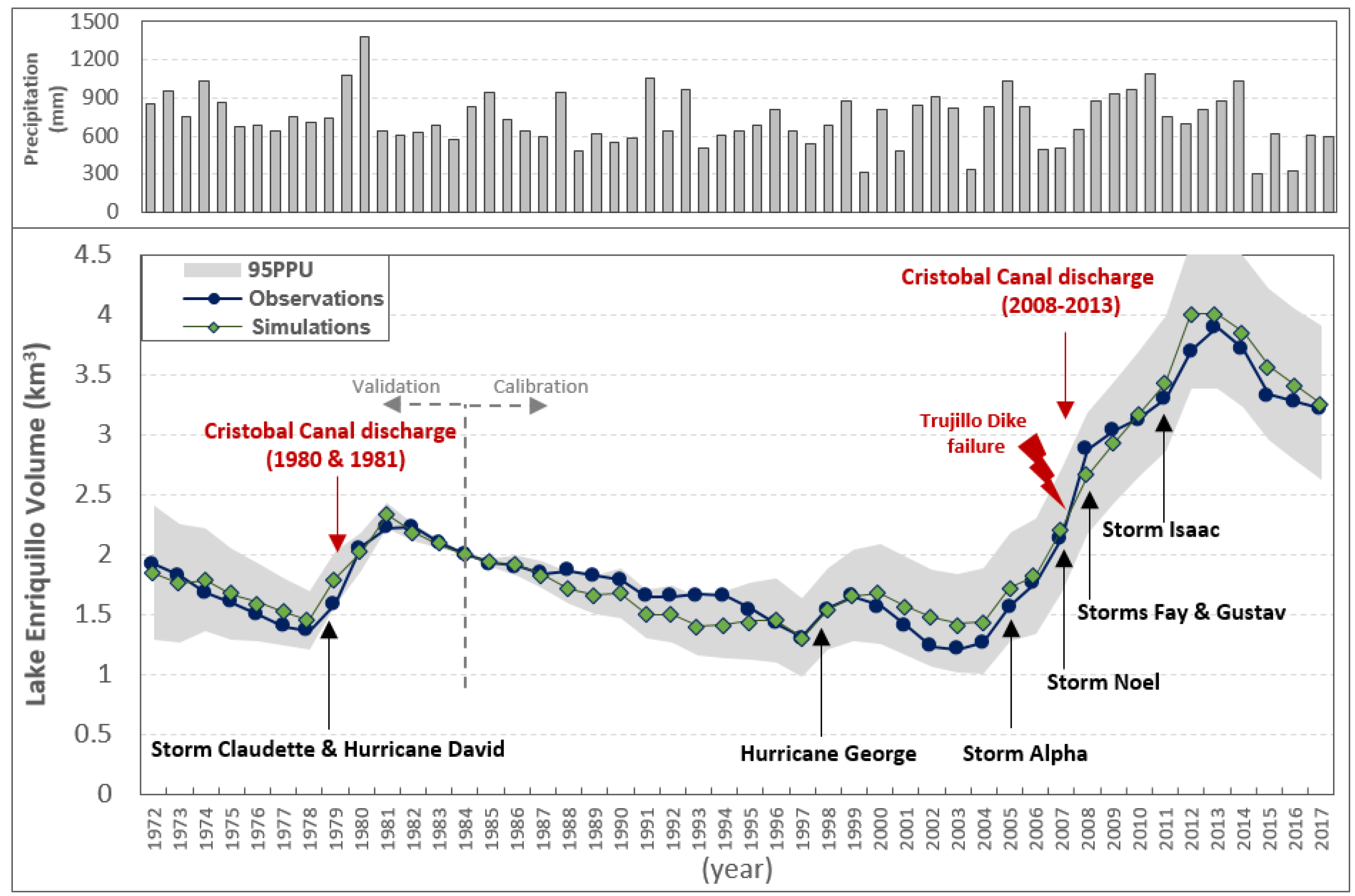
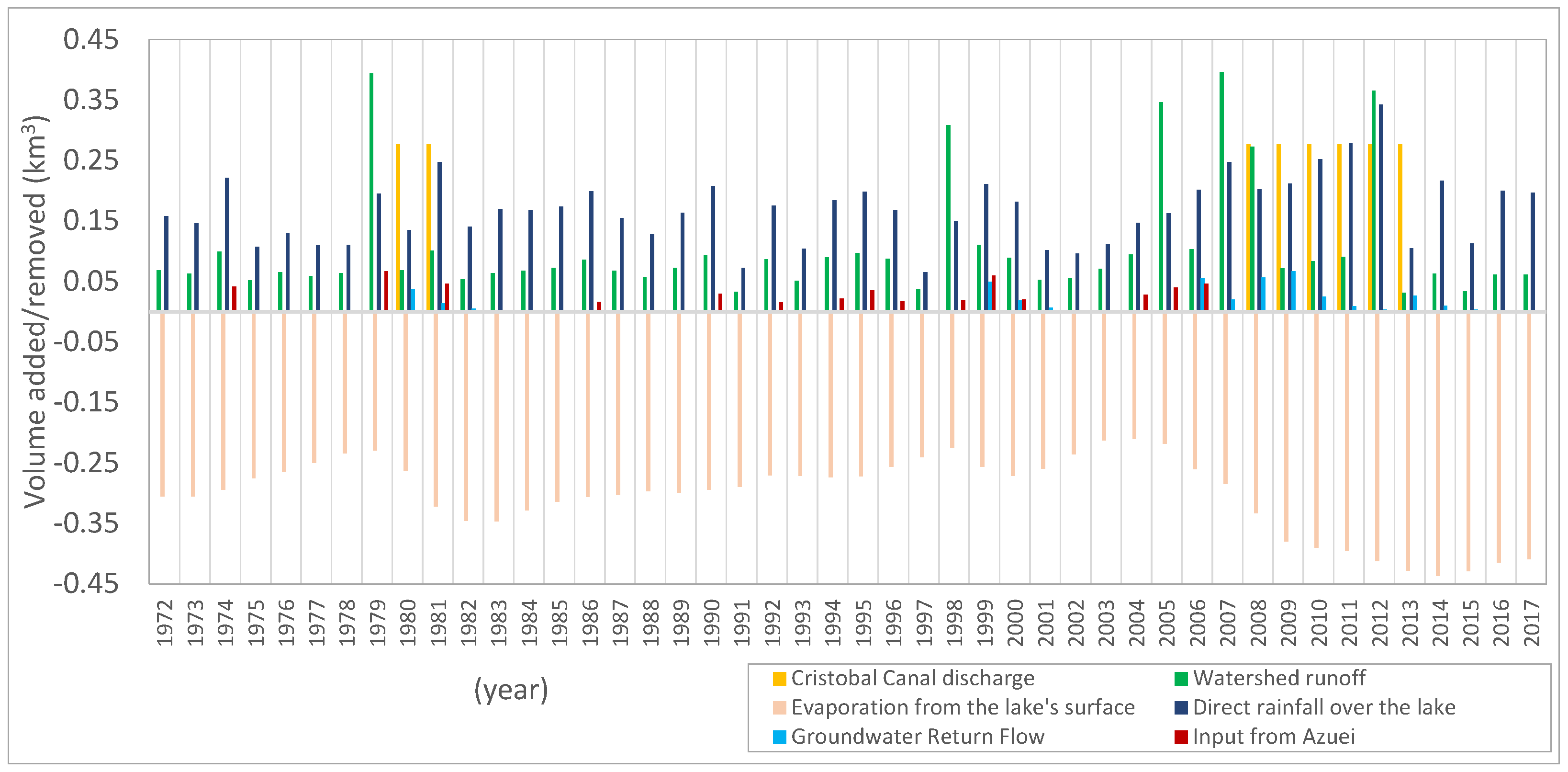
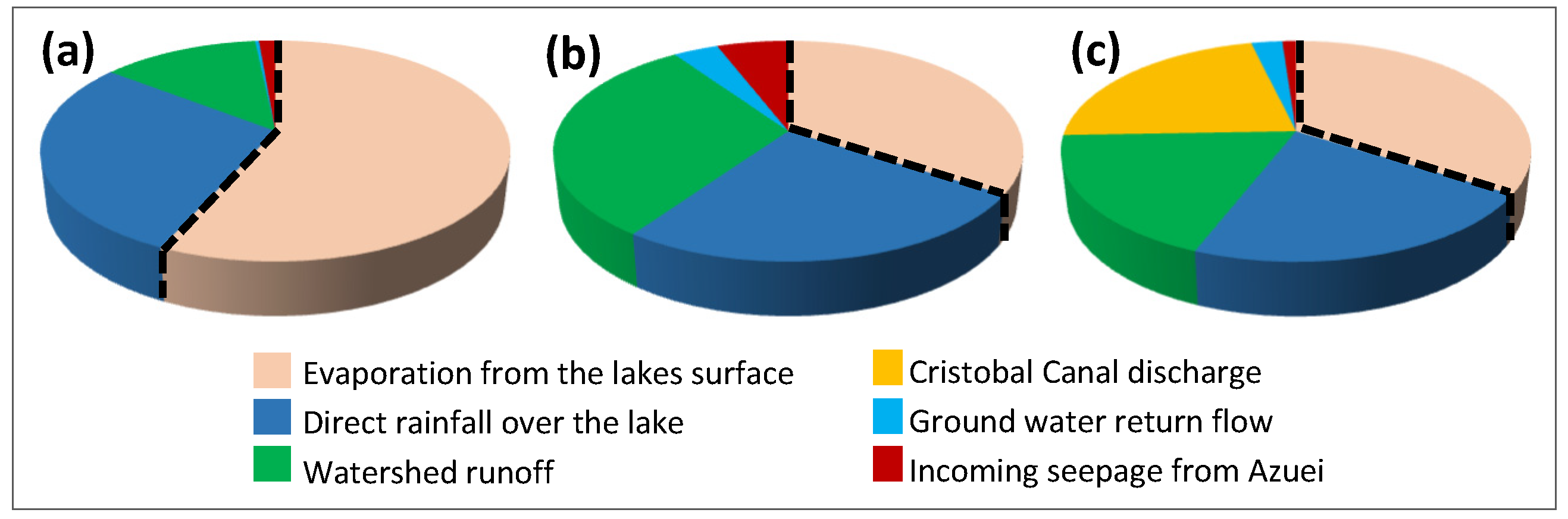
3.1.1. Lake Enriquillo

Plotting the model and observed time series side-by-side (Figure 8) shows how well the model reproduces the observed time series. In this figure, the external forces of North Atlantic Storms and Cristobal Canal discharge are also depicted for the dates they occurred. Another component impacting LE’s water budget, which could also be categorized as an external force, was incoming seepage from LA. This component is not shown in Figure 8 because of: (a) its minor impact on LE’s volume change; and (b) its distributed nature throughout time. The LE water budget components were computed, re-categorized, and graphed for every year (Figure 9). The new water balance components are volume added to the lake from direct rainfall, watershed runoff, groundwater return flow, Cristobal Canal discharge, inflow from LA, and volume removed from the lake through evaporation. Although evaporation was kept constant throughout the simulations, its volume varied depending on the lake’s surface area (peach-colored bars with negative values in Figure 9).
To better explain Enriquillo’s water budget and behavior, the time series is divided into eight sub-periods:
1972–1978:
This period was characterized by a shrinkage pattern. No storm activities occurred close to the region, and the evaporation rate surpassed inflow to the lake from rainfall and surface runoff (with direct rainfall volume being higher than runoff). Therefore, the lake’s water budget was negative, and the lake was shrinking. For this period, the average direct rainfall volume rate was 0.14 km3/yr, the runoff was 0.07 km3/yr, and evaporation was 0.28 km3/yr.
1979–1981:
In 1979, Storm Claudette and Hurricane David hit the area close to the lakes within a few months, causing the lake to grow due to high surface runoff volume. Later, flow brought by the Cristobal Canal from the neighboring watershed (Lake Rincon) added to the expansion, causing the lake level to rise by 4 m in total (which, otherwise, would have been 2.5 m). The amount of runoff caused by storms in 1979 was estimated to be 0.39 km3, while the cumulative volume of water from the Cristobal Canal was 0.55 km3 between 1980 and 1981. The average evaporation volume removed from the lake for this period was 0.27 km3/yr.
1982–1997:
The shrinkage pattern observed for this period was due to the absence of storm activity and inter-basin water transfer. Therefore, the water budget of the lake system was dominated by evaporation (~0.29 km3/yr), causing it to shrink. Based on water budget estimations, the volume gathered by direct rainfall over the lake (~0.15 km3/yr) was higher than the volume received from surface runoff (~0.07 km3/yr).
Differences between simulations and observations (1987–1996) could be due to assumptions taken and simplifications made during the modeling phase, such as the inclusion of constant evaporation and the choice of storm events. In 1988 and 1993, two storm incidents (Chris and Cindy) were reported with less than 87 mm of monthly rain, which may have slightly offset the graphs. Due to the lack of detailed data, the decision was made to carry on with the initial constraint that only storms occurring in months with a rainfall rate of more than 87 mm/month (within 80 km striking distance) [29] should be considered for the simulations.
1998–1999:
The main event impacting the lake was Hurricane George, which caused a 1.3 m rise in LE’s surface level. In 1998, the runoff volume (~0.31 km3) was twice that of direct rainfall over the lake (~0.15 km3). In 1999, the lake grew mainly due to a high rainfall rate (~0.21 km3) and partially from groundwater return flow (0.05 km3).
2000–2004:
In the absence of storm activity and inter-basin flow, the lake shrank. The primary inflows were coming from direct rainfall (~0.13 km3/yr) and runoff (~0.07 km3/yr), which was considerably less than the evaporation rate (~0.24 km3/yr). Comparison of observations and simulations showed an overestimation of volume, which could be attributed to inaccurate evaporation rates for these years.
2005–2006:
In late 2005, Storm Alpha caused the lake to grow again (~1.6 m). The growth continued in 2006 due to direct rainfall, runoff, groundwater contribution, and incoming seepage from Azuei. The growth of the lake continued until mid-2007 (~1 m level rise), which might be a sign of the Cristobal Canal’s contribution (transferring Lake Rincon’s water) to LE’s water budget. However, this factor was not included in the simulations due to unreliable and more detailed information. The average volume of the water budget contributors was as follows: 0.24 km3/yr due to evaporation, 0.18 km3/yr added by direct rainfall, 0.22 km3/yr accumulated runoff, 0.03 km3/yr via groundwater contribution, and 0.04 km3/yr seepage coming from LA.
2007–2013:
During this period, four storms (Noel, 2007; Fay, 2008; Gustav, 2008; and Isaac, 2012) passed in the vicinity of the LE watershed, with precipitation higher than 100 mm/month and uncontrolled water from the Cristobal Canal flowing towards LE, causing it to rise seven more meters.
In December 2007, Storm Noel passed close to the region, introducing water to LE from direct rainfall and runoff. In late 2007 and early 2008, the Trujillo Dike failed due to the Yaque del Sur flood, at which time most of the river flow began to drain indirectly into LE, first through the Trujillo Canal into Lake Rincon and then through the Cristobal Canal into LE. In 2008, Storms Fay and Gustav struck the lake in December, adding to its volume. In April 2011, Trujillo Dike was repaired; however, water leakage from the dyke did not entirely stop. In 2012, another storm passed through, and LE expanded due to the extra volume originating from rainfall and runoff. These additions, however, did not account for all the LE growth, pointing to the existence of the continued extra flows in the Cristobal Canal. Without Cristobal’s contributions, the lake might have risen by only 2.5 m between 2007 and 2013.
Based on water budget estimations, 0.24 km3/yr of added volume to the lake came from the Cristobal Canal’s discharge. The contributions of other factors were 0.37 km3/yr due to evaporation, 0.23 km3/yr as direct rainfall, 0.19 km3/yr accumulated runoff, and 0.03 km3/yr via groundwater contributions.
The noticeable deviation between simulated and actual time-series for 2012–2014 was attributed to the assumption of a constant value for evaporation and discharge.
2014–2017:
No external force was exerted on the lake’s water budget. Therefore, added precipitation and runoff could not compensate for the water lost through evaporation. As a result, LE showed a shrinkage pattern. For this period, evaporation, direct rainfall, and runoff rates were 0.42, 0.18, and 0.05 km3/yr, respectively. The high rate of evaporation during this period was due to the extent of the lake’s surface.
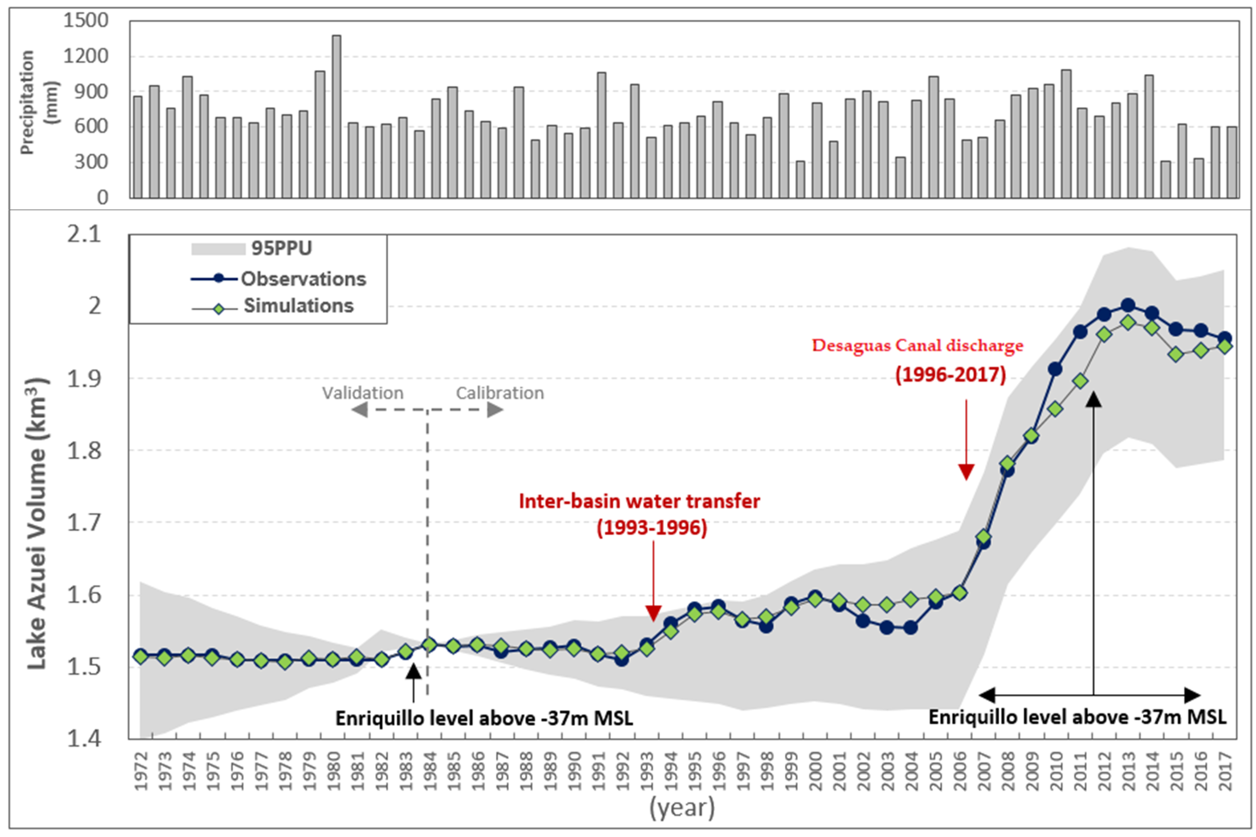
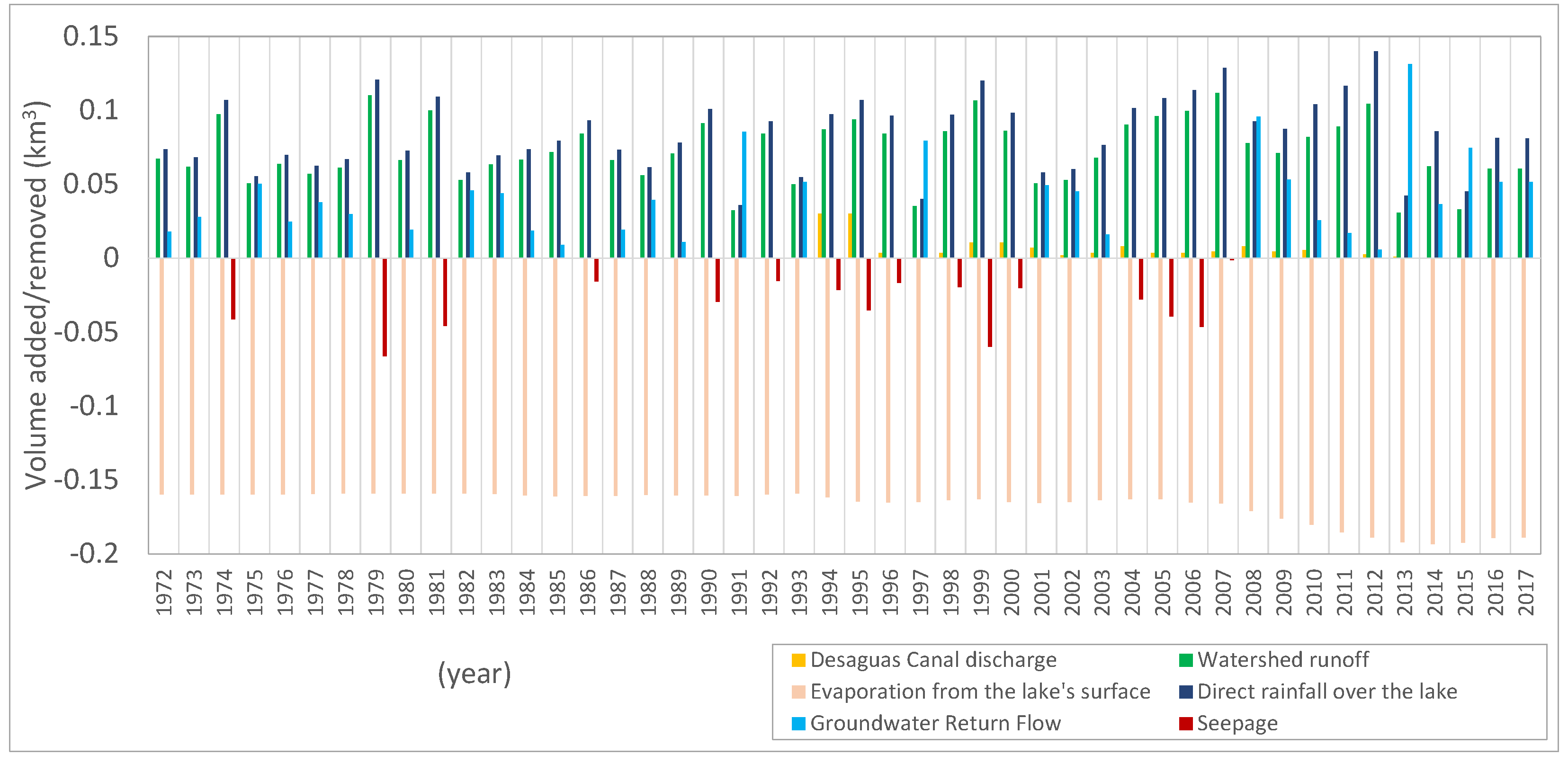
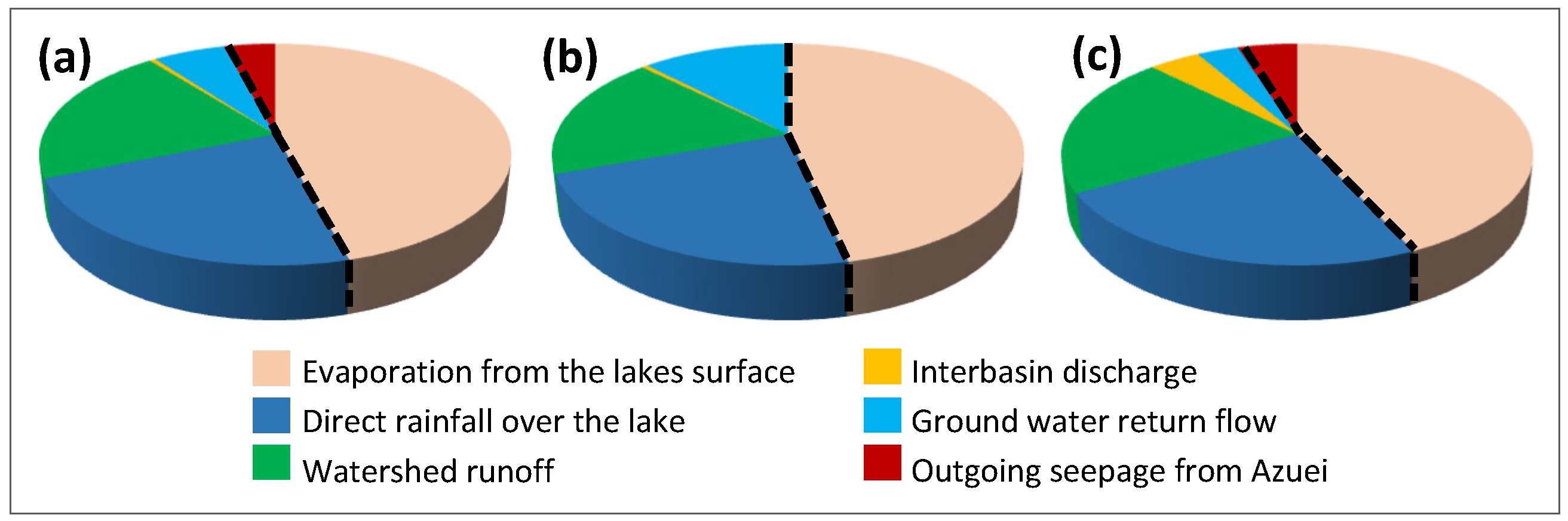
On average, the input flow to the LE system was composed of 49.1% direct rainfall, 31.1% watershed runoff, 14% Cristobal discharge, 2.6% groundwater return flow, and 3.2% inflow from LA. The primary and only output from the Enriquillo system was the lake surface evaporation. Although the annual contribution to LE’s volume is higher from direct rainfall than from runoff production, the lake’s sudden expansion is associated with the volume introduced from a storm event or through the Cristobal Canal. Therefore, it was concluded that LE and its watershed are more sensitive to storm events (caused by North Atlantic cyclone activities) and inter-basin water transfer. The least essential inputs of the LE water budget were groundwater return flow throughout years after a storm event (~0.01 km3/yr) and incoming seepage from LA (~0.02 km3/yr), which did not make any significant change in LE’s volume. It should be noted that, for the simulations, it was assumed that all LA seepage drains into LE. This might not be entirely true, with only tiny portions of the seepage entering LE.

3.1.2. Lake Azuei

Figure 10 depicts the LA volume time series along with volume simulations. This figure shows LA’s water budget’s two main external forces: (a) Inter-basin water transfer and (b) LE’s water level impact when it rises above −37 m MSL. As shown in Figure 10, the model shows satisfactory results in predicting the interannual behavior of the lake.
The main inputs of LA’s water budget were direct rainfall, surface runoff, groundwater return flow, and Desaguas Canal discharge. The main outputs were evaporation from the lake’s surface and groundwater outflow (outgoing seepage). Throughout the entire time series, the volume received by the lake from direct precipitation was higher than that of runoff, inter-basin water transfer discharge, and groundwater return flow (Figure 11). Additionally, the amount of evaporation was higher than the outgoing seepage from the lake’s system.
The eight sub-periods considered to characterize LA’s behavior are as follows:
1972–1982:
During this period, LA exhibited a stable behavior, and the amount of inflow and outflow to/from the lake was balanced. Average volumes estimated in this period were: 0.16 km3/yr due to evaporation, 0.08 km3/yr as direct rainfall, 0.07 km3/yr from runoff, 0.02 km3/yr via groundwater return flow, and 0.01 km3/yr as outgoing seepage from Azuei.
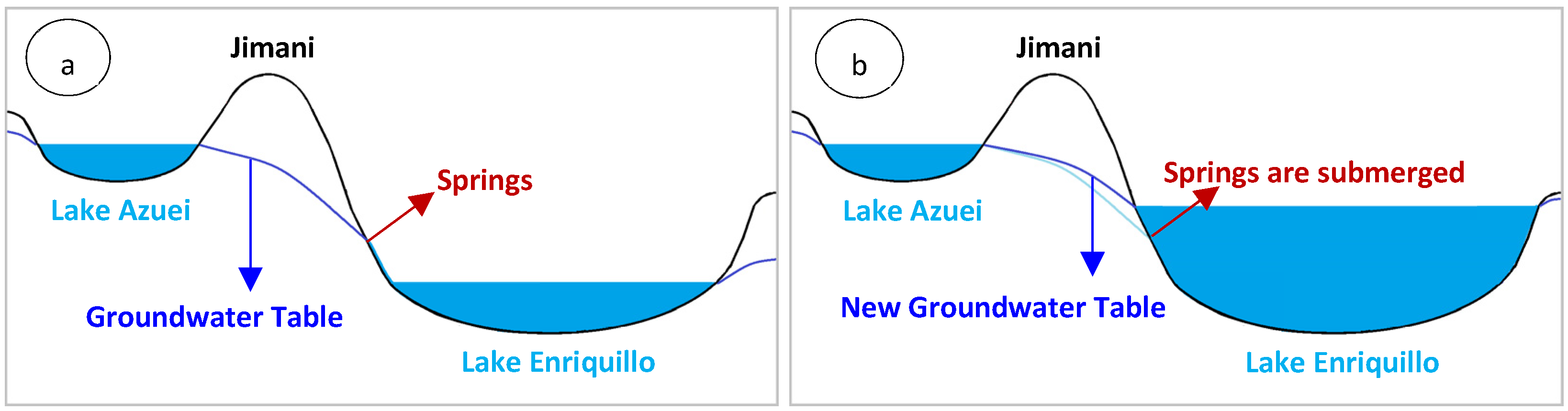
1983–1984:
During this short period, LA expanded slightly (~20 cm level rise) in response to LE’s level rising above –37 m MSL, which lasted for only a few years. For this period, groundwater return flow was approximately 0.03 km3/yr, while outgoing seepage was estimated to be close to zero, thus explaining the lake’s growth. Other elements of the water budget were: evaporation (~0.16 km3/yr), direct rainfall (~0.07 km3/yr), and runoff (~0.06 km3/yr).
1985–1992:
Soon after the expansion in 1982–1984, LA stabilized and attained its previous equilibrium, which was owed to removing LE’s influence. This period lasted for eight years, during which direct precipitation, runoff, groundwater return flow, and seepage values from Azuei were the same as the 1972–1982 period.
1993–1996:
A 5% expansion in the lake’s volume was observed, causing it to rise by 79 cm. This increase correlated with inter-basin water transfer without a significant precipitation event or LE’s influence. Based on water budget calculations, a total of 0.06 km3 had been added to the lake. Satellite imagery showed a possible water volume transfer from the Desaguas Canal to LA for 12 months during 1993 and 1996. To match the growth of LA, the Desaguas Canal would have had to supply 2.9 m3/s. The validity of this assumption would have to be investigated further.
1997–2000:
For these years, LA was experiencing stability. Based on satellite imagery, water budget estimations showed a discharge of 338 lit/s for 28 months. The values of water budget constituents were 0.16, 0.09, 0.08, 0.006, 0.02, and 0.02 km3/yr for evaporation, direct rainfall, runoff, Desaguas discharge, groundwater return flow, and outgoing seepage.
2001–2006:
Similar to LE observations, significant differences between observed and model simulations existed. These differences were attributed to the assumption of constant evaporation rate because those years coincided with a dry period. Satellite imagery showed 31 months of the Desaguas Canal flow (~0.005 km3/yr).
2007–2013:
LA’s surface-level rose by approximately 3.7 m in seven years. This synchronous expansion was a result of LE’s rapid surface level rise influencing Azuei’s system. Desaguas Canal flow continued to contribute to LA’s water budget for 29 months (~0.004 km3/yr). The water budget calculations showed an outgoing seepage value of close to zero from Azuei’s system. The calculation of other factors yielded: 0.18, 0.10, 0.08, and 0.05 km3/yr for evaporation, direct rainfall, runoff, and groundwater return flow, respectively. The higher rate of evaporation and direct rainfall was due to the significant expansion of the lake’s surface area. The discrepancies between simulations and observations for the years after 2009 are due to the inaccurate prediction of the equilibrium modifier, which changed during the rising leg of the time series. Assessments using the LA model showed that the lake would never have expanded if it were not for the influence of LE on its system.
2014–2017:
Synchronous with LE, LA was shrinking due to the gradual removal of LE’s impact on its dynamic. As mentioned before, the difference between simulations and observations was because of the simplifications applied to estimate the equilibrium modifier.
Generally, LA experienced more stable dynamics than LE. LA’s groundwater interactions (outgoing seepage and groundwater return flow) had an essential role in maintaining its water budget when no external force was present. To recap: when the rainfall amount during a specific year was less than the lake’s long-term rainfall, groundwater return flow stabilized its level and minimized the level drop. When the rainfall was higher than the lake’s long-term rainfall, lake water would seep into the groundwater layer, thus removing excess rainfall from the lake storage. However, LA’s stable condition changed when LE’s surface elevation rose above a certain level. During these years, the outgoing seepage was close to zero, and water budget analysis showed a high level of groundwater return flow into the lake.
For LA, water budget input contributions were as follow: 44.8% direct rainfall (~0.08 km3/yr), 38.9% watershed runoff (~0.07 km3/yr), 1.6% inter-basin discharge, and 14.7% groundwater return flow. The outflows of the Azuei water budget were 93.8% evaporation (~0.17 km3/yr) and 6.2% outgoing seepage. The average inter-basin water transfer value was estimated to be 0.008 km3/yr for the years it was present. Groundwater return flow to and outgoing seepage from the lake were estimated to be 0.019 and 0.017 km3/yr during the years with no influence from LE, and 0.04 and 0 km3/yr when LE’s external force was exerted on the LA’s system.

3.2. Lake Dynamics Description

Based on the information derived from the LE model, three distinct conditions can be identified for the LE system, each of which triggered different responses from the lake. On average (1972–2017), evaporation and direct rainfall account for 0.3 and 0.17 km3/yr, respectively. LE’s three responses are:
(a) When there is no storm activity in the region, and no discharge is coming from inter-basin sources (Cristobal Canal): Without these external forces, the lake cannot maintain its volume solely through direct rainfall over the lake runoff generated by everyday precipitation events. Simulations show that 3.5% of precipitation contributes to runoff generation across the watershed surface. Therefore, the lake shrinks inevitably due to the high evaporation rate (Figure 12a). This situation was observed in 1972–1978, 1982–1997, and 2000–2004. The average value of runoff estimated for these years was approximately 0.07 km3/yr.
(b) In the presence of impactful storms and hurricanes with no inter-basin water flows toward LE (Figure 12b): The lake’s rise of approximately 1 or 2 m in less than two years is expected due to the high production of runoff. During storm events, 12% of precipitation over the watershed contributes to runoff production. It takes approximately two years before the lake settles back to its previous size because of the gradual release of groundwater into the lake. An example of this is the occurrence of hurricane George in 1998 and storm Alpha in 2005. Water budget estimations show that runoff production tripled for those years (~0.2 km3/yr), and groundwater volume was 0.03 km3/yr.
(c) When impactful storm events and Cristobal Canal discharge are both present, they are the essential controls for the system: The volume of these two contributors plus direct rainfall, when added together, cancels out evaporation, increasing the lake’s volume (Figure 12c). A sudden rainstorm produces a higher amount of runoff (rc ~ 12%) than the years with the same cumulative precipitation value (rc ~ 3.5%). Conversely, Cristobal Canal discharge, which is triggered indirectly by storms on other watersheds, drains its excess water into LE, exacerbating the situation. Removal of both contributors causes the lake to recede gradually due to evaporation. This occurred between 1979–1980 and 2007–2014, for which the average volume added from runoff and Cristobal were 0.19 and 0.22 km3/yr, respectively.
While LA exhibits a more stable behavior, its water budget is susceptible to three conditions triggering three different responses:
(a) No external force is exerted on LA’s water budget by either the LE system or significant inter-basin water transfer: For this condition, the groundwater return flow compensates for the water needed to keep the lake stable for years with less precipitation. During years with high precipitation, groundwater outflow drains the extra water out of the system (Figure 13a).
(b) When LE influences LA (Figure 13b): LE surface levels affect Azuei’s groundwater table and subsequent subsurface flow exchanges between the lakes. This effect creates a simultaneous and synchronous behavior between the lakes as LA responds to LE’s system changes. Conceptualizing and quantifying this condition proved to be difficult due to the complexity of the hydrogeological dynamics involved. However, the regression formulation relating LE’s surface level to LA’s water budget produced acceptable and conclusive results through the initial assessment of the lakes’ systems. LA was experiencing such conditions in the periods 1980–1981 and 2007–2017. During the 2007–2014 period, The Desaguas Canal was active; however, its impact on the lake was insignificant due to its small discharge value.
(c) Significant inter-basin water input, whether LA is under the influence of LE’s system or not: This causes significant changes to the lake (Figure 13c). An example of this situation occurred in the period 1992–1996 when LA grew by 5%. During this time, LE had no impact on LA’s system, and the source of this flow has not yet been identified. No example is present to show when both LE and inter-basin water transfer factors are in effect. Therefore, the differentiation between the forcing signals of these two processes was not possible.

4. Conclusions

The modeling of LA and LE proved to be complex, given data scarcity and the many interactions between the lakes, their respective watersheds, and the hydroclimatic forcings. Much effort was spent collecting available data and generating and filling in the missing data to construct the time series needed to carry out analysis and modeling. The development of the watershed models involved extensive iterations between different model set-ups and model parametrizations to identify adequate formulations for representing the lakes and their water balance. The effort produced two distinct models for LE and LA that could be coupled when needed to represent the lake interactions.
For surface processes, a rainfall-runoff relationship proved adequate to model LA, and the assumption of constant runoff coefficient worked well for LA’s runoff characteristics. For LE, however, the runoff coefficient had to be adjusted for extreme precipitation events to account for the saturation of topsoil and, consequently, a high runoff production. For cases such as that, the optimized value of the runoff coefficient was increasing by more than three times its original value.
Quantifying groundwater flow around the lakes using physical approaches proved to be equally challenging due to the lack of hydrogeology studies in the region. Thus, groundwater flow was estimated using calculated precipitation rates. For LE, groundwater exchanges with the lake were assumed to be negligible for low-intensity precipitation events. After an impactful storm event, a fraction of precipitation that would infiltrate into the deep subsurface layer was added to the lake with exponentially decreasing rates to account for its observed growth in the years following the storm. For LA, an extra factor was introduced, named “equilibrium modifier,” into the groundwater equation to account for the stability of its system. In the absence of an external force (on the surface through inter-basin water transfer or on the subsurface exerted by LE), the equilibrium modifier was equal to the long-term average precipitation. Therefore, when rainfall was less than the long-term average, their difference would be added from groundwater storage to compensate for the water shortage in the system. When rainfall was higher than the average, the extra water would be removed from the system before reaching the lake in the form of outgoing seepage. The performance analysis of the model confirmed the appropriateness of the basic groundwater principles embodied in the models. However, formulations of groundwater flow such as the ones used for LE and LA have to be further investigated and applied to other closed-basin lakes with similar responses to internal and external drivers to see if they could be generalized to other groundwater modeling situations despite the scarcity of relevant data.
With LE being the lowest point in the study region, speculations suggested that LA’s growth was the reason behind the 2003–2014 growth of LE. However, the modeling results proved the opposite: (i) if LA were to impact LE, the expansion of LA in 1993–1996 had not impacted LE, and LE was constantly shrinking during that period; (ii) the 2003–2014 growth of LA started a few months after LE’s [29], and (iii) the contribution of subsurface fluxes (2.6% groundwater and 3.2% incoming seepage from LA) were insignificant when analyzing LE’s water budget. The “great” growth of LE is associated with the consecutive storm events in that period and the uncontrolled transfer of water from neighboring watersheds. Consequently, the hydrological systems of the lakes were (and are) connected, and the rise of LE resulted in the rise of LA. Moreover, it is essential to note that all outgoing seepage from the LA system was assumed to be entering LE’s. In reality, only a tiny portion of this seepage ends up in LE; hence the contribution of LA in LE’s water budget has to be less than the estimated values.
Overall, LE’s system has been shown to be alternating between prolonged shrinkages and sudden expansions, while LA stays steady as long as its system is not disturbed by any external factor. The results of this study are limited by the simplicity of the conceptual model and the assumptions made. However, these results lay a basis for future research to expand the knowledge of underlying processes identified through data gathering attempts and quantify them through comprehensive physical modeling.

Author Contributions

The authors have worked on various aspects of this manuscript, which is based on the doctoral work of M.M. More specifically, the various manuscript components have been addressed as follows: Conceptualization: M.M. and M.P.; methodology: M.M. and M.P.; validation: M.M.; formal analysis: M.M.; data curation: M.P. and M.M.; writing—initial draft: M.M.; writing—review and editing: M.P. and M.M.; visualization: M.M.; supervision: M.P.; project administration: M.P.; funding acquisition: M.P. All authors have read and agreed to the published version of the manuscript.

Funding

The authors would like to acknowledge the support for this study by the National Science Foundation (NSF) through grant 1264466 and the Department of Civil Engineering in the Grove School of Engineering at The City College of New York.

Institutional Review Board Statement

Not applicable.

Informed Consent Statement

Not applicable.

Data Availability Statement

The data underlying the analyses in this paper are available from the lead author Mahrokh Moknatian. The interested reader is encouraged to contact her using the email given in the header of this manuscript. Some data is also available from the CUNY Digital Library at: Moknatian M., Piasecki M., “Report: Observational Time Series for Lakes Azuei and Enriquillo: Surface Area, Volume, and Elevation”, New York, USA: Academic Works Digital Library, January 2019, https://academicworks.cuny.edu/cc_pubs/625/ (accessed on 12 August 2021).

Acknowledgments

We would like to extend our gratitude to our colleagues Naresh Devineni and Majid Heydari, who were instrumental in advising us on statistical analyses of time series.

Conflicts of Interest

The authors declare no conflict of interest. The funders had no role in the study design, in the collection, analyses, or interpretation of data, in the writing of the manuscript, or in the decision to publish the results.

References

  1. Mason, I.M.; Guzkowska, M.A.J.; Rapley, C.G.; Street-Perrott, F.A. The response of lake levels and areas to climatic change. Clim. Change 1994, 27, 161–197. [Google Scholar] [CrossRef]
  2. Shanahan, T.M.; Overpeck, J.T.; Sharp, W.E.; Scholz, C.A.; Arko, J.A. Simulating the response of a closed-basin lake to recent climate changes in tropical West Africa (Lake Bosumtwi, Ghana). Hydrol. Process. 2007, 21, 1678–1691. [Google Scholar] [CrossRef]
  3. Mercier, F. Interannual lake level fluctuations (1993–1999) in Africa from Topex/Poseidon: Connections with ocean–atmosphere interactions over the Indian Ocean. Glob. Planet. Change 2002, 32, 141–163. [Google Scholar] [CrossRef]
  4. Ricko, M.; Carton, J.A.; Birkett, C. Climatic effects on lake basins. Part I: Modeling tropical lake levels. J. Clim. 2011, 24, 2983–2999. [Google Scholar] [CrossRef] [Green Version]
  5. Mohammed, I.N.; Tarboton, D.G. An examination of the sensitivity of the Great Salt Lake to changes in inputs. Water Resour. Res. 2012, 48, 11. [Google Scholar] [CrossRef] [Green Version]
  6. Todhunter, P.E. Mean hydroclimatic and hydrological conditions during two climatic modes in the Devils Lake Basin, North Dakota (USA). Lakes Reserv. Res. Manag. 2016, 21, 338–350. [Google Scholar] [CrossRef] [Green Version]
  7. Troin, M.; Vallet-Coulomb, C.; Sylvestre, F.; Piovano, E. Hydrological modelling of a closed lake (Laguna Mar Chiquita, Argentina) in the context of 20th century climatic changes. J. Hydrol. 2010, 393, 233–244. [Google Scholar] [CrossRef]
  8. Moknatian, M.; Piasecki, M.; Gonzalez, J. Development of geospatial and temporal characteristics for Hispaniola’s Lake Azuei and Enriquillo using Landsat imagery. Remote Sens. 2017, 9, 510. [Google Scholar] [CrossRef] [Green Version]
  9. Jones, R.; McMahon, T.; Bowler, J. Modelling historical lake levels and recent climate change at three closed lakes, Western Victoria, Australia (c.1840–1990). J. Hydrol. 2001, 246, 159–180. [Google Scholar] [CrossRef]
  10. Phan, V.H.; Lindenbergh, R.C.; Menenti, M. Geometric dependency of Tibetan lakes on glacial runoff. Hydrol. Earth Syst. Sci. Discuss. 2013, 10, 729–768. [Google Scholar]
  11. Kaiser, K.; Heinrich, I.; Heine, I.; Natkhin, M.; Dannowski, R.; Lischeid, G.; Schneider, T.; Henkel, J.; Küster, M.; Heussner, K.-U.; et al. Multi-decadal lake-level dynamics in north-eastern Germany as derived by a combination of gauging, proxy-data and modelling. J. Hydrol. 2015, 529, 584–599. [Google Scholar] [CrossRef] [Green Version]
  12. Morrill, C.; Small, E.E.; Sloan, L.C. Modeling orbital forcing of lake level change: Lake Gosiute (Eocene), North America. Glob. Planet. Change 2001, 29, 57–76. [Google Scholar] [CrossRef]
  13. Todhunter, P.E.; Fietzek-DeVries, R. Natural hydroclimatic forcing of historical lake volume fluctuations at Devils Lake, North Dakota (USA). Nat. Hazards 2016, 81, 1515–1532. [Google Scholar] [CrossRef] [Green Version]
  14. Kebede, S.; Travi, Y.; Alemayehu, T.; Marc, V. Water balance of Lake Tana and its sensitivity to fluctuations in rainfall, Blue Nile basin, Ethiopia. J. Hydrol. 2006, 316, 233–247. [Google Scholar] [CrossRef]
  15. Huybers, K.; Rupper, S.; Roe, G.H. Response of closed basin lakes to interannual climate variability. Clim. Dyn. 2016, 46, 3709–3723. [Google Scholar] [CrossRef]
  16. Bracht-Flyr, B.; Istanbulluoglu, E.; Fritz, S. A hydro-climatological lake classification model and its evaluation using global data. J. Hydrol. 2013, 486, 376–383. [Google Scholar] [CrossRef] [Green Version]
  17. Zhou, J.; Wang, L.; Zhang, Y.; Guo, Y.; Li, X.; Liu, W. Exploring the water storage changes in the largest lake ( Selin Co) over the Tibetan Plateau during 2003–2012 from a basin--wide hydrological modeling. Water Resour. Res. 2015, 51, 8060–8086. [Google Scholar] [CrossRef] [Green Version]
  18. Langbein, W.B. Salinity and Hydrology of Closed Lakes; U.S. Geological Survey Professional Paper 412; U.S. Goverment Printing Office: Washington, DC, USA, 1961.
  19. Rosenberry, D.O.; Lewandowski, J.; Meinikmann, K.; Nützmann, G. Groundwater-the disregarded component in lake water and nutrient budgets. Part 1: Effects of groundwater on hydrology. Hydrol. Process. 2015, 29, 2895–2921. [Google Scholar] [CrossRef]
  20. Deus, D.; Gloaguen, R.; Krause, P. Water balance modeling in a semi-arid environment with limited in situ data using remote sensing in Lake Manyara, East African Rift, Tanzania. Remote Sens. 2013, 5, 1651–1680. [Google Scholar] [CrossRef] [Green Version]
  21. Turner, B.F.; Gardner, L.R.; Sharp, W.E. The hydrology of Lake Bosumtwi, a climate-sensitive lake in Ghana, West Africa. J. Hydrol. 1996, 183, 243–261. [Google Scholar] [CrossRef]
  22. Mohammed, I.N.; Tarboton, D.G. On the interaction between bathymetry and climate in the system dynamics and preferred levels of the Great Salt Lake. Water Resour. Res. 2011, 47, 1–15. [Google Scholar] [CrossRef] [Green Version]
  23. Clark, J.A.; Befus, K.M.; Sharman, G.R. A model of surface water hydrology of the Great Lakes, North America during the past 16,000 years. Phys. Chem. Earth 2012, 53–54, 61–71. [Google Scholar] [CrossRef]
  24. Vallet-Coulomb, C.; Legesse, D.; Gasse, F.; Travi, Y.; Chernet, T. Lake evaporation estimates in tropical Africa (Lake Ziway, Ethiopia). J. Hydrol. 2001, 245, 1–18. [Google Scholar] [CrossRef]
  25. Legesse, D.; Vallet-Coulomb, C.; Gasse, F. Analysis of the hydrological response of a tropical terminal lake, Lake Abiyata(Main Ethiopian Rift Valley) to changes in climate and human activities. Hydrol. Process. 2004, 18, 487–504. [Google Scholar] [CrossRef]
  26. Scheffers, A.; Browne, T. Encyclopedia of the World’s Coastal Landforms: Hispaniola (Haiti and the Dominican Republic); Bird, E.C.F., Ed.; Springer: Dordrecht, The Netherlands, 2010; Volume 2, pp. 7–10. ISBN 978-1-4020-8638-0. [Google Scholar]
  27. Moknatian, M.; Piasecki, M.; Moshary, F.; Gonzalez, J. Development of digital bathymetry maps for Lakes Azuei and Enriquillo using sonar and remote sensing techniques. Trans. GIS 2019, 23, 841–859. [Google Scholar] [CrossRef] [Green Version]
  28. Moknatian, M.; Piasecki, M. Observational Time Series for Lakes Azuei and Enriquillo: Surface Area, Volume, and Elevation; Research Report; CUNY Academic Works: New York, NY, USA, 2019. [Google Scholar]
  29. Moknatian, M.; Piasecki, M. Lake Volume Data Analyses: A Deep Look into the Shrinking and Expansion Patterns of Lakes Azuei and Enriquillo, Hispaniola. Hydrology 2019, 7, 1. [Google Scholar] [CrossRef] [Green Version]
  30. González, R.; Brito, D.R.; González, J. Estudio Hidrogeológico de la Zona del Lago Enriquillo, Determinación de las Causas del Aumento de Nivel de Sus Aguas e Intervenciones Requeridas Para su Control; Project Progress Report NO.1; Instituto Tecnológico de Santo Domingo (INTEC) and the City College of New York (CCNY): New York, NY, USA, 2010. [Google Scholar]
  31. Vlaminck, B. La Pecherie de L’etang Saumatre: Recherche Appliquee et Activites Periode Octobre 88–Septembre 89; Project Report HAI/88/003; United Nations Development Programme/Food and Agriculture Organization (PNUD/FAO): Haiti, Indonesia, 1989. [Google Scholar]
  32. Perrissol, M.; Lescoulier, C. Etude Hydrologique et Hydrogéologique de la Montée des eaux du lac Azueï; Project Repor; Version 2; Egis International: Haiti, Indonesia, 2011. [Google Scholar]
  33. Buck, D.G.; Brenner, M.; Hodell, D.A.; Curtis, J.H.; Martin, J.B.; Pagani, M. Physical and chemical properties of hypersaline Lago Enriquillo, Dominican Republic. SIL Proc. 2005, 29, 725–731. [Google Scholar] [CrossRef]
  34. Pichardo, F.D.G.; Conte, L.L.; Regio, G. Alternativas Productivas a Mediano y Largo Plazo Para las Familias Afectadas por la Crecida del Nivel del Lago Enriquillo; Project Report prepared by OXFAM-Italy; OXFAM-Italy: Santo Domingo, Dominican Republic, 2012. [Google Scholar]
  35. Martínez-Batlle, J.R. Sierra de Bahoruco Occidental, República Dominicana: Estudio Biogeomorfológico y Estado de Conservación de su Parque Nacional. Ph.D. Thesis, Departamento de Geografía Física y Análisis Geográfico Regional, Universidad de Sevilla, Sevilla, Spain, 2012. [Google Scholar]
  36. Gilboa, Y. The aquifer systems of the Dominican Republic. Hydrol. Sci. Bull. 1980, 25, 379–393. [Google Scholar] [CrossRef]
  37. Schubert, A. El Lago Enriquillo: Gran Patrimonio Natural y Cultural del Caribe, 2nd ed.; Secretaría de Medio Ambiente y Recursos Naturales Consorcio Ambiental Dominicano CAD: Jimani, Dominican Republic, 2003; ISBN 99934-0-110-2. [Google Scholar]
  38. Mendez-Tejeda, R.; Delanoy, R.A. Influence of climatic phenomena on sedimentation and increase of Lake Enriquillo in Dominican Republic, 1900–2014. J. Geogr. Geol. 2017, 9, 19. [Google Scholar] [CrossRef]
  39. Méndez-tejeda, R.; Rosado, G.; Rivas, D.V.; Montilla, T.; Hernández, S.; Ortiz, A.; Santos, F. Climate variability and its effects on the increased level of Lake Enriquillo in the Dominican Republic, 2000–2013. Appl. Ecol. Environ. Sci. 2016, 4, 26–36. [Google Scholar]
  40. Logan, W.S.; Enfield, D.B.; Division, P.O.; Capdevila, A.S. Rising Water Levels at Lake Enriquillo, Dominican Republic: Advice on Potential Causes and Pathways forward. Report by the International Center for Integrated Water Resources Management (ICIWaRM) to the Instituto Nacional de Recursos Hidráulicos (INDRHI), Government of the Dominican Republic. 2012. Available online: https://s3.amazonaws.com/sitesusa/wp-content/uploads/sites/422/2015/12/Lake_Enriquillo_report_1-26-2012.pdf (accessed on 12 August 2021).
  41. Araguás Araguás, L.; Mchelen, C.; Garcia, A.; Medina, J.; Febrillet, J. Estudio de la Dinamica del Lago Enriquillo: Segundo Informe de Avance; Project Report DOM/8/006; International Atomic Energy Agency: Vienna, Austria, 1995. [Google Scholar]
  42. Arboleda, J. Independencia: Perfil Socio-Economico y Medioambiental; Programa de las Naciones Unidas para el Desarrollo (PNUD): Santo Domingo, Dominican Republic, 2013; ISBN 978-9945-8741-4-3. [Google Scholar]
  43. Programa de Naciones Unidas para el Desarrollo (PNUD). Plan Estratégico de Recuperación y Transición al Desarrollo Para la Zona del Lago Enriquillo; Editora Búho, Proyecto Frontera-UNDP: Santo Domingo, Dominican Republic, 2013. [Google Scholar]
  44. Mejía, V.A.M.; León, Y.; Quintana, C.; Rosario, A. Contribution of surface water sources in the eastern part of Lake Enriquillo and the impact of these waters to the growth of the lake. Cienc. Soc. 2015, 40, 425–448. [Google Scholar]
  45. Quezada, A.C. El ciclo Hidrologico del Lago Enriquillo y la Crecida Extrema del 2009; Report available at Acqweather.com; Acqweather: Santo Domingo, Dominican Republic, 2009. [Google Scholar]
  46. Ducoudray, F.S. Dominican Nature, Article Published in the Saturday Supplement of the Newspaper El Caribe (1978–1989); Southern, R., Ed.; Aristides Inchaustegui, Blanca Delgado Malagón; Grupo León Jiménez: Santo Domingo, Dominican Republic, 2006; Volume 2, pp. 273–274. [Google Scholar]
  47. Sheller, M.; León, Y.M. Uneven socio-ecologies of Hispaniola: Asymmetric capabilities for climate adaptation in Haiti and the Dominican Republic. Geoforum 2016, 73, 32–46. [Google Scholar] [CrossRef]
  48. Piasecki, M.; Moknatian, M.; Moshary, F.; Cleto, J.; Leon, Y.; Gonzalez, J.; Comarazamy, D. Bathymetric Survey for Lakes Azuei and Enriquillo, Hispaniola; Research Report; CUNY Academic Works: New York, NY, USA, 2016. [Google Scholar]
  49. Dale, V.H.; Beyeler, S.C. Challenges in the development and use of ecological indicators. Ecol. Indic. 2001, 1, 3–10. [Google Scholar] [CrossRef] [Green Version]
  50. Patrício, J.; Neto, J.M.; Teixeira, H.; Salas, F.; Marques, J.C. The robustness of ecological indicators to detect long-term changes in the macrobenthos of estuarine systems. Mar. Environ. Res. 2009, 68, 25–36. [Google Scholar] [CrossRef] [Green Version]
  51. Choubak, M.; Pereira, R.; Sawatzky, A. Indicators of Ecological Behaviour Change; Community Engaged Scholarship Institute: Guelph, ON, Canada, 2019. [Google Scholar]
  52. Harmsen, E.W. Puerto Rico Agricultural Water Management (PEAGWATER). Available online: https://pragwater.com/ (accessed on 18 February 2018).
  53. Szesztay, K. Water balance and water level fluctuations of lakes. Hydrol. Sci. 1974, 19, 73–84. [Google Scholar] [CrossRef]
  54. Izzo, M.; Aucelli, P.P.C.; Javier, Y.; Pérez, C.; Rosskopf, C.M. The tropical storm Noel and its effects on the territory of the Dominican Republic. Nat. Hazards 2010, 53, 139–158. [Google Scholar] [CrossRef]
  55. Kieniewicz, J.M.; Smith, J.R. Paleoenvironmental reconstruction and water balance of a mid-Pleistocene pluvial lake, Dakhleh Oasis, Egypt. GSA Bull. 2009, 121, 1154–1171. [Google Scholar] [CrossRef]
  56. Eptisa Internacional Grupo EP. Unidad Hidrogeológica de la Sierra de Bahoruco y Península Sur de Barahona; Informe de la Estudio Hidrogeológico Nacional de la República Dominicana Fase II.; Santo Domingo, Dominican Republic, 2004; Available online: https://gymrd.com/hidro/estudio/Estudio%20Hidrogeol%C3%B3gico%20de%20la%20Sierra%20de%20Bahoruco%20y%20Pen%C3%ADnsula%20Sur%20de%20Barahona.pdf (accessed on 12 August 2021).
  57. Smucker, G.R.; Bannister, M.; D’Agnes, H.; Gossin, Y.; Portnof, M.; Timyan, J.; Tobias, S.; Toussaint, R. Environmental Vulnerability in Haiti: Findings & Recommendations; Report prepared by Chemonics International Inc. and the U.S. Forest Service for for review by the United States Agency for International Development (USAID); USAID: Haiti, Indonesia, 2007.
  58. International Resources Group Ltd. Dominican Republic Environmental Assessment; Report prepared for the United States Agency for International Development (USAID); United States Agency for International Development (USAID): Santo Domingo, Domonican Republic, 2001.
  59. Versluis, A.; Rogan, J. Mapping land-cover change in a Haitian watershed using a combined spectral mixture analysis and classification tree procedure. Geocarto Int. 2010, 25, 85–103. [Google Scholar] [CrossRef]
  60. Mora, S.; Roumagnac, A.; Asté, J.-P.; Calais, E.; Haase, J.; Saborío, J.; Marcello, M.; Milcé, J.-E.; Zahibo, N. Analysis of Multiple Natural Hazards in Haiti; Report prepared by the Government of Haiti, with support from the World Bank, the Inter-American Development Bank, and the United Nations System; Government of Haiti: Port-au-Prince, Haiti, 2010. [Google Scholar]
  61. Emmanuel, E. Atelier sur la Gestion et la Legislation de l’Eau, Haiti; Pre-Workshop Report; Technical cooperation BID No. ATN/SF-5485-HA, Programme de Formulation de la Politique de l’Eau; Ministère de l’Environnement: Port-au-Prince, Haiti, 1998. [Google Scholar]
  62. Abbaspour, K.C.; Johnson, C.A.; van Genuchten, M.T. Estimating uncertain flow and transport parameters using a sequential uncertainty fitting procedure. Vadose Zo. 2004, 3, 1340–1352. [Google Scholar] [CrossRef]
  63. Moriasi, D.N.; Arnold, J.G.; Van Liew, M.W.; Bingner, R.L.; Harmel, R.D.; Veith, T.L. Model evaluation guidelines for systematic quantification of accuracy in watershed simulations. Trans. ASABE 2007, 50, 885–900. [Google Scholar] [CrossRef]
Figure 1. Study area watershed system (green boundaries show the watersheds’ extent; deep red lines are canals delineated using google earth; the arrows demonstrate the direction of water transfer in the canals).
Hydrology 08 00148 g001
Figure 2. Interannual volume time series of Lake Azuei and Lake Enriquillo (data for 1996–2014 are derived from monthly time series. Data for 1972–1995 and 2014–2017 are estimations derived from Landsat imagery).
Hydrology 08 00148 g002
Figure 3. Schematic location of groundwater table: (a) Lake Enriquillo’s water level is below the springs’ location, (b) Lake Enriquillo’s water level is above the springs’ location.
Hydrology 08 00148 g003
Figure 4. Lake Enriquillo model parameter frequency distribution of runoff coefficients (rc1 and rc2) and inter-basin water transfer volume (Q) obtained using Monte Carlo method.
Hydrology 08 00148 g004
Figure 5. Simulated vs. observed volume and volume change values of Lake Enriquillo for calibration and validation periods.
Hydrology 08 00148 g005
Figure 6. Lake Azuei model parameter frequency distribution of runoff coefficient (rc) and inter-basin water transfer in form discharge (Q) obtained using Monte Carlo method.
Hydrology 08 00148 g006
Figure 7. Simulated vs. observed volume and volume change values of Lake Azuei for calibration and validation periods.
Hydrology 08 00148 g007
Figure 8. Lake Enriquillo’s observed and simulated volume time series and the two major external forces exerted on the lake’s system.
Hydrology 08 00148 g008
Figure 9. Enriquillo’s water budget component time series.
Hydrology 08 00148 g009
Figure 10. Lake Azuei’s observed and estimated volume time series and the two major external forces exerted on the lake’s system.
Hydrology 08 00148 g010
Figure 11. LA time series for water budget components.
Hydrology 08 00148 g011
Figure 12. Water balance component proportions for Lake Enriquillo’s dynamics phases: (a) Shrinkage pattern when no storm incident and no inter-basin water transfer are present; (b) Expansion pattern when only storm incident is present; and (c) Expansion pattern when storm incident and inter-basin water transfer are both present (Black dashed line separates inflows and outflows to/from the lake).
Hydrology 08 00148 g012
Figure 13. Water balance component proportions for Lake Azuei’s dynamics phases: (a) Steady-state when no external force is present; (b) Expansion pattern when the influence of Lake Enriquillo is present; and (c) Lesser expansion pattern when significant inter-basin water transfer is present (Black dashed line separates inflows and outflows to/from the lake).
Hydrology 08 00148 g013
Table 1. Enriquillo model’s calibration and validation performance and uncertainty analysis.
NSERSSRMSEMAEREp-factorr-factor
CalibrationVolume Change0.780.2760.0910.074−9.2%33%0.41
Volume 0.970.6620.1420.1220.9%94%0.92
ValidationVolume Change0.580.1300.1040.08516.7%50%0.66
Volume 0.920.0620.0720.0843.1%92%1.78
Table 2. Azuei model’s calibration and validation performance and uncertainty analysis.
NSERSSRMSEMAEREp-factorr-factor
CalibrationVolume Change0.710.00650.01410.011−14%45%0.59
Volume 0.990.00730.01490.015−0.18%100%0.97
ValidationVolume Change0.638.92 × 10−50.002620.00212%83%5.54
Volume 0.875.52 × 10−50.002060.0020.01%83%2.51
Table 3. Water budget parameter values and ranges for LE and LA between 1972 and 2017.
ParameterLake EnriquilloLake Azuei
V t (km3/yr) *Lake volume change time series [–0.39, +0.75] **Lake volume change time series [–0.02, +0.1]
A L (km2) *Lake surface area time series [168.1, 349.6]Lake surface area time series [113.7, 138.1]
A w (km2) * 3062.3 A L 805 A L
P L (mm/yr)Jimani station annual records [306, 1084]Jimani station annual records [306, 1084]
P w (mm/yr) 1.07 × P L 1.37 × P L
E L (mm/yr)12501400
P ¯ w (mm/yr)not applicable733 or f (LE’s elev)
i n f c 0.190.21
r c   *** [0, 0.6][0, 0.6]
f 0 or 1[0, 1]
Q     *** (m3/s) *[0, 25]No range is available
G L A (mm/yr) The   absolute   value   of   ( i n f c ( P ¯ w P w ) A w ) term from LA’s water budget when it is negativenot applicable
* Units are converted from km and m to mm in the water budget calculations. ** Observed/considered upper and lower values. *** The parameter value is optimized through the calibration process.
Publisher’s Note: MDPI stays neutral with regard to jurisdictional claims in published maps and institutional affiliations.

