
Characteristics of Internal Tides from ECCO Salinity Estimates and Observations in the Bay of Bengal

1
School of the Earth, Ocean and Environment, University of South Carolina, Columbia, SC 29208, USA
2
Physical Oceanography Division, Council of Scientific and Industrial Research (CSIR)—National Institute of Oceanography (NIO), Regional Centre, Visakhapatnam 530017, India
*
Author to whom correspondence should be addressed.
Remote Sens. 2023, 15(14), 3474; https://doi.org/10.3390/rs15143474
Submission received: 19 May 2023
/
Revised: 30 June 2023
/
Accepted: 2 July 2023
/
Published: 10 July 2023
(This article belongs to the Special Issue Advances in Remote Sensing of Ocean Salinity)
Abstract
:Internal waves (IWs) are generated in all the oceans, and their amplitudes are large, especially in regions that receive a large amount of freshwater from nearby rivers, which promote highly stratified waters. When barotropic tides encounter regions of shallow bottom-topography, internal tides (known as IWs of the tidal period) are generated and propagated along the pycnocline due to halocline or thermocline. In the North Indian Ocean, the Bay of Bengal (BoB) and the Andaman Sea receive a large volume of freshwater from major rivers and net precipitation during the summer monsoon. This study addresses the characteristics of internal tides in the BoB and Andaman Sea using NASA’s Estimating the Circulation and Climate of the Ocean (ECCO) project’s high-resolution (1/48° and hourly) salinity estimates at 1 m depth (hereafter written as ECCO salinity) during September 2011–October 2012, time series of temperature, and salinity profiles from moored buoys. A comparison is made between ECCO salinity and NASA’s Soil Moisture Active Passive (SMAP) salinity and Aquarius salinity. The time series of ECCO salinity and observed salinity are subjected to bandpass filtering with an 11–14 h period and 22–26 h period to detect and estimate the characteristics of semi-diurnal and diurnal period internal tides. Our analysis reveals that the ECCO salinity captured well the surface imprints of diurnal period internal tide propagating through shallow pycnocline (~50 m depth) due to halocline, and the latter suppresses the impact of semi-diurnal period internal tide propagating at thermocline (~100 m depth) reaching the sea surface. The semi-diurnal (diurnal) period internal tides have their wavelengths and phase speeds increased (decreased) from the central Andaman Sea to the Sri Lanka coast. Propagation of diurnal period internal tide is dominant in the northern BoB and northern Andaman Sea.
1. Introduction
Internal waves (IWs) are ubiquitous throughout the global oceans, existing well below the ocean’s surface at the interface separating different density layers (i.e., the pycnocline) and the ambient stratification, thus plays a key role in the energetics of IWs [1]. An external disturbance, such as shallow bathymetry, can disrupt barotropic tides resulting in the oscillating pattern of an IW. The oscillation frequency of internal tides is set by the frequency of the forcing [2]. Eventually, IW energy dissipates into turbulent mixing due to their breaking in the stratified ocean [3].
The Indian Ocean is known for its monsoonal wind reversals and surface currents, which govern the net precipitation and continental runoff that predominantly flows into the Bay of Bengal (BoB) and the Andaman Sea. The addition of freshwater to the ocean enhances local stratification between the freshwater surface layer and the dense, saline water layer below. There are two primary monsoon seasons in the Indian Ocean, the Southwest (SW) monsoon (June–September) and the Northeast (NE) monsoon (November–February), where the former is deemed as the wetter season with strong surface winds. The SW monsoon brings in large continental precipitation resulting in an accumulation of river discharge into the northern BoB and northern Andaman Sea coastal regions [4]. In the southern BoB, positive wind stress curls from the high wind speeds prompt the mixing of more saline Arabian Sea and equatorial water with the fresh water from the BoB area [5]. Wind forcing also controls the advection of freshwater plumes that influence the propagation and dissipation of IWs. Therefore, both the magnitude of freshwater discharge and wind stress are important factors towards favorable conditions of energetic IWs [6]. The vast spatial differences in freshwater distribution and magnitude throughout the BoB (Figure 1), especially through different monsoonal seasons, make it exceptionally important to observe the salinity-dominated component when identifying IWs.
As Phaniharam et al. [7] studied the IW characteristics in the northwestern BoB in a box (18–20°N and 85–86°E) using the synthetic aperture radar (SAR) data and in situ, observations and estimated their propagation phase speed of 0.12 to 0.5 m/s with an estimated amplitude of 8 m. These authors noted that the IWs in this region are generated due to the stratified layers disturbed by the tidal forces, and the stratification is resulted due to freshwater discharge from major rivers. In the northern BoB, strong stratification prevails at the end of the SW monsoon and a weaker stratification prior to the SW monsoon (March–May) [8,9]. Madhu et al. [10] studied the generation and propagation of IWs in the shelf waters of the western BoB from observations and using the Massachusetts Institute of Technology (MIT) general circulation model (MITgcm) forced with astronomical tides and daily winds for winter 2012 and identified the zones of sources/sinks for the generation of internal tides in the northwestern BoB to lie along the isobaths (500 m and 1500 m). These authors reported the phase speed of internal tides as 0.75 m/s in the open sea waters and 0.45 m/s on the shelf waters from Envisat SAR imagery in February 2012. The MIT model simulated the phase speed of the barotropic internal tides, which varied from 3 m/s in deep waters to 1 m/s in shallow waters.
The Andaman Sea is a prominent IW-generating region that is characterized by shallow bathymetry of the Andaman–Nicobar Island chain and the bordering continental shelves. Here, IWs are predominantly influenced by semi-diurnal tides, especially mode-2-tides, with IW packets occurring every 12.4 h [11,12,13]. From mooring observations in the southern Andaman Sea, Osborne et al. [14] show that the semi-diurnal tidal period IWs are of higher amplitude (60–80 m) and higher (1.8 m/s) surface current speed. Observations of large amplitude (82 m) IWs were reported off the northwestern coast of Sumatra [15] from the analysis of bathythermograph records. IWs can be seen throughout the year in the Andaman Sea and BoB but show peak amplitudes in April and November [16,17]. Apel et al. [18] found that around 70% of barotropic energy from barotropic tides was converted to baroclinic energy in the Andaman Sea, where roughly 30% is emitted out of the generation area in the Andaman Sea.
IWs usually result from barotropic tides, which flow over bottom topography, causing density oscillations to propagate along the pycnocline with a tidal frequency (i.e., internal tides). The large-scale waves propagate from the generation location and disintegrate into non-linear, short-scale, high-frequency IW packets. These short-scale IWs in the ocean are associated with the vertical structures in the water column of the lowest fundamental mode. Whereas higher, vertical modes are short-lived. Short-scale mode-2 IWs are documented in the Andaman Sea. Satellite-based SAR imageries have been used to detect surface roughness signals from the reverberating effects of IWs [1,18]. The crests and troughs associated with mode-1 (first baroclinic mode) IWs traveling along the pycnocline can create zones of divergence and convergence patterns at the ocean surface [19]. The convergence (divergence) of water parcels from the activity of IWs produces a rough (smooth) sea surface.
Sunglint, true ocean color images of Chlorophyll-a concentrations have also been used for IW detection as dense ocean color signifies IWs with large heights [16]. Wijeratne et al. [17] noticed that IWs originated in the Andaman Sea and propagated to the Sri Lanka coast in about 6–8 days. Several studies using satellites and in situ observations reveal different generation sites in the Andaman Sea [20,21,22]. Magalhaes and Da Silva [22] showed that both mode-1 and mode-2 internal solitary waves (or solitons) are present in the Ten Degree channel in the Andaman Sea and propagate towards the east. Raju et al. [23] studied the potential generation of large-scale, tidally generated IWs of mode-1 vertical structure (i.e., internal solitary waves) in the Andaman Sea using remote sensing observations of modern-resolution imaging spectroradiometer (MODIS) true-color images and SAR observations and identified five generating sites of internal solitary waves. Internal solitary waves generated at the western Nicobar Islands propagate westward into the BoB, and those generated in the Great Channel (or Sixth Degree Channel) of the southern Andaman Sea propagate towards the Thailand coast. Da Silva and Magalhaes [24] reported the generation of mode-2 internal solitary waves in the Andaman Sea in association with the double maxima in the profiles of buoyancy frequency. Hyder et al. [25] found the IWs in the northwest Andaman Sea occurred only during spring tides when the tidal range exceeds 1.5 m. Long-lived, solitary waves propagating along the Ten Degree Channel were reported to have mode-2 IW phase speeds around 0.6–0.7 m/s for depths greater than 1000 m [22,26]. In the Ten Degree Channel, mode-2 solitary waves are observed most of the year.
However, numerical investigations and SAR images identified the mode-1 and mode-2 IWs generated at the Batti Mav Island of the Car–Nicobar Island chain and explained the mechanisms for their generation [27]. They noticed that the mode-1 IW is generated at 80 m depth, where the model simulated Brunt-Väisälä frequency is maximum, with strong surface signatures. In another study by Tensubam et al. [28], the authors identified four regions of internal solitary wave generation in the Andaman Sea such as the northern Andaman Sea, the central-eastern Andaman Sea, around the Nicobar Islands, and the southeastern region near Sumatra from SAR images and Sunglint optical images of MODIS, visible infrared imaging radiometer suite (VIIRS) and medium resolution imaging spectrometer (MERIS). In SAR images, the mode-1 internal solitary waves are visible as patterns of bright bands followed by dark bands, while in Sunglint optical images, the same is seen as patterns of dark bands followed by bright bands. The sea surface roughness enhances in the convergence zones where the IW amplitude is large and decreases in the divergence zones where the amplitude is smaller.
Using the satellite altimeter-derived sea surface height (SSH) data and the simulations from the Regional Ocean Modelling System (ROMS) of the high-resolution (1/48°) ocean circulation model, as described in [29]. Jithin et al. [30] studied the spatial variability of internal tides in the BoB. Susanto and Ray et al. [31] studied seasonal and interannual variability of tidal mixing signatures in Indonesian Seas from NASA’s Multi-Scale Ultra-High Resolution (MUR) seas surface temperature product.
IWs pose a threat to subsurface environments as their energy propagations encounter commercial oil rigs. They can also affect the local environment by redistributing nutrients through mixing, and the resulting fluctuation of density gradients can interfere with underwater acoustics from submarines or from migratory species such as whales. Therefore, there is a necessity to enhance the robustness of our methodology of IW detection and characterization. There is not much information pertaining to the use of salinity data to determine surface signals or imprints of IWs and delineate their characteristics, even though this density-driven phenomenon fundamentally relies on the differences in salinity fluctuations in the BoB. Therefore, our analysis in this study encompasses both the generation region in the Andaman Sea and the paths of their propagation towards the northwestern and southwestern BoB. This work provides, possibly, the first-time detection of IWs in this region and their propagation into the BoB by analyzing salinity from a high-resolution ocean model simulation.
The objective of the present study is to use the surface salinity estimates from NASA’s Estimating the Circulation and Climate of the Ocean (ECCO) high-resolution (1/48°) simulations to detect IWs and define their characteristics in the Andaman Sea, known for the generation of large IWs, and their propagation into the BoB (Figure 1). ECCO estimates are compared to in situ moored buoy measurements [32,33] and satellite observations as well to detail their accuracy. Profiles of temperature, density, and the Brunt–Väisälä frequency are described as they can tell us more about the subsurface structure of IWs. The study period is focused on between November 2011 and October 2012 to match the period of the high-resolution release of the ECCO salinity estimates.
This study is to understand the propagating characteristics of the IWs in the Andaman Sea and BoB. We selected a total of two boxes in the Andaman Sea and four boxes in the BoB (Figure 1). In the proper Andaman Sea, one box (box A) is in the central Andaman Sea, and the other box (box D) is in the northern Andaman Sea. The basis for the selection of boxes in the BoB is the study of Jensen et al. [16] on the IWs using the SSH anomalies data and model simulations and the study of Jithin et al. [30] on the spatial variability of internal tides in the BoB. Jensen et al. [16] have shown that the IWs generated in the Andaman Sea propagate in a southwesterly direction from the Ten Degree Channel region towards Sri Lanka and south of Sri Lanka. Accordingly, we have selected one box (box B) off the western Car-Nicobar Islands covering the Ten Degree Channel and one box (box C) off Sri Lanka. Jensen et al. [16] have also reported the northwestward propagation of IWs from the northern Andaman Sea up to northwestern BoB. Accordingly, we have selected one more box (box E) off the northwestern Andaman Islands and another box (box F) in the northwestern BoB. Using the satellite altimeter-derived SSH data and the simulations from the Regional Ocean Modelling System (ROMS) of high resolution (1/48°) ocean circulation model, as described in [29,30] studied the spatial variability of internal tides in the BoB. These authors reported the existence of three major internal tide generation sites—the northwest coast of Andaman Islands covering the Preparis Channel, northeastern BoB, and northwestern BoB on the continental shelf edges. They reported that the total energy flux associated with the mode-2 internal tide is predominantly radiated towards north-central BoB from these sites. Our selected box F domain lies within the southward radiation of total energy flux from the northwestern BoB site, and the region of concentration of total energy flux in the north-central BoB occurs with the box E domain from the internal tide generation sites of Preparis Channel and northeastern BoB. Thus, the selected boxes E and F cover a larger portion of the prominent southward and westward radiation of total energy and its enhancement into the north-central BoB.
Our main aim in this study is to obtain the characteristics of internal waves of the tidal period and their propagation directions across the BoB from the Andaman Sea from the high-resolution ECCO salinity estimates and moored buoy observations. This study details the data, model estimates, and methodology in Section 2; the results are presented in Section 3, and the discussion is provided in Section 4, and the conclusions of the study are given in Section 5.
2. Data and Methods
2.1. Estimating the Circulation and Climate of the Ocean (ECCO) Salinity Estimates
This study uses hourly salinity data at 1 m depth from NASA’s ECCO (https://ecco-group.org (accessed on 29 March 2021)) project’s 1/48° (2.3 km) Massachusetts Institute of Technology general circulation model (MITgcm; https://mitgcm.org (accessed on 29 March 2021)) simulation LLC4320 and is available through https://data.nas.nasa.gov/ecco/data.php (accessed on 29 March 2021). The simulation LLC4320 denotes the Latitude-Longitude polar Cap (LLC) grid that is used with a 4320 resolution along each common face direction (i.e., 4320 points taken every 90° at this resolution; [34,35]). In this case, the grid size maximizes the number of integer factors for coarsening the grid and efficiently partitioning the computational domain [34]. Six-hourly European Centre for Medium-Range Weather Forecasts (ECMWF) ERA-Interim reanalysis fields (ERA-5 fields were not available when these simulations were performed) are also incorporated to compute surface fluxes (evaporation, precipitation, humidity; [35,36]) river runoff uses a seasonal climatology from [37], and barotropic tides [38,39]. This modified version of ECCO includes exchanges between the surface of the ocean and the atmospheric boundary layer, land, and sea ice compared to its previous version. The temporal period of this study is based on this version of ECCO, with hourly 1/48° resolution, which was run between 1 November 2011 and 31 October 2012 as a precursor for NASA Surface Water Topography Mission (SWOT) mission, which was launched on 16 December 2022. The resolutions of these estimates can resolve internal tides and sub-mesoscale structures and internal gravity waves associated with this study [25].
2.2. Observations
Wind velocities are obtained from NOAA’s Blended Sea Winds dataset, which are generated by synthesizing observations from six or fewer satellites since June 2002. Wind directions come from the National Centre for Environment Prediction (NCEP) Reanalysis for research products and from the European Centre for Medium-range Weather Forecasts-Numerical Weather Prediction (ECMWF-NWP) for near-real-time products, used for interpolation onto the blended speed grids. Wind data are provided in 6 hourly, daily, and monthly intervals with a 0.25° globally gridded spatial resolution [40]. For this study, we used monthly data during the same time as the ECCO estimates.
Satellite-based surface salinity was also obtained from NASA’s Aquarius mission and the European Space Agency’s (ESA) Soil Moisture and Ocean Salinity (SMOS) mission. The Physical Oceanography Distributed Active Archive Center (PO.DAAC) provides the Combined Active-Passive (CAP) version 5.0 level 3 (L3), end of mission Aquarius/SAC-D data. We use daily salinity (rain corrected) from 7-day rolling averaged L3 mapped products at a 1° × 1° spatial resolution, which is available for the entire duration of the Aquarius/SAC-D mission from 26 August 2011 to 7 June 2015. The Barcelona Expert Center (BEC) distributed version 2, level 3 global SMOS-BEC surface salinity at a 0.05° × 0.05° spatial resolution and daily from 9-day running means.
The Indian National Institute of Ocean Technology (NIOT) moored buoy data and the Indian Ocean—Research Moored Array for African-Asian-Australian Monsoon Analysis and Prediction (RAMA) moorings data [32] are also used in this study to compare with the ECCO estimations. NIOT moored buoy data were provided by the Indian National Centre for Ocean Information Services (INCOIS) through a service portal https://incois.gov.in/portal/datainfo/mb.jsp (accessed on 14 September 2021). These moored buoy data are available at hourly intervals between 1 m and 500 m depths. We have selected NIOT data at the moored buoys labeled BD08, BD12, and BD14 as they coincide with the study period and fall in the boxes chosen in this study. The NOAA—Pacific Marine Environmental Laboratory (PMEL) provides the RAMA moorings observed salinity data (1 m below surface) at hourly intervals and are available at https://www.pmel.noaa.gov/gtmba/pmel-theme/indian-ocean-rama (accessed on 14 April 2021). We have selected one mooring stationed at 15°N, 90°E as it falls within box E and the period of study. RAMA moorings measure temperature and salinity from 1 m to 500 m depths at hourly sampling rates and have been used in earlier studies to analyze tidally generated IWs [16,29].
2.3. Methodology
We have selected six regions (boxes) of interest, as illustrated in Figure 1, to examine the variability of characteristics of IWs of tidal periods using ECCO salinity in the BoB and Andaman Sea. The southern region will be referred to as box A (8°N–11°N, 93°E–96°E), box B (8°N–11°N, 89°E–92°E), and box C (6°N–9°N, 84°E–87°E), while the northern region is referred to as box D (13°N–16°N, 93°E–96°E), box E (14°N–17°N, 89°E–92°E) and box F (17°N–20°N, 85°E–88°E). Both the SW monsoon (June–September) and NE monsoon (December–February) seasons play an important role in the dynamics of BoB and Andaman Sea, and therefore, we depict the seasonal mean ECCO salinity for these two monsoons (Figure 1a,b). The seasonal reversal of winds during these monsoon seasons influences the direction and magnitude of surface currents that exchange waters between the BoB and the Andaman Sea through the Preparis Channel (encompassed by box D) and the Ten Degree Channel (where box A is selected). The choice of box locations is also based on regions of high IW activity from previous studies [16,30,41].
Lateral salinity gradients were calculated by taking the change in salinity over distance in the box domains to see the distribution of IWs trough/crest using the following salinity gradient equation:
where i(j) refer to longitude (latitude) grid point, and ∆Y is the change in latitude giving distance (m).
Previous studies have shown a dominance of semi-diurnal tide (12.42 h period) and diurnal tide (24 h period) in the BoB and the Andaman Sea [1,42,43,44]. In order to delineate the characteristics of the semi-diurnal period and diurnal period IWs (or internal tides), the time series of ECCO salinity in the boxes A to C and boxes D to F have been further bandpass filtered with 11–14 h period range and 22–26 h period range. These bandpass-filtered ECCO salinity time series are used in the continuous wavelet analysis and to construct the two-dimensional Fast Fourier Transformation (2D-FFT) in the wavenumber vs. frequency domain to describe the internal tide characteristics (wavelength, wave frequency, wave period, phase speed, etc.). The 2D-FFT was applied to the bandpass-filtered ECCO salinity data along the central longitudinal (latitudinal) transects in boxes A to F to estimate the semi-diurnal and diurnal tide characteristics. The 2D-FFT spectra are plotted in the zonal wavenumber vs. frequency domain and meridional wavenumber vs. frequency domain for each box.
The fourth-order recursive Butterworth high-pass filter was applied to the hourly raw ECCO salinity data, NIOT moored buoy observed salinity data, and RAMA mooring observed salinity data to isolate the above signals. This is a common type of filtering used successfully in previous works [45,46,47,48] for IW identification [49,50] and permitted for an isolated analysis of IWs for the internal tidal period and further analysis. This filter is applied once forwards in time and once backward in time to the full time series to reduce edge effects related to phase shift changes [51]. A cone of influence (COI) is considered in the analysis to signify regions where the oscillation is poorly resolved because of the edge effects for larger-period events or insufficient temporal sampling. Since this study uses hourly sampling over a time span of a full year, the sampling frequency is large enough that the COI is negligible.
To analyze the IWs further, we performed continuous wavelet analysis to understand the timing, frequency, and periodicity of the identified signals. The cross-wavelet power spectra and continuous wavelet transforms are more useful for extracting individual features rather than a discrete wavelet transform [52,53] expresses continuous wavelet transform as
where denotes dimensionless frequency and signifies dimensionless time [51,53].
We also computed the lead–lag and correlation relationships between the filtered signals in boxes (A to B, B to C, and D to E, E to F) by applying a Pearson product–moment correlation coefficient analysis following the methodology in [54,55]. Power spectral density was used to compute power at each frequency by using Welch’s overlapped segment averaging estimator [56,57]. Welch’s approach applies a modified periodogram to overlapping segments, which is then averaged [57]. This method results in uncorrelated estimates of true power spectral densities, and averaging results in reduced variability [58]. This approach is beneficial in that it protects against loss of information due to windowing because of the presence of multiple overlapping segments [59].
Utilizing the NIOT buoys and RAMA moorings measured temperature and salinity data, we calculated the potential density and Brunt–Väisälä frequency (N) in cycles per hour (cph) to describe the regional water column stratification at each location. The potential density of sea water is calculated by using the UNESCO 1983 (EOZ 80) polynomial from temperature, salinity, and depth of mooring measurements [60]. The Brunt–Väisälä frequency, also known as buoyancy frequency, is the natural frequency of vertical fluid parcel oscillation and can be written as [12,41]:
where ‘g’ is gravity, ‘ρ’ is the potential density computed using the observed temperature and salinity, and ‘z’ is depth.
3. Results
3.1. Seasonal Variation of ECCO Salinity in the Bay of Bengal and Andaman Sea
Figure 1a,b shows the season-averaged ECCO salinity and the superimposed season-averaged surface wind vectors during the southwest monsoon (June–September 2012) and northeast monsoon (November 2011–February 2012) seasons for the study area. The selected six boxes of 3° × 3° domains are marked in Figure 1b. The locations of NIOT moored buoys (BD08, BD12, and BD14) and RAMA mooring buoy (pink star), where in situ measurements of temperature and salinity data are available and used in this study, are also marked in Figure 1b. Aside from the seasonal reversal of surface winds during the southwest and northeast monsoons, one would also see large zonal and meridional salinity gradients in these seasons. Relatively high salinity waters are confined to the western Bay, southwestern BoB, and southeastern BoB. Very low salinity freshwaters are confined to the northern and northeastern BoB and the northern Andaman Sea. Spread of low salinity (29–31 psu) waters over a larger spatial extent is seen during the northeast monsoon, under the influence of favorable northeasterly winds. Over the wide and shallow Gulf of Martaban, relatively saline (31–32 psu) waters are present during both the monsoons, though a significant amount of freshwater discharge from the Irrawaddy River flows through the Gulf of Martaban into the northern Andaman Sea.
3.2. Latitude-Time Variations of Raw ECCO Salinity in the Selected Boxes A to F
Figure 2a–f represents the latitudinal variations of each box-averaged hourly raw (unfiltered) ECCO salinity during November 2011–October 2012. In the box A domain, there are seasonal variations of surface salinity with high salinity waters in December–January, April–May, and July–August, which waters are confined to southern latitudes of this domain during the winter monsoon, spring inter-monsoon (April–May) and SW monsoon under the prevailing winds and surface currents from the BoB (Figure 2a). Northern low salinity waters spread southward primarily under the influence of monsoonal wind forcing (Figure 1b and Figure 2a). The SW monsoon current causes the presence of very high salinity waters at the southern latitudes (Figure 1a and Figure 2a) [61,62]. During the winter and spring inter-monsoon seasons, southern high-salinity waters extended up to the northern latitude (11°N) of the box A domain. This gives rise to higher latitudinal variation in salinity.
As box B is positioned over the eastern BoB, west of the Andaman-Nicobar Islands, more high salinity waters are seen in the southern latitudes of this box domain, and salinity decreases more slowly towards the northern end (Figure 2b). Seasonal variation of surface salinity is mostly confined to southern latitudes of box B with high salinity waters in winter and SW monsoon seasons. High salinity waters extend all the latitudes of box B from June to October 2012 under the influence of SW monsoon surface winds and the associated advection of southern BoB high salinity waters [62,63,64]. In box C, higher surface salinity waters extend all the latitudes of the box in 2012 winter and SW monsoon seasons (Figure 2c). However, latitudinal variation of surface salinity is seen. Relatively low salinity waters (~32 psu) during November 2011– January 2012 and in April–May 2012 are due to the prevailing North Equatorial Current during the winter monsoon season and its persistence into spring inter-monsoon.
In box D, as it is in the northern Andaman Sea, surface salinity varies between 30 and 32 psu. Low salinity waters (<31 psu) mostly appear at all latitudes of the box domain during November-December 2011 and September–October 2012 (Figure 2d) in association with the freshwater flux from the Irrawaddy River and from the northeastern BoB at the end of the southwest monsoons. From January–September 2012, bands of relatively high salinity water occupy all the latitudes of the box domain. In box E, west of northwestern Andaman Islands, alternate bands of low and high surface salinity showing southward spread of these waters occur throughout the study period from northern latitudes, respectively, under the influence of surface current circulation (Figure 2e). In box F domain, in the northwestern BoB, the southward extent of low-salinity waters is dominant from November 2011 to February 2012, and the southward spread of high-salinity waters in March–May 2012 and June–October 2012 period (Figure 2f). While high-salinity waters are confined to 19–21°N from mid-March to May 2012, they are limited to southern latitudes of box F from July to October 2012. This distribution of salinity is under the influence of the seasonally reversing East India Coastal Current flowing poleward during February–May and equatorward during October 2011–January 2012 [65].
The latitude–time variation of salinity in the selected boxes shows saltiness of low and high-salinity bands. From this, we can visualize the propagation of salinity bands. Northward propagation of high-salinity bands is seen in box A in December and in April. Northward propagation of high-salinity bands is seen in box B from January to March, and southward propagation of salinity bands occurs from May to June and again from July to October. Northward propagation of high salinity is also noticed in box C during January–March and during mid-May to July, and southward propagation of salinity bands is noticed from August to October. Similarly, in box D, northward propagation of low salinity waters is seen during November–January and southward propagation is seen during June–October. In box E, southward propagation is inferred. In box F, southward propagation of low-salinity bands (or patches) occurs during November–January and during June–October.
3.3. Time Series of Filtered ECCO Salinity for Boxes A to F
Figure 3a–f represents the time series of 11–14 h bandpass-filtered salinity for boxes A to F. The standard deviation (SD) of each time series of filtered salinity is mentioned along with the SD limits marked by red dashed lines in each figure. The salinity amplitudes significantly higher than the SD value are considered for analysis for each box. In box A, larger surface salinity amplitudes (about ±0.015 psu) are seen in November–December 2011 and April–May 2012 (Figure 3a). In box B, higher surface salinity amplitudes (−0.005 to 0.005 psu) occurred in the second half of January 2012 and September 2012. In box C, larger salinity amplitudes (about 0.01 and −0.01 psu) occurred near the end of November 2011 and mid-April 2012. The SD values of filtered salinity for box A (0.002) and box C (0.002) are twice those of box B (0.001).
The SD values of 11–14 h bandpass filtered salinity for boxes D, E, and F are 0.006, 0.002, and 0.004, respectively (Figure 3d–f). There are more occurrences of higher salinity amplitudes than the SD in box D. However, the greatest peaks occur in November 2011 (±0.02 psu), the beginning of April 2012 (around ±0.019), and in late October 2012 (>±0.02 psu) for box D (Figure 3d). Box E experienced its highest salinity amplitude in June 2012, near ±0.01 psu (Figure 3e). In box F, the large salinity amplitudes (±0.021 psu; Figure 3f).
Figure 4a–f represents the time series of 22–26 h bandpass filtered salinity for boxes A to F. In box A, relatively large salinity amplitudes (±0.02 psu) are seen in April 2012 (Figure 4a). In box B, the salinity amplitudes are in general weak (±0.01 psu), whereas in box C, larger salinity amplitudes (±0.04 psu) occurred in the last week of November 2011 and relatively larger salinity amplitudes (±0.03 psu) occurred during mid-October 2012 (Figure 4c). The salinity amplitudes in boxes D are relatively high and within ±0.02 psu in November 2011, May 2012, and September 2012 (Figure 4d). In box E, the salinity amplitudes are very small (±0.01 psu; Figure 4e). In box F, large salinity amplitudes (±0.03 psu) occurred in February 2012 and September 2012 (Figure 4f).
3.4. Comparison of ECCO Salinity with the Aquarius Salinity and SMOS Salinity
Since the information on salinity is also being captured by the satellites, we have made a comparison of whether the ECCO salinity spatial variation in the present study area agrees with that satellite-derived salinity from the Aquarius and SMOS missions. Figure 5 shows the spatial variations of ECCO salinity, Aquarius-Cap5.0 salinity, and SMOS-BEC salinity on the dates of higher salinity amplitudes, as seen in the filtered salinity on 26 November 2011 (Figure 5a–c) and on 8 September 2012 (Figure 5d–f). All three salinity products show, in general, similar salinity distributions with lower salinity in the northern/northeastern BoB and higher salinity in the southwestern/southern BoB. We also noticed a large fresh bias in ECCO fields in the Central BoB. Large salinity variations are noticed in the Aquarius and SMOS products. In all three salinity products, boxes A, B, and C are in the high-salinity zones, and boxes D, E, and F are in the low-salinity zones. In boxes C and F, large salinity variations are present in ECCO salinity on 26 November 2011 (Figure 5a) and on 8 September 2012 (Figure 5d). Since the ECCO salinity is of high resolution both spatially and temporally, finer details of salinity variations are seen, unlike the coarser Aquarius and SMOS salinity products. Hence, qualitatively satellite salinity products are not useful in the present study of IWs in the study area.
The differences in salinity between the ECCO salinity and satellite salinity are given in the revised version as Figure 6. As the satellite salinity data were obtained at coarser grids, we have regridded all three salinity products to a uniform grid size of 1/12 × 1/12 degree and then obtained the salinity differences between ECCO salinity minus Aquarius salinity (Figure 6a) and ECCO salinity minus SMOS salinity (Figure 6b) for a single day, i.e., 26 November 2011. The salinity differences are also shown as contours at 1 psu interval. It is seen that larger differences are resulted due to regridding of the coarser satellite salinity data to a relatively smaller grid size. Over most of the study area, the salinity difference is around 1 psu, while in some localized patches, the differences reach above 3 psu. These larger differences have resulted from the regridding of satellite salinity data to smaller grid sizes. Due to the regridding, satellite salinity decreased further in the regions of low-salinity water and satellite salinity increased slightly in the regions of high-salinity water. This caused more salinity differences with respect to ECCO salinity. In both the maps of the salinity differences, the patterns agree closely. Compared to Aquarius salinity, SMOS salinity appears to be closer to ECCO salinity. It is to mention here that ECCO salinity estimation considers the seasonal climatological freshwater discharges from the rivers and daily precipitation and evaporation in the ECCO model. However, the satellites would capture the impact of in situ freshwater discharges and local precipitation and evaporation, but these satellite salinity data are of coarse nature both spatially and temporally compared to ECCO model salinity. The consistency in the spatial variation of salinity differences between ECCO salinity and satellite salinity, with smaller differences over most of the study area (Figure 5 and Figure 6), gives more confidence in using ECCO salinity data for studying the internal tides in BoB and the Andaman Sea, as these salinity data are of high resolution, both temporal (1 h interval) and spatial (1/48 degree).
3.5. Spatial Variations in the Surface Salinity Gradients in the Bay of Bengal from Different Salinity Products
We continue our analysis with these surface salinity products to assess the quantitative agreement between satellite observations and ECCO salinity and their use in our present study. For this, we estimated the lateral salinity gradients in the study area on the dates of large minimum ECCO salinity amplitudes in boxes A to C (26 November 2011; Figure 3) and in boxes D to F (8 September 2012; Figure 3). Figure 7 presents the spatial variations of computed lateral salinity gradients using the high-resolution ECCO salinity and coarser resolution Aquarius surface salinity and SMOS surface salinity in the BoB and Andaman Sea on 26 November 2011 (Figure 7a–c) and 8 September 2012 (Figure 7d–f). In this figure, in the northern BoB, one would notice the presence of northwestward orientation of undulating bands of larger salinity gradient in all three products (Figure 7a–c) on 26 November 2011. The lateral salinity gradients are stronger in the ECCO salinity (Figure 7a,d), covering and passing through the domains of boxes A, B, and C in the southern BoB (south of 11°N) and passing through the boxes D, E, and F in the northern region. The orientation of bands of stronger, positive salinity gradients indicates the presence of low salinity waters and their local spread in the region due to prevailing surface currents. Within the patch of high-salinity waters, the lateral salinity gradients are weak and minimum. This would be clear, in a broad way, when the spatial variations of salinity gradients in November 2011 and September 2012 are examined with the seasonal variation of ECCO salinity (Figure 1a,b). However, the northwestward-oriented bands of high salinity gradient from box D to box F may indicate, to some extent, the path of the propagating IWs (Figure 7a–c). Similarly, southwestward propagation of IWs can be inferred from the southwestward orientation of bands of high salinity gradients in ECCO salinity from box B to box C (Figure 7a). On 8 September 2012, lateral salinity gradients were stronger in the southwestern BoB. One would see the SMOS salinity product-derived lateral salinity gradients are closer to that of ECCO salinity but of weaker gradients, and the delineation of the propagation path of IWs is not discernible. An examination of spatial variations of lateral salinity gradients obtained from using the 11–14 h and 22–26 h bandpass-filtered ECCO salinity data on 26 November 2011 and 8 September 2012 shows similar patterns, but with reduced magnitudes, as that noticed in the unfiltered ECCO salinity data (as seen Figure 7a,d). The magnitudes of lateral salinity gradients in the semi-diurnal period bandpass-filtered ECCO salinity are higher by two orders when compared with those in the diurnal period bandpass-filtered ECCO salinity.
3.6. Spatial Variations in Bandpass-Filtered ECCO Salinity on the Dates of Large Minimum Salinity Amplitudes in the Boxes
We will now examine the spatial variations of 11–14 h bandpass filtered and 22–26 h filtered salinity on the dates of large minimum salinity amplitudes that are significantly larger than ±1 standard deviation (marked by red dashed lines), as seen in Figure 3a–f and Figure 4a–f for each box) in the domains of boxes A, B, and C (Figure 8) and boxes D, E, and F (Figure 9). We envisage obtaining a firsthand assessment of the propagation of internal tides through these box domains from these spatial structures of salinity. The spatial variations of filtered salinity on the dates of maximum salinity amplitude are not presented, as these are similar but opposite in sign, to those for large minimum salinity amplitude. In box A, on 11 November 2011, when minimum salinity amplitude occurs (Figure 3a), the semi-diurnal period bandpass filtered salinity shows a low-salinity patch progressing eastward off the Nicobar Islands between 8.5–9.5°N and 93–95°E (Figure 8a), with a leading edge of north–south oriented high-salinity band, roughly along the 94°E longitude. Alternating bands of high and low salinity (Figure 8a) are seen towards the southeast corner and northwestern corner of box A domain. On the same date, the diurnal period bandpass filtered salinity also shows the high salinity patch off the Nicobar Islands and weakened alternating bands of high and low salinity (Figure 8b). The bands of low salinity and high salinity represent, respectively, the surface imprints of the troughs and crests of the propagating internal tides at depth (Figure 8a,b).
In box B domain, on 26 November 2012, the date of large minimum salinity amplitude (Figure 3b), the semi-diurnal period filtered salinity shows longer and wider bands in the southwestern corner of the box domain and in the northeastern domain narrow bands of alternating high and low salinity is seen with a southwest–northeast orientation (Figure 8c). For the diurnal period filtered salinity, the pattern of salinity bands is similar, but with weakened salinity, to that of semi-diurnal period filtered salinity (Figure 8d).
In box C, on the dates of large minimum salinity amplitude (Figure 3c), i.e., 26 November 2011, the semi-diurnal period filtered salinity shows a southeastward progression of the high-salinity bands separated by negative salinity bands to the west of 85.5°E longitude (Figure 8e) and wide bands of negative and positive bands towards the northeastern corner of the box domain (Figure 8e). For the diurnal period, bandpass filtered salinity distribution, the bands are of negative or weaker salinity magnitudes (Figure 8f).
In the domains of boxes D, E, and F, on the dates of large minimum salinity amplitude (Figure 3d–f and Figure 4d–f), the salinity bands show different orientations in each box domain, but the patterns of the orientation of these bands are similar for both the semi-diurnal period filtered salinity (Figure 9a,c,e) and diurnal period filtered salinity (Figure 9b,d,f). The orientations of positive and negative salinity bands persist in both semi-diurnal and diurnal period-filtered salinity. This suggests the direction of propagation of both the internal tides is the same in each box domain.
From both Figure 8 and Figure 9 and following the patterns and orientation of positive and negative salinity bands, the direction of propagation of internal tides in each box is inferred, i.e., a band of positive salinity represents the crest of the internal tide while the band of negative salinity that of the trough of the internal tide, as they propagate at depth in the pycnocline. That means a dominantly seen long or curved band of positive salinity forms along the crest of the leading edge of the propagating internal tide, while the dominantly seen negative salinity band forms along the trough following the leading edge of the propagating internal tide.
Further, the patch of very low salinity in the semi-diurnal period filtered salinity around the Nicobar Islands in the box A domain (Figure 8a) and the higher salinity patch at the same place in the diurnal period filtered salinity (Figure 8b) suggests the source region of generation of both the internal tides on the shallow topography regions around the Island region. Earlier studies also reported this region as the generating source of internal tides.
3.7. Characteristics of Semi-Diurnal Internal Tide in the Boxes A to F as Inferred from Wavelet Analysis and 2D-FFT Spectra of Bandpass Filtered ECCO Salinity
In the preceding sections, the presence and propagation information of semi-diurnal internal tides in the domains of the boxes is inferred. In order to estimate the characteristics of this internal tide, such as wavelength, frequency, period, and phase speed, the semi-diurnal period (11–14 h) filtered time series ECCO salinity data are subjected to continuous wavelet analysis and to the 2D-FFT in the wavenumber vs. frequency domain for each box A to F. The 2D-FFT spectra are calculated from the center of each box towards east and west along the central latitude and towards north and south along the central longitude of each box. The spectra are shown in the wavenumber vs. frequency domain separately along the central longitude and central longitude for the semi-diurnal period filtered ECCO salinity for boxes A to F. The direction of propagation of the semi-diurnal internal tide in the zonal and meridional directions in the domains of the boxes are extracted to some extent, and the parameters of the semi-diurnal internal tide from the temporal variation of 11–14 h bandpass filtered ECCO salinity.
Figure 10a–i represent the temporal variations of semi-diurnal period ECCO salinity (repeated from Figure 3a–c) and continuous wavelet power and wavelet power spectra for box A (right column), box B (middle column), and box C (left column), in line with their location in Figure 1b. In box A, the salinity amplitudes reach peak values (±0.015) in November 2011 and April (Figure 10a). The wavelet power associated with the peak salinity amplitudes for box A reached peak values corresponding to the semi-diurnal period of internal tide in November 2011, January–February 2012, March, April, and October 2012 (Figure 10d). In box B, salinity amplitudes are weaker, and the associated wavelet power and wavelet spectra are also weaker (Figure 10b,e,h). In box C, the salinity amplitudes attain higher values in November 2011 and in April 2012, with higher wavelet power in these months (Figure 10c,f). The corresponding spectra show the dominant peak at the semi-diurnal period in all three boxes (Figure 10g–i), but the wavelet power for box B (west of the Andaman–Nicobar Islands) is relatively lesser (0.6 × 10⁻¹¹ (psu2*day) than the higher values (1.0–1.5 × 10⁻¹¹ (psu2*day) in box A and box C.
Figure 11 shows the 2D-FFT spectral density distribution in zonal wavenumber vs. frequency domain (a–c) and meridional wavenumber vs. frequency domain (Figure 11d–f) for each box A, box B, and box C. The spectral energy density attains 0.6 (psu/degree)2, and the maximum spectral energy density associated with the zonal wavenumber (kx) and meridional wavenumber (ky) corresponding to the semi-diurnal period internal tide is marked by dashed vertical lines in each box. Both the kx and ky are selected from the same quadrant to estimate the resultant wavenumber (k = SQRT(kx2 + ky2)) and to derive the semi-diurnal internal tide parameters such as wavelength, the direction of propagation in the box domain, period and phase speed, etc. This technique follows the methodology described by Belonenko et al. [59] and Wang et al. [60]. These parameters are shown in Table 1 for boxes A to C. Within box A, the semi-diurnal internal tide, as it propagates through the box, attains higher spectral density at a higher wavenumber (10.2 1/degree) in the northeast corner of the box domain (Table 1). In boxes B and box C, as the semi-diurnal tide propagates through the boxes, they attain a higher spectral density in the southwest corners of the box domains at lower wavenumbers (6.31 1/degree, 3.89 1/degree). The corresponding wavelengths and phase speeds of the semi-diurnal internal tide appear to increase from box B to box C (Table 1). In box A domain, in the central Andaman Sea, the semi-diurnal period internal tide is propagating dominantly towards the northeast (Figure 11a–d and Table 1), though their spectral energy density is weak. This agrees with that reported by [23], as shown in their Figure 3, wherein the internal tides are generated at the Nicobar Islands, their points C and D in [23]. The southwestward propagation of semi-diurnal period internal tide in the box B and box C agrees with that reported by [23]; their Figure 3 from point C and point D), where the internal tides are generated west of the Nicobar Islands and propagated into the BoB. The directions of propagation of internal tide in box A and box B in the central Andaman Sea and west of Nicobar Islands are both in agreement with that reported by ([28], their Figure 1b) from the multi-satellite images from December 2002 and May 2016. In box C, off Sri Lanka, the propagation of semi-diurnal period internal tide is not clear, as the spectral energy density is insignificant. However, in the meridional direction, there appears southward propagation of the semi-diurnal period internal tide, and its estimated wavelength is 28.5 km, and phase speed is 0.60 m/s (Table 1). This increase in phase speed and wavelength might be due to the enhanced salinity-stratification in the domain of box C, in the southwestern BoB.
For the boxes D to F, temporal variations of semi-diurnal period ECCO salinity (repeated from Figure 3d–f) and continuous wavelet power and wavelet power spectra are shown in Figure 12a–i, in line with their location in Figure 1b. In box D, the salinity amplitudes reach peak values (>0.015 psu) in November 2011 and April and October 2012 (Figure 12a), and the wavelet power associated with the peak salinity amplitudes reached peak values corresponding to the semi-diurnal period of the internal tide (Figure 12d). In box E, salinity amplitudes are weaker (<0.01psu), and the associated wavelet power and wavelet spectra are also weaker (Figure 12b,e,h). In box F, the salinity amplitudes attained higher values in September 2012 (Figure 12c), with higher wavelet power (Figure 12f). The corresponding spectra show the dominant peak (21 × 10−11 (psu2*day)) at the semi-diurnal period in box D (Figure 12g) and lesser spectral energy density in box E (0.5 × 10⁻¹¹ (psu2*day)) and relatively higher value in box F (5 × 10⁻¹¹ (psu2*day)). The 2D- FFT spectral density distribution in zonal wavenumber vs. frequency domain (a–c) and meridional wavenumber vs. frequency domain (d–f) for each box D, E, and F (Figure 13a–f) shows higher values of the spectral energy density of 1.75 (psu/degree)2, which is three times higher compared to that in boxes A to C (Figure 12d–i). Maximum spectral energy density values associated with a particular zonal wavenumber (kx) and meridional wavenumber (ky) corresponding to the semi-diurnal period internal tide are marked by dashed vertical lines in each box, and the derived parameters of semi-diurnal internal tide in these boxes are also tabulated in Table 1. Within box D and box F, the semi-diurnal internal tide, as it propagates through the boxes, attains higher spectral density at higher wavenumbers (8.9 1/degree and 8.219 1/degree) in the southwest corner of box domains (Table 1). In box E, the semi-diurnal tide propagates through the box also from the southwest direction, but at a lower wavenumber (3.158 1/degree). The wavelengths of the semi-diurnal internal tide propagating in boxes D and F have nearly the same wavelengths (12.5 km, 13.5 km) and nearly the same phase speed (0.27 m/s, 0.31 m/s). The corresponding wavelength and phase speed in box E are high, about 35 km and 0.79 m/s (Table 1).
3.8. Analysis of Moored-Buoy Observed Data in the Andaman Sea and Bay of Bengal
After discussing the information on internal tides in the Andaman Sea and BoB obtained from the ECCO salinity variability in the selected boxes in the preceding sections, we now examine the variability in the observed temperature and salinity data (also derived parameters) obtained from the moored-buoy observations at different places in the Andaman Sea (BD12) and BoB (BD14, BD08, and RAMA mooring). Vertical profiles of mean temperature, mean salinity, mean potential density (kg/m3), and mean buoyancy frequency (N in cph) at BD12, BD14, RAMA mooring, and BD08 (see Figure 1b for location details) are presented in Figure 14, Figure 15, Figure 16 and Figure 17. The BD12 falls within box A, BD14 in box C, RAMA mooring falls in box E, and BD08 is closer to box F. The months for the construction of mean profiles are based on the dates of occurrence of large minimum salinity amplitudes in the time series of semi-diurnal (11–14 h period) bandpass filtered ECCO salinity for boxes A to F (see Figure 4a–f). The profiles of N at BD12, computed using the observed temperature and salinity data at this buoy location, show the maximum N values of 10–11 cph at the shallow depth of 20 m and 12.5 cph at the deeper depth of 100 m (Figure 14). The profiles of the mean local buoyancy period (N, cph) at the BD14 show the maximum N values of 11 cph and 12.5 cph at depths of 75 m and 100 m, respectively (Figure 15). The profiles of the mean local buoyancy period (N) at the RAMA location show higher N values (15 cph) at 60 m in June 2012 and 12.5 cph at 100 m depth in September 2012 (Figure 16). At the BD08 location, a higher N value occurred at 10 m in May 2012 and 20 m in September 2012 in association with the relatively low salinity waters and the resultant shallow halocline in the upper ocean (Figure 17). Thus, the observed data confirm the double peak stratification, one peak in the shallow halocline (or mixed layer) and the other peak in the thermocline depth.
3.9. Wavelet Analysis of Bandpass-Filtered Observed Salinity at Different Depths at the Moored Buoys
After obtaining the characteristics of semi-diurnal and diurnal period internal tides from the filtered ECCO salinity in boxes A to F, we will now analyze the 11–14 h and 22–26 h bandpass filtered time series of observed salinity data only at BD12 moored buoy (from the central Andaman Sea) at various depths to decipher the depth variation of internal tides from observations closer to box A, and their impact at sea surface as seen in high-resolution ECCO salinity data. Figure 18 represents the time series of continuous wavelet power distribution of 11–14 h bandpass filtered observed salinity at BD12 in the central Andaman Sea at different depths in the water column viz., 10 m, 30 m, 50 m, 75 m, 100 m, and 200 m. Dominant (higher) wavelet power energy of semi-diurnal period internal tide is concentrated at 100 m depth from November 2011 to 30 April 2012 and at 50 m depth throughout the time series.
The 22–26 h bandpass filtered observed salinity at various depths at BD12 moored-buoy shows higher wavelet power at 50 m depth with decreasing values towards the surface and deeper depths (Figure 19), but the wavelet power at diurnal period internal tide is lesser compared to the semi-diurnal period internal tide.
3.10. Walevet Power Spectra at Various Observed Depths at BD12 Moored Buoy
Wavelet power spectra for the semi-diurnal period filtered salinity at six depths show a dominant peak of higher wavelet power (27 × 10−8 psu2 x day) at 50 m and 100 m at frequencies of 1.95 to 2 cycle/day or period 12–12.42 h corresponding to semi-diurnal period internal tides (Figure 20a). This shows that at the bottom of the surface mixed layer (50 m depth), and at deep thermocline depth (100 m), observations suggest the presence and vertical propagation of semi-diurnal period internal tides. The wavelet power decreases towards the surface, indicating the surface imprints of semi-diurnal internal tides at the BD12 (in box A) in the central Andaman Sea.
Wavelet power spectra of 22–26 h bandpass filtered observed salinity at the same six depths (Figure 20b) show dominant diurnal period internal tide attaining peak wavelet power within the mixed layer (30–50 m depth), and the wavelet power decreases towards deeper depths. Since the halocline is closer to the surface, the imprints of diurnal period internal tides reach the surface more strongly and appear to be well resolved in the ECCO salinity, though their wavelet power is lower than that of semi-diurnal period internal tides.
From the continuous wavelet spectra of 22–26 h bandpass filtered ECCO salinity for box A (not presented here), we notice the dominance of diurnal period internal tide rather than semi-diurnal period internal tide. Since the observed salinity data also confirms the presence of diurnal period internal tide within the mixed layer depth (30–50 m), their surface imprints appear to be stronger during November 2011 and April–May 2012 (Figure not shown here). This is new information that this study brings out, as compared to the previous studies on the internal tides in the Andaman Sea. Further, the direction of propagation of internal tides in the Andaman Sea inferred from the ECCO salinity agrees well with the previous studies [23,28]. Moreover, with some overlapping of co-occurrence of semi-diurnal period internal tides with the diurnal period internal tides in the halocline depths, the surface imprints due to both internal tides can be expected to be higher in November 2011, January 2012, April 2012, and mid-October, as reflected in the filtered ECCO salinity for box A with relatively higher (±0.005 to ±0.015 psu) salinity amplitudes (Figure 3a), closer to these timings.
3.11. Wavelet Coherence between the Filtered ECCO Salinity for the Pairs of Boxes (A to B, B to C and D to E, E to F)
Wavelet coherence plots of localized cross-correlations between the box-averaged time series of semi-diurnal period filtered ECCO salinity (Figure 21) and diurnal period filtered ECCO salinity (Figure 22) between box A and box B and between box B and box C, and between box D and box E and between box E and box F are presented. Black phase arrows indicate phase relations of the second time series to the first time series, and the arrows pointing right and down, respectively, show the two time series are in phase (coherence) and time series 1 leads time series 2 (or time series 2 lags the time series 1). The arrows pointing left and upward show that the two time series are out of phase (incoherence), and time series 2 leads time series 1 (or time series 1 lags time series 2). We can expect/anticipate that for boxes A, B, and C, time series 1 leads time series 2 (box A leads box B and box B leads box C) if the internal tides propagation starts from the central Andaman Sea (closer to internal tide generating source of Nicobar Island chain shallow topography) towards the Sri Lanka coast. Similarly, if the internal tides propagation starts from the northern Andaman Sea (closer to the Gulf of Martaban of shallow continental shelf region) towards northwestern Bay, time series 1 leads time series 2 for boxes D, E, and F.
The coherence plots (Figure 21a–d) of 11–14 h bandpass filtered ECCO salinity show in-phase coherences with correlations of 0.7 to 0.8 occasionally for semi-diurnal period internal tide propagation during November 2011, March, May, and October 2012 (see along the first white dashed line) from the central Andaman Sea towards the west of Nicobar Islands (Figure 21a). Similarly, the time series of box B and box C shows in-phase coherence for the semi-diurnal internal tide only occasionally during December 2011, January, February, and April 2012 from the west of Nicobar Islands to the Sri Lanka coast (Figure 21b). No in-phase coherence is seen between the time series of box D and box E for propagations of semi-diurnal period internal tides, as box E is located northwest of Andaman Islands (Figure 21c). The time series of box E and box F do show occasional in-phase coherence in November, January, February, and May 2012 for the propagation of semi-diurnal period internal tide from west of the Andaman Islands to northwestern Bay.
The coherence plots of 22–26 h bandpass filtered ECCO salinity between the time series of box A and box B show in-phase coherences with correlations up to 0.8 occasionally for diurnal period internal tide propagation during the time series period (see along the bottom white dashed line) from the central Andaman Sea towards the west of Nicobar Islands (Figure 22a). Similarly, the time series of box B and box C shows in-phase coherence for the diurnal internal tide occasionally during November 2011, January, and May 2012 from the west of Nicobar Islands to the Sri Lanka coast (Figure 22b). In-phase coherence with correlations up to 0.9 is seen between the time series of box D and box E for propagations of diurnal period internal tides occasionally during November 2011, January–March 2012, and August–October 2012 (see along the bottom white dashed line, in Figure 22c). The time series of box E and box F do show in-phase coherence with time series of box F leading that of box E for the propagation of diurnal period internal tide from northwestern Bay to west of the Andaman Islands (Figure 22d).
4. Discussion
Internal tides, known as IWs of tidal periods, have been identified in the BoB and Andaman Sea by using high-resolution ECCO salinity at 1 m depth. Earlier, internal tides were identified using the SSH data as well as SAR and Ocean true color imageries. Freshwater fluxes from the Ganges–Brahmaputra River system and Irrawaddy River and monsoonal precipitation into the upper ocean play a significant role in the stratification owing to salinity (halocline), and hence strengthening of the pycnocline, which governs the propagation of internal tides and understanding their dynamics.
This is the first-time study focused on the internal tides using salinity at 1 m depth from NASA’s ECCO project’s high resolution (1/48° or 2.3 km in space, and hourly in time) salinity estimates. Though satellite-derived salinities (e.g., SMAP) do not have this kind of temporal or spatial resolution, they are still able to provide the impact of in situ freshwater flux (rivers, precipitation, and evaporation together) than the ECCO model. The latter considers the seasonal climatological river discharge along with local precipitation and evaporation; hence the freshwater fluxes calculated from ocean models have a drawback in estimating the salinity accurately. We compared the salinity differences between high-resolution ECCO salinity and coarser-resolution satellite salinity products after regridding the salinity products to a uniform grid size of 1/12 × 1/12 degree for a single day, i.e., 26 November 2011. The salinity differences between ECCO salinity minus Aquarius salinity and between ECCO salinity minus SMOS salinity are around 1 psu over most of the study area, and the patterns of spatial variation of salinity differences are similar, and this gives the confidence to use the high-resolution ECCO salinity at 1 m depth for the present study.
In this study, we show that salinity is a key parameter to understand the internal tides, especially in the BoB and Andaman Sea, as it develops a double peak in the profiles of buoyancy frequency (i.e., Brunt–Väisälä frequency; N); one in halocline and the other in the thermocline. This is not the case when using SAR and Ocean Color imagery, as reported in earlier studies.
We included the analysis of NIOT moored buoy observed salinity data (BD12) in the central Andaman Sea, and this reveals the dominance of semi-diurnal period internal tide (Figure 17) at thermocline (100 m) and the presence of diurnal period internal tide (Figure 18) at the halocline (50 m) and their upward and downward propagation.
From the latitude–time variation (longitudinal–time variation is not presented) of ECCO salinity in the selected boxes and from the slope of salinity bands (in Figure 2), we could first infer the propagation of salinity bands. In Box A, one can see some northward propagation in the high-salinity bands in December and in April. In box B, there occurs northward propagation of high-salinity bands from January to March and southward propagation of salinity bands from May to June and again from July to October. In box C, northward propagation of high salinity occurs during January–March and from mid-May to July and southward propagation of salinity bands from August to October. In box D, from the orientation of the isohaline 31.0 psu, northward propagation of low-salinity waters is seen during November–January and the slope/orientation of salinity bands during June–October reveals southward propagation. In box E, from the slope of salinity bands, a southward propagation is inferred throughout the time series. In box F, southward propagation of low-salinity bands (or patches) occurs during November–January and again during June–October. These propagations of salinity bands in each box are clearly in agreement with the estimated propagations of semi-diurnal internal tides in each box (Table 1). The actual propagation directions of semi-diurnal internal tide are established from the 2D-FFT analysis (Table 1).
From the 2D-FFT spectral energy density distribution and the estimated internal tide characteristics (Table 1), we see the northeastward propagations of semi-diurnal period internal tides into the interior Andaman Sea from the generating source at the east Car-Nicobar Islands. A relatively stronger signal of semi-diurnal period internal tide (in box B), west of the Car-Nicobar Islands, suggested the southwestward propagation of semi-diurnal period internal tide into the interior BoB from the generating source, located west of the Car-Nicobar Islands, and this is consistent with that of [23,27]. Their further dominant southward propagation is seen up to southwestern BoB, off Sri Lanka (box C). This supports the study of Jensen et al. 2020 [16], but the signal in ECCO salinity is weaker compared to that derived from the SSH data. Our estimated characteristics of propagation phase speed of semi-diurnal period internal tide increased from 0.24 m/s in the central Andaman Sea (box A) to 0.38 m/s in box B and to 0.60 m/s towards southwestern BoB (box C), while its wavelength also increased from 11 km to 28.5 km (Table 1). However, the propagation of diurnal period internal tide vanishes slowly from the central Andaman Sea (box A) to the south of Sri Lanka (box C) as their characteristics (wavelength and phase speed) decreased from box A to box C (Table 2). Some signals of semi-diurnal period internal tide also propagated into the BoB from the northern Andaman Sea (box D) through the shallow (80 m depth) Preparis channel into the BoB (Table 1). This is in concurrence with the study of Jithin et al. (2019) [30]. The propagation of diurnal period internal tide is in-phase coherence with time series in box F leading that of box E during September–March and low salinity waters spread from box F region to box E region and resulting in salinity-induced stratification/shallower halocline in the northern BoB (see the profiles at BD08, Figure 17).
Our analysis of the propagation direction of semi-diurnal internal tides is consistent with the study of Mohanty et al. [1], who reported that the semi-diurnal internal tides are generated south of Car-Nicobar Islands and north of Andaman Island, and these regions are covered within the domains of box A and box D in the present study. These authors also reported that baroclinic energy flux associated with semi-diurnal period internal tide flows into the interior Andaman Sea from the generating source at the Car-Nicobar Islands (as seen from box A domain) and westward/southwestward into the interior BoB from west of Car-Nicobar Islands (through box B domain). Our results, using the ECCO salinity for a longer time duration, i.e., November 2011 to October 2012, are also consistent with Mohanty et al. [1] that semi-diurnal internal tide baroclinic flux flows northwestward into the eastern BoB from northern Andaman Islands (from box D domain). Additionally, our study provides insight that the diurnal period internal tide propagates in the same direction as that of the semi-diurnal period internal tide. We noticed that while semi-diurnal period internal tide propagation is dominant at boxes A, B, and C (southern BoB), diurnal period internal tide propagation is dominant at boxes D, E, and F (northern BoB).
The cross-coherence correlations between the pairs of boxes A to B, B to C, and the pairs of boxes D to E and E to F show in-phase coherence (with a correlation coefficient above 0.7) for the propagation of semi-diurnal period internal tide between boxes A to B occasionally in November, March, May, and October and subsequently occurring between boxes B to C. Diurnal period internal tide propagation is in-phase coherence with higher correlation coefficient (0.9) between box D and E in November, January–March and August–October, and between box F (leading) in the northwestern BoB and box E in the northwest of Andaman Islands.
5. Conclusions
The presence of IWs of tidal periods is detected in the Andaman Sea and BoB for the first time in the high-resolution ECCO estimates of salinity at 1 m depth. Our results of propagation of semi-diurnal period internal tides into the interior Andaman Sea towards the Gulf of Martaban from the generating site east of Nicobar Islands from box A and into the BoB from west of Nicobar Islands through box B are supported by [23,27]. Stronger diurnal period internal tides are detected in ECCO salinity and buoy observations, and they are propagating at shallow halocline depth (within a mixed layer), thus impacting the surface salinity, while semi-diurnal period internal tide propagating at thermocline depth has a relatively lesser imprint on sea surface salinity. This is because the signals coming up from the thermocline depth might have suppressed reaching the sea surface by the strong halocline present in the mixed layer at shallow depth.
Our analysis of ECCO salinity captured semi-diurnal period internal tides, and their inferred propagation pathways are in consistent agreement with that reported by Raju et al. [23,27] and Jensen et al. [16], who studied the semi-diurnal tidal propagation using the imageries of SAR and Ocean true color and Navy Coastal Model (NCOM), respectively.
The studies that use data of temperature, sea level, and SSH or SAR imageries would surely capture the semi-diurnal period internal tides that are generated at the thermocline depth, giving the dominant imprint of mode-1 deeper thermocline over the shallow halocline in the BoB and Andaman Sea. Further, by using high-resolution ECCO surface salinity data through wavelet analysis and observations, we could be able to isolate the semi-diurnal and diurnal period internal tides in the present study area.
As the basic dynamics of generating internal tides are due to density differences in the water column, until now, we missed using the key parameter, salinity, for these studies. Future studies using high-resolution model salinity in combination with upcoming NASA’s SWOT would help improve our understanding of IWs dynamics in the Andaman Sea and the Bay of Bengal.
Author Contributions
Conceptualization, B.S.; methodology, V.S.N.M. and S.B.H.; software, S.B.H.; validation, B.S., S.B.H. and V.S.N.M.; formal analysis, B.S., V.S.N.M. and S.B.H.; investigation, B.S., V.S.N.M. and S.B.H.; resources, B.S.; data curation, B.S. and S.B.H.; writing, V.S.N.M., B.S. and S.B.H.; visualization, S.B.H., B.S. and V.S.N.M.; supervision, B.S; funding acquisition, B.S. All authors have read and agreed to the published version of the manuscript.
Funding
This research was funded by the South Carolina NASA EPSCoR Research Grant awarded to B.S.
Data Availability Statement
LLC4320 simulation output is available at https://data.nas.nasa.gov/ecco/data.php courtesy of the Estimating the Circulation and Climate of the Ocean (ECCO) project and the NASA Advanced Supercomputing (NAS) division at the Ames Research Center (accessed 29 March 2021). NOAA Blended Sea Winds dataset was retrieved at monthly intervals from https://www.ncei.noaa.gov/products/blended-sea-winds (retrieved 24 June 2021). Global SMOS-BEC daily data were produced by the Barcelona Expert Centre (www.smos-bec.icm.csic.es), a joint initiative of the Spanish Research Council (CSIC) and Technical University of Catalonia (UPC), mainly funded by the Spanish National Program on Space (retrieved 17 February 2021). Aquarius Combined Active Passive (CAP) SSS, and Wind Products can be downloaded through the JPL PO.DAAC Drive at https://podaac.jpl.nasa.gov/dataset/AQUARIUS_L3_SSS_CAP_7DAY_V5?ids=&values=&search=CAPv5&provider=PODAAC (accessed 24 February 2021). RAMA mooring observations are available through NOAA-Pacific Marine Environmental Laboratory (PMEL) (https://www.pmel.noaa.gov/gtmba/pmel-theme/indian-ocean-rama) (retrieved 14 April 2021). The NIOT’s mooring data are available through INCOIS at https://incois.gov.in/portal/datainfo/drform.jsp (accessed 14 September 2021).
Acknowledgments
We are thankful for the helpful comments of the three anonymous reviewers, which improved the quality of this paper. V.S.N.M. acknowledges the support from the Council of Scientific and Industrial Research (CSIR) through CSIR-Emeritus Scientist Scheme, and is thankful to the Director, CSIR-NIO and Scientist-in-Charge, CSIR-NIO Regional Centre for their keen interest in the joint-collaborative research with BS at the University of South Carolina, Columbia, USA.
Conflicts of Interest
The authors declare no conflict of interest. The funders had no role in the design of the study; in the collection, analyses, or interpretation of data; in the writing of the manuscript; or in the decision to publish the results.
References
- Mohanty, S.; Rao, A.D.; Latha, G. Energetics of semidiurnal internal tides in the Andaman Sea. J. Geophys. Res. Oceans 2018, 123, 6224–6240. [Google Scholar] [CrossRef]
- Bulatov, V.V.; Vladimirov, Y.V. General problems of the internal gravity waves linear theory. arXiv 2006, arXiv:physics/0609236. [Google Scholar]
- Meyer, A.; Polzin, K.L.; Sloyan, B.M.; Phillips, H.E. Internal waves and mixing near the Kerguelen Plateau. J. Phys. Oceanogr. 2015, 46, 417–437. [Google Scholar] [CrossRef]
- Varkey, M.J.; Murty, V.S.N.; Suryanarayana, A. Physical Oceanography of the Bay of Bengal and Andaman Sea. Oceanogr. Mar. Biol. Annu. Rev. 1996, 34, 1–70. [Google Scholar]
- Lozovatsky, L.; Wijesekera, H.; Jarosz, E.; Lilover, M.; Pirro, A.; Silver, Z.; Centurioni, L.; Fernando, H.J.S. A snapshot of internal waves and hydrodynamic instabilities in the southern Bay of Bengal. J. Geophys. Res. Oceans 2016, 121, 5898–5915. [Google Scholar] [CrossRef] [Green Version]
- Osadchiev, A.A. Small mountainous rivers generate high-frequency internal waves in coastal ocean. Sci. Rep. 2018, 8, 16609. [Google Scholar] [CrossRef] [Green Version]
- Phaniharam, S.A.; Venkateswarlu, C.; Gireesh, B.; Prasad, K.V.S.R. Study of internal wave characteristics off northwest Bay of Bengal using synthetic aperture radar. Nat. Harazds 2020, 104, 2451–2460. [Google Scholar] [CrossRef]
- Sengutpa, D.; Bharat Raj, G.N.; Ravichandran, M.; Sree Lekha, J.; Papa, F. Near-surface salinity and stratification in the north Bay of Bengal from moored observations. Geophys. Res. Lett. 2016, 43, 4448–4456. [Google Scholar] [CrossRef] [Green Version]
- Sree Lekha, J.; Buckley, J.M.; Tandon, A.; Sengupta, D. Subseasonal dispersal of freshwater in the northern Bay of Bengal in the 2013 summer monsoon season. J. Geophys. Res. Ocean 2018, 123, 6330–6348. [Google Scholar] [CrossRef]
- Madhu, J.; Rao, A.D.; Mohanty, S.; Pradhan, H.K.; Murty, V.S.N.; Prasad, K.V.S.R. Internal waves over the shelf in the Western Bay of Bengal: A case study. Ocean. Dyn. 2016, 67, 147–161. [Google Scholar] [CrossRef]
- Osborne, A.R.; Burch, T.L. Internal solitons in the Andaman Sea. Science 1980, 208, 451–460. [Google Scholar] [CrossRef] [PubMed]
- Apel, J.R. Chapter 7. Oceanic Internal Waves and Solitons: An Atlas of Oceanic Internal Solitary Waves (May 2002) by Global Ocean Associates, Prepared for the Office of Naval Research 2002. Available online: https://www.sarusersmanual.com/ManualPDF/NOAASARManual_CH07_pg189-206.pdf (accessed on 8 January 2023).
- Rizal, S.; Damm, P.; Wahid, M.A.; Sundermann, J.; Ilhamsyah, Y.; Iskandar, T.; Muhammad. General Circulation in the Malacca Strait and Andaman Sea: A Numerical Model Study. Am. J. Environ. Sci. 2012, 8, 479–488. [Google Scholar] [CrossRef]
- Osborne, A.R.; Burch, T.L.; Scarlet, R.L. The influence of internal wave on deep-water drilling. J. Petroleum Tech. 1978, 30, 1497–1504. [Google Scholar] [CrossRef]
- Perry, R.B.; Schmike, G.R. Large amplitude internal waves observed off the Northwestern coast of Sumatra. J. Geophys. Res. 1965, 70, 2319–2324. [Google Scholar] [CrossRef]
- Jensen, T.G.; Magalhães, J.; Wijesekera, H.W.; Buijsman, M.; Helber, R.; Richman, J. Numerical modelling of tidally generated internal wave radiation from the Andaman Sea into the Bay of Bengal. Deep Sea. Res. Part II Top. Stud. Oceanogr. 2020, 172, 104710. [Google Scholar] [CrossRef]
- Wijeratne, E.M.S.; Woodworth, P.L.; Pugh, D.T. Meteorological and internal wave forcing of seiches along the Sri Lanka coast. J. Geophys. Res. 2010, 115. [Google Scholar] [CrossRef]
- Apel, J.R.; Badley, M.; Chiu, C.S.; Finette, S.; Headrick, R.; Kemp, J.; Lynch, J.F.; Newhall, A.; Orr, M.H.; Pasewark, B.H.; et al. An overview of the 1995 SWARM Shallow-water internal wave acoustic scattering experiment. IEEE J. Oceanic Eng. 1997, 22, 465–500. [Google Scholar] [CrossRef]
- Shimizu, K.; Nakayama, K. Effects of topography and Earth’s rotation on the oblique interaction of internal solitary-like waves in the Andaman Sea. J. Geophys. Res. Oceans. 2017, 122, 7449–7465. [Google Scholar] [CrossRef] [Green Version]
- Jackson, C.; DaSilva, J.C.B.; Jeans, G. The Generation of Nonlinear Internal Waves. Oceanography 2012, 25, 2. [Google Scholar] [CrossRef] [Green Version]
- Alpers, W.; Wang-Chen, H.; Hock, L. Observation of internal waves in the Andaman Sea by ERS SAR. In Proceedings of the IGARSS’97. 1997 IEEE International Geoscience and Remote Sensing Symposium Proceedings. Remote Sensing—A Scientific Vision for Sustainable Development, Singapore, 3–8 August 1997; Volume 4, pp. 1518–1520. Available online: https://ieeexplore.ieee.org/document/608926 (accessed on 29 March 2021).
- Magalhaes, J.M.; Da Silva, J.C.B. Internal solitary waves in the Andaman Sea: New insights from SAR Imagery. Remote Sens. 2018, 10, 861. [Google Scholar] [CrossRef] [Green Version]
- Raju, N.J.; Dash, M.K.; Dey, S.P.; Bhaskaran, P.K. Potentail generation sites of internal solitary waves and their propagation characteristics in the Andaman Sea- a study based on MODIS true-colour and SAR observations. Environ. Monit. Assess. 2019, 191, 809. [Google Scholar] [CrossRef] [PubMed]
- Da Silva, J.C.B.; Magalhaes, J.M. Internal solitons in the Andaman Sea: A new look at an old problem. In Remote Sensing of the Ocean, Sea Ice, Coastal Waters and Large Water Regions; SPIE: Bellingham, WA, USA, 2016; Volume 9999, pp. 42–54. [Google Scholar] [CrossRef] [Green Version]
- Hyder, P.; Jeans, D.R.G.; Cauqil, E.; Nerzic, R. Observational and Predictibility of internal solitons in the northern Andaman Sea. App. Ocean Res. 2005, 27, 1–11. [Google Scholar] [CrossRef]
- Magalhaes, J.M.; Da Silva, J.C.B.; Buijsman, M.C. Long lived second mode internal solitary waves in the Andaman Sea. Sci. Rep. 2020, 10, 10234. [Google Scholar] [CrossRef]
- Raju, N.J.; Mihir, K.D.; Bhaskaran, P.K.; Pandey, P.C. Numerical Investigation of Bidirectional Mode-1 and Mode-2 Internal Solitary Wave generation from north and south of Batti Malv Island, Nicobar Islands, India. J. Phys. Oceanogr. 2021, 51, 47–62. [Google Scholar] [CrossRef]
- Tensubam, C.M.; Raju, N.J.; Dash, M.K. Estimation of internal solitary wave propagation speed in the Andaman Sea using multi-satellite images. Remote Sens. Environ. 2021, 252, 112123. [Google Scholar] [CrossRef]
- Jithin, A.K.; Francis, P.A.; Chatterjee, A.; Suprit, K.; Fernando, V. Validation of the Simulations by the High-Resolution Operational Ocean Forecast and Reanalysis System (HOOFS) for the Bay of Bengal; Technical Report; INCOIS: Hyderabad, India, 2017; p. 4418. Available online: https://moeseprints.incois.gov.in (accessed on 29 March 2021).
- Jithin, A.K.; Francis, P.A.; Unnikrishnan, A.S.; Ramakrishna, S.S.V.S. Modeling of internal tides in the western Bay of Bengal: Characteristics and energetics. J. Geophys. Res. Oceans. 2019, 124, 8720–8746. [Google Scholar] [CrossRef]
- Susanto, R.D.; Ray, R.D. Seasonal and Interannual Variability of Tidal Mixing Signatures in Indonesian Seas from High-Resolution Sea Surface Temperature. Remote Sens. 2022, 14, 1934. [Google Scholar] [CrossRef]
- McPhaden, M.J.; Meyers, G.; Ando, K.; Masumoto, Y.; Murty, V.S.N.; Ravichandran, M.; Syamsudin, F.; Vialard, J.; Yu, L.; Yu, W. RAMA: The Research Moored Array for African-Asian-Australian Monsoon Analysis and Prediction. Bull. Am. Meteorol. Soc. 2009, 90, 459–480. [Google Scholar] [CrossRef] [Green Version]
- Venkatesan, R.; Shamji, V.; Latha, G.; Mathew, S.; Rao, R.; Muthiah, A.; Atmanand, M. In situ ocean subsurface time-series measurements from OMNI buoy network in the Bay of Bengal. Curr. Sci. 2013, 104, 1166–1177. [Google Scholar]
- Forget, G.; Campin, J.M.; Heimbach, P.; Hill, C.N.; Ponte, R.M.; Wunsch, C. ECCO version 4: An integrated framework for non-linear inverse modeling and global ocean state estimation. Geosci. Model Dev. 2015, 8, 3071–3104. [Google Scholar] [CrossRef] [Green Version]
- Su, Z.; Wang, J.; Klein, P.; Thompson, A.F.; Menemenlis, D. Ocean submesoscales as a key component of the global heat budget. Nat. Commun. 2018, 9, 775. [Google Scholar] [CrossRef] [PubMed] [Green Version]
- Arbic, B.K.; Elipot, S.; Brasch, J.M.; Menemenlis, D.; Ponte, A.L.; Shriver, J.F.; Yu, X.; Zaron, E.D.; Alford, M.H.; Buijsman, M.C.; et al. Near-surface oceanic kinetic energy distributions from drifter observations and numerical models. J. Geophys. Res. Ocean. 2002, 127, e2022JC018551. [Google Scholar] [CrossRef]
- Fekete, B.M.; Vöröosmarty, C.J.; Grabs, W. High-resolution fields of global runoff combining observed river discharge and simulated water balances. Global Biogeochem. Cycles 2002, 16, 15-1–15-10. [Google Scholar] [CrossRef]
- Savage, A.C.; Arbic, B.K.; Alford, M.H.; Ansong, J.K.; Farrar, J.T.; Menemenlis, D.; O’Rourke, A.K.; Richman, J.G.; Shriver, J.F.; Voet, G.; et al. Spectral decomposition of internal gravity wave sea surface height in global models. J. Geophys. Res. Oceans. 2017, 122, 7803–7821. [Google Scholar] [CrossRef]
- Arbic, B.K.; Alford, M.H.; Ansong, J.K.; Buijsman, M.C.; Ciotti, R.B.; Farrar, J.T.; Zhao, Z. A Primer on Global Internal Tide and Internal Gravity Wave Continuum Modeling in HYCOM and MITgcm. In New Front in Operational Oceanog; Chassignet, E.A., Pascual, J.T., Verron, J., Eds.; GODAE OceanView: Tallahassee, FL, USA, 2018; pp. 307–392. [Google Scholar] [CrossRef] [Green Version]
- Zhang, H.M.; Bates, J.J.; Reynolds, R.W. Assessment of composite global sampling: Sea surface wind speed. Geophys. Res. Lett. 2006, 33. [Google Scholar] [CrossRef]
- Apel, J.R.; Thompson, D.R.; Tilley, D.O.; van Dyke, P. Hydrodynamics and radar signatures of internal solitons in the Andaman Sea. Johns Hopkins APL Tech. Dig. 1985, 6, 330–337. [Google Scholar]
- Wyrtki, K. Physical Oceanography of the Southeast Asian Waters; Naga Report 2; The University of California: La Jolla, CA, USA, 1961; Volume 195. [Google Scholar]
- Mandal, S.; Sil, S.; Gangopadhyay, A.; Jena, B.K.; Venkatesan, R.; Glen, G. Seasonal and tidal variability of surface currents in the western Andaman Sea using HF Radars and Buoy Observations during 2016–2017. IEEE Trans. Geosci. Rem. Sens. 2020, 59, 7235–7244. [Google Scholar] [CrossRef]
- Sindhu, B.; Unnikrishnan, A.S. Characteristics of Tides in the Bay of Bengal. Mar. Geod. 2013, 36, 377–407. [Google Scholar] [CrossRef]
- Krishnamurti, T.N.; Dubey, S.; Kumar, V.; Deepa, R.; Bhardwaj, A. Scale interaction during an extreme rain event over southeast India. Quart. J. Royal Meteorol. Soc. 2017, 143, 1442–1458. [Google Scholar] [CrossRef]
- Roman-Stork, H.; Subrahmanyam, B.; Trott, C. Monitoring Intraseasonal Oscillations in the Indian Ocean Using Satellite Observations. J. Geophys. Res. Oceans. 2020, 125, e2019JC015891. [Google Scholar] [CrossRef]
- Subrahmanyam, B.; Trott, C.B.; Murty, V.S.N. Detection of Intraseasonal Oscillations in SMAP salinity in the Bay of Bengal. Geo. Phys. Letts. 2018, 45, 7057–7065. [Google Scholar] [CrossRef]
- Trott, C.B.; Subrahmanyam, B. Detection of intraseasonal oscillations in the Bay of Bengal using altimetry. Atmos. Sci. Lett. 2019, 20, e920. [Google Scholar] [CrossRef] [Green Version]
- Nam, S.; Kim, D.J.; Lee, S.W.; Kim, B.G.; Kang, K.M.; Cho, Y.K. Nonlinear internal wave spirals in the northern East China Sea. Sci. Rep. 2018, 8, 3473. [Google Scholar] [CrossRef] [PubMed]
- Kawaguchi, Y.; Wagawa, T.; Igeta, Y. Near-inertial internal waves and multiple-inertial oscillations trapped by negative vorticity anomaly in the central Sea of Japan. Progr. Oceanogr. 2020, 181, 102240. [Google Scholar] [CrossRef]
- Zhao, J. Dynamic state estimation with Model uncertainties using H-infinity Extended Kalman Filter. IEEE Trans. Power Syst. 2017, 33, 1099–1100. [Google Scholar] [CrossRef]
- Grinsted, A.; Moore, J.C.; Jevrejeva, S. Application of the cross wavelet transform and wavelet coherence to geophysical time series. Nonlinear Process. Geophys. 2004, 11, 561–566. [Google Scholar] [CrossRef]
- Morlet, J. Sampling Theory and Wave Propagation. In Issues in Acoustic Signal—Image Processing and Recognition; Chen, C.H., Ed.; NATO ASI Series (Series F: Computer and System Sciences); Springer: Berlin/Heidelberg, Germany, 1983; Volume 1. [Google Scholar] [CrossRef]
- Torrence, C.; Compo, G.P. A practical guide to wavelet analysis. Bull. Am. Meteorol. Soc. 1988, 79, 61–78. [Google Scholar] [CrossRef]
- Paris, M.L.; Subrahmanyam, B.; Trott, C.B.; Murty, V.S.N. Influence of ENSO Events on the Agulhas Leakage Region. Remote Sens. Earth Syst. Sci. 2018, 1, 79–88. [Google Scholar] [CrossRef]
- Trott, C.B.; Subrahmanyam, B.; Washburn, C. Investigating the Response of Temperature and Salinity in the Agulhas Current Region to ENSO Events. Remote Sens. 2021, 13, 1829. [Google Scholar] [CrossRef]
- Hayes, M.H. Statistical Digital Signal Processing and Modeling; John Wiley & Sons: Chichester, UK, 1996. [Google Scholar]
- Stoica, P.; Moses, R.L. Spectral Analysis of Signals; Pearson Prentice Hall: Hoboken, NJ, USA, 2005; 427p. [Google Scholar]
- Belonenko, T.V.; Kubryakov, A.A.; Stanichny, S.V. Spectral characteristics of Rossby waves in the Northwestern Pacific based on satellite altimetry. Izv. Atmos. Ocean. Phys. 2016, 52, 920–928. [Google Scholar] [CrossRef]
- Wang, M.; Xie, S.P.; Shen, S.S.; Du, Y. Rossby and Yanai Modes of Tropical Instability Waves in the Equatorial Pacific Ocean and a Diagnostic Model for Surface Currents. J. Phys. Oceanogr. 2020, 50, 3009–3024. [Google Scholar] [CrossRef]
- Fofonoff, N.P.; Millard, R.C., Jr. Algorithms for the Computation of Fundamental Properties of Seawater; UNESCO Technical Papers in Marine Sciences; 44; UNESCO: Paris, France, 1983; 53p. [Google Scholar] [CrossRef]
- Murty, V.S.N.; Sarma, Y.Y.B.; Rao, D.P.; Murty, C.S. Water characteristics, mixing and circulation in the Bay of Bengal during southwest monsoon. J. Mar. Res. 1992, 50, 207–228. [Google Scholar] [CrossRef]
- Shankar, D.; Vinayachandran, P.N.; Unnikrishnan, A.S. The monsoon currents in the north Indian Ocean. Progr. Ocean. 2002, 52, 63–120. [Google Scholar] [CrossRef]
- Lin, X.; Qiu, Y.; Sun, D. Thermohaline structures and heat/freshwater transports of mesoscale eddies in the Bay of Bengal observed by Argo and Satellite data. Remote Sens. 2019, 11, 2989. [Google Scholar] [CrossRef] [Green Version]
- Mukhopadhyay, S.; Shankar, D.; Aparna, S.G.; Fernando, V.; Kankakee, A. Observed variability of the East India Coastal Current on the continental shelf during 2010–2018. J. Earth Syst. Sci. 2020, 129, 77. [Google Scholar] [CrossRef]
Figure 1.
Season-averaged surface salinity (at 1 m depth) from ECCO in the Bay of Bengal during the (a) Southwest (SW) monsoon season (June–September, 2012) and the (b) Northeast (NE) monsoon season (November 2011–February 2012) with NOAA blended winds overlaid as black arrows. Selected boxes are marked (A) 8°N–11°N, 93°E–96°E, (B) 8°N–11°N, 89°E–92°E, (C) 6°N–9°N, 84°E–87°E, (D) 13°N–16°N, 93°E–96°E, (E) 14°N–17°N, 89°E–92°E, (F) 17°N–20°N, 85°E–88°E, and used for box-averaged comparisons. In situ observation locations include (purple dot) a RAMA mooring station at 15°N, 90°E and (stars) Indian-NIOT moorings: BD08 (18°N, 89°E), BD12 (10°N, 94°E), and BD14 (8°N, 85°E). Geographical components labeled in (a).

Figure 2.
Hourly raw ECCO salinity (at 1 m depth) averaged along box longitudes (a) Box A: 93°E–96°E, (b) Box B: 89°E–92°E, (c) Box C: 84°E–87°E, (d) Box D: 93°E–96°E, (e) Box E: 89°E–92°E, and (f) Box F: 85°E–88°E.
Figure 2.
Hourly raw ECCO salinity (at 1 m depth) averaged along box longitudes (a) Box A: 93°E–96°E, (b) Box B: 89°E–92°E, (c) Box C: 84°E–87°E, (d) Box D: 93°E–96°E, (e) Box E: 89°E–92°E, and (f) Box F: 85°E–88°E.

Figure 3.
Time series of 11–14 h bandpass filtered hourly averaged ECCO salinity (at 1 m depth) from 1 November 2011 to 31 October 2012 for (a–f) boxes A to F, respectively, as labeled. Red dashed red lines indicate the limits of standard deviation.
Figure 3.
Time series of 11–14 h bandpass filtered hourly averaged ECCO salinity (at 1 m depth) from 1 November 2011 to 31 October 2012 for (a–f) boxes A to F, respectively, as labeled. Red dashed red lines indicate the limits of standard deviation.

Figure 4.
Time series of 22–26 h bandpass filtered hourly averaged ECCO salinity (at 1m depth, psu) from 1 November 2011 to 31 October 2012 for (a–f) boxes A to F, respectively, as labeled. Red dashed red lines indicate the limits of standard deviation.
Figure 4.
Time series of 22–26 h bandpass filtered hourly averaged ECCO salinity (at 1m depth, psu) from 1 November 2011 to 31 October 2012 for (a–f) boxes A to F, respectively, as labeled. Red dashed red lines indicate the limits of standard deviation.

Figure 5.
Spatial variation of salinity averaged on (top panel) 26 November 2011 and (bottom panel) 8 September 2012 for (a,d) ECCO, (b,e) Aquarius, and (c,f) SMOS.
Figure 5.
Spatial variation of salinity averaged on (top panel) 26 November 2011 and (bottom panel) 8 September 2012 for (a,d) ECCO, (b,e) Aquarius, and (c,f) SMOS.

Figure 6.
Sea surface salinity (SSS; psu) comparisons of ECCO minus, (a) Aquarius, and (b) SMOS for 26 November 2011. Data were regridded to a 1/12 × 1/12 degree grid. Black boxes represent the six areas of interest in this study. Contours are drawn for every 1 psu between −3 and 3, with labels of −3, −1, 1, and 3 psu.

Figure 7.
Sea surface salinity gradient (psu/km) averaged during the peak minimum amplitude dates on (top panel) 26 November 2011 and (bottom panel) 8 September 2012 for (a,d) ECCO, (b,e) Aquarius, and (c,f) SMOS.
Figure 7.
Sea surface salinity gradient (psu/km) averaged during the peak minimum amplitude dates on (top panel) 26 November 2011 and (bottom panel) 8 September 2012 for (a,d) ECCO, (b,e) Aquarius, and (c,f) SMOS.

Figure 8.
Spatial maps of (left) 11–14 h and (right) 22–26 h bandpass filtered hourly ECCO salinity (psu) for (a,b) box A, (c,d) box B, (e,f) box C on the dates of peak minimum amplitude (ref. Figure 4).
Figure 8.
Spatial maps of (left) 11–14 h and (right) 22–26 h bandpass filtered hourly ECCO salinity (psu) for (a,b) box A, (c,d) box B, (e,f) box C on the dates of peak minimum amplitude (ref. Figure 4).

Figure 9.
Spatial maps of (left) 11–14 h and (right) 22–26 h bandpass filtered hourly ECCO salinity (psu) for (a,b) box D, (c,d) box E, (e,f) box F on the dates of peak minimum amplitude (ref. Figure 4).
Figure 9.
Spatial maps of (left) 11–14 h and (right) 22–26 h bandpass filtered hourly ECCO salinity (psu) for (a,b) box D, (c,d) box E, (e,f) box F on the dates of peak minimum amplitude (ref. Figure 4).

Figure 10.
Hourly time series of box averaged (a–c) 11–14 h bandpass filtered salinity, and (d–f) continuous wavelet power distribution from November 2011 to October 2012 and (g–i) the wavelet power spectra for the box A (right panel), box B (middle panel), and box C (left panel) in the order they appear in Figure 1b. The white dashed lines in (d–f) indicate the markings of 12 h and 24 h periods.

Figure 11.
The 2D-FFT spectra plots of (a–c) zonal wavenumber (1/degree, where 1 degree = 111 km) and (d–f) meridional wavenumber (1/degree) with frequency (1/day) showing the energy spectral density (psu/degree)2 calculated using the 11–14 h bandpass filtered ECCO salinity, respectively, at the central longitude and latitude of (a,d) box A, (b,e) box B, and (c,f) box C. Higher peaks of energy density in each box are marked with dashed vertical lines. Positive (negative) zonal wavenumbers correspond to the eastward (westward) propagation of IWs from the center of each box. Similarly, positive (negative) meridional wavenumbers correspond to the northward (southward) propagation of IWs from the center of each box.

Figure 12.
Hourly time series of box averaged (a–c) 11–14 h bandpass filtered salinity variations, (d–f) plots of continuous wavelet power spectrum and (g–i) the corresponding plots of wave power vs. frequency for the box D (right panel), box E (middle panel), and box F (left panel). The white dashed lines in (d–f) indicate the markings of 12 h and 24 h periods.

Figure 13.
The 2D-FFT spectra plots of (a–c) zonal wavenumber (1/degree, where 1 degree = 111 km) and (d–f) meridional wavenumber (1/degree) with frequency (1/day) showing the energy spectral density (psu/degree)2 calculated using the 11–14 h bandpass filtered ECCO salinity, respectively, at the central longitude and latitude of (a,d) box D, (b,e) box E, and (c,f) box F. Higher peaks of energy density in each box are marked with dashed vertical lines. Positive (negative) zonal wavenumbers correspond to the eastward (westward) propagation of IWs from the center of each box. Similarly, positive (negative) meridional wavenumbers correspond to the northward (southward) propagation of IWs from the center of each box.

Figure 14.
Vertical profiles of (a) temperature, (b) salinity, (c) density, and (d) Brunt–Väisälä frequency (N) in cycles per hour (cph) at the BD12 buoy (10°N, 94°E) from the hourly data averaged over the month of November 2011 (black solid line) and April 2012 (blue dashed line).
Figure 14.
Vertical profiles of (a) temperature, (b) salinity, (c) density, and (d) Brunt–Väisälä frequency (N) in cycles per hour (cph) at the BD12 buoy (10°N, 94°E) from the hourly data averaged over the month of November 2011 (black solid line) and April 2012 (blue dashed line).

Figure 15.
Vertical profiles of (a) temperature, (b) salinity, (c) density, and (d) Brunt–Väisälä frequency (N) in cycles per hour (cph) at the BD14 buoy (8°N, 85°E) from the hourly data averaged over the month of November 2011 (blue solid line) and December 2011 (black dashed line).
Figure 15.
Vertical profiles of (a) temperature, (b) salinity, (c) density, and (d) Brunt–Väisälä frequency (N) in cycles per hour (cph) at the BD14 buoy (8°N, 85°E) from the hourly data averaged over the month of November 2011 (blue solid line) and December 2011 (black dashed line).

Figure 16.
Vertical profiles of (a) temperature, (b) salinity, (c) density, and (d) Brunt–Väisälä frequency (N) in cycles per hour (cph) at the RAMA mooring (15°N, 90°E) from the hourly data averaged over the month of June 2012 (black line) and September 2012 (blue line).
Figure 16.
Vertical profiles of (a) temperature, (b) salinity, (c) density, and (d) Brunt–Väisälä frequency (N) in cycles per hour (cph) at the RAMA mooring (15°N, 90°E) from the hourly data averaged over the month of June 2012 (black line) and September 2012 (blue line).

Figure 17.
Vertical profiles of (a) temperature, (b) salinity, (c) density, and (d) Brunt–Väisälä frequency (N) in cycles per hour (cph) at the BD08 buoy (18°N, 89°E) from the hourly data averaged over the month of May 2012 (black line) and September 2012 (blue line).
Figure 17.
Vertical profiles of (a) temperature, (b) salinity, (c) density, and (d) Brunt–Väisälä frequency (N) in cycles per hour (cph) at the BD08 buoy (18°N, 89°E) from the hourly data averaged over the month of May 2012 (black line) and September 2012 (blue line).

Figure 18.
Plots of continuous wavelet power spectrum at observed depths derived from 11–14 h bandpass filtered observed salinity at BD12. The white dashed lines in (a–f) indicate the markings of 12 h and 24 h periods.
Figure 18.
Plots of continuous wavelet power spectrum at observed depths derived from 11–14 h bandpass filtered observed salinity at BD12. The white dashed lines in (a–f) indicate the markings of 12 h and 24 h periods.

Figure 19.
Plots of continuous wavelet power spectrum at observed depths derived from 22–26 h bandpass filtered observed salinity at BD12. The white dashed lines in (a–f) indicate the markings of 12 h and 24 h periods.
Figure 19.
Plots of continuous wavelet power spectrum at observed depths derived from 22–26 h bandpass filtered observed salinity at BD12. The white dashed lines in (a–f) indicate the markings of 12 h and 24 h periods.

Figure 20.
Wave power vs. frequency plots for the (a) 11–14 h bandpass filtered salinity and (b) 22–26 bandpass-filtered salinity from BD12 observed salinity at various depths.
Figure 20.
Wave power vs. frequency plots for the (a) 11–14 h bandpass filtered salinity and (b) 22–26 bandpass-filtered salinity from BD12 observed salinity at various depths.

Figure 21.
Cross-wavelet coherences of the box-averaged time series of 11–14 h bandpass filtered ECCO salinity showing localized correlations (a) between box A and box B, (b) between box B and box C, (c) between box D and box E, and (d) between box E and box F. Black arrows indicate phase relations of the second time series to the first time series by pointing right (in phase), up (time series 2 leads 1), left (out of phase), and down (time series 1 leads 2). Horizontal dashed line indicates a period of 12 h.

Figure 22.
Cross-wavelet coherences of the box-averaged time series of 22–26 h bandpass-filtered ECCO salinity showing localized correlations (a) between box A and box B, (b) between box B and box C, (c) between box D and box E, and (d) between box E and box F. Black arrows indicate phase relations of the second time series to the first time series by pointing right (in phase), up (time series 2 leads 1), left (out of phase), and down (time series 1 leads 2). Horizontal dashed line indicates a period of 24 h.


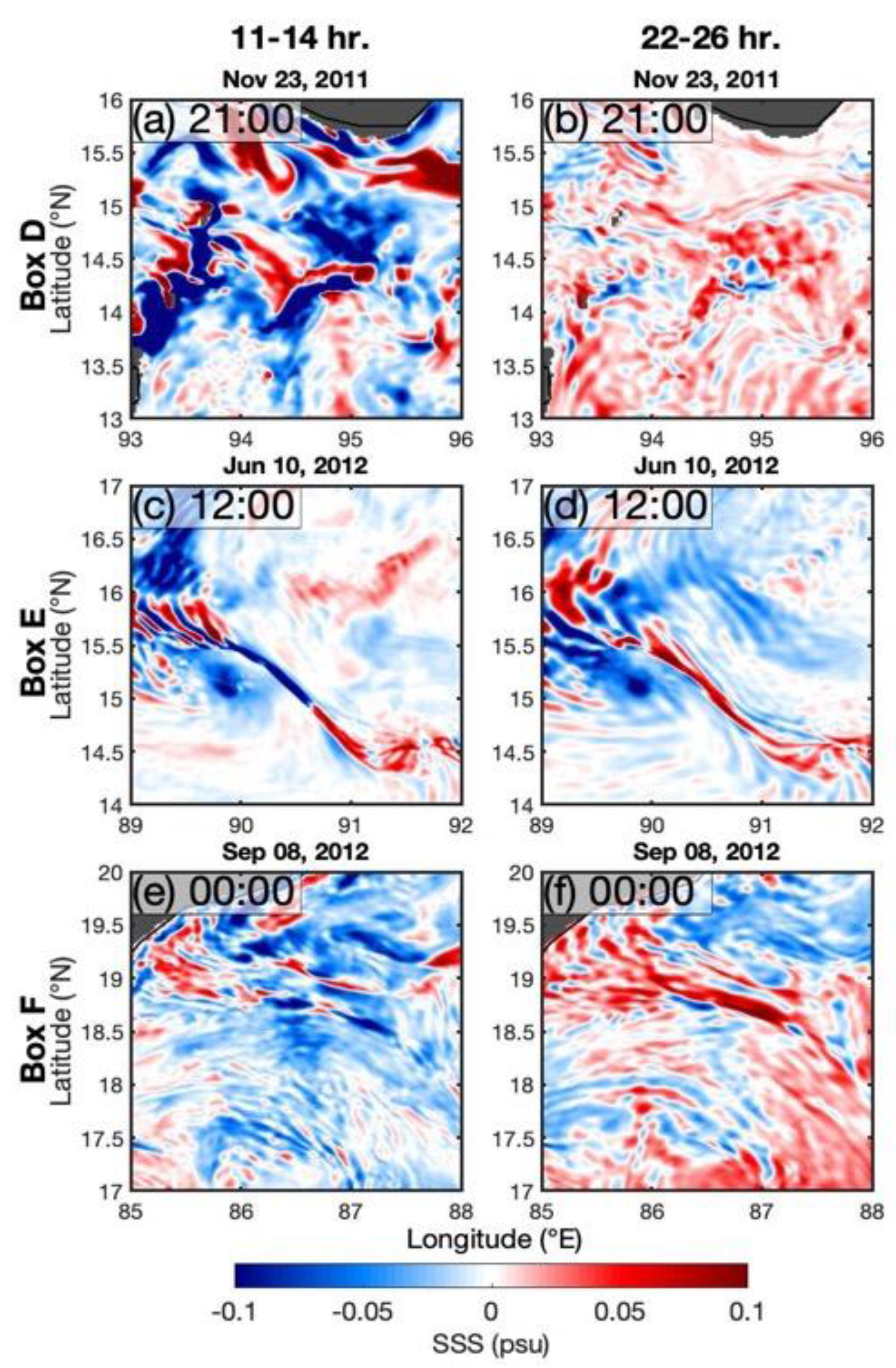
Table 1.
Estimated parameters of semi-diurnal period Internal Tide in each box A to F and their propagation direction, resultant wavenumber (k, 1/degree), wavelength (km), period (hour), and speed (m/s) as derived from 2D-FFT spectra plots for boxes A to F using the 11–14 h bandpass filtered time series data of ECCO salinity (Figure 10 and Figure 12).
| IW Category | Box | Propagation Direction | k (1/degree) | Wavelength (km) | Period (h) | Speed (m/s) |
|---|---|---|---|---|---|---|
| Semi-diurnal (11–14 h) | Box A | Northeast | 10.202 | 10.880 | 12.722 | 0.238 |
| Box B | Southwest | 6.306 | 17.602 | 12.773 | 0.383 | |
| Box C | Southwest | 3.899 | 28.468 | 13.263 | 0.596 | |
| Box D | Southwest | 8.902 | 12.468 | 12.896 | 0.269 | |
| Box E | Southwest | 3.158 | 35.144 | 12.387 | 0.788 | |
| Box F | Southwest | 8.219 | 13.506 | 12.082 | 0.311 |
Table 2.
Estimated parameters of diurnal period Internal Tide in each box A to F and their propagation direction, resultant wavenumber (k, 1/degree), wavelength (km), period (hour), and speed (m/s) as derived from 2D-FFT spectra plots for boxes A to F using the 22–26 h bandpass-filtered time series data of ECCO salinity.
| Internal Tide Category | Box | Propagation Direction | k (1/degree) | Wavelength (km) | Period (h) | Speed (m/s) |
|---|---|---|---|---|---|---|
| Diurnal (22–26 h) | Box A | Northeast | 2.418 | 45.899 | 23.572 | 0.541 |
| Box B | Southwest | 8.933 | 12.425 | 23.576 | 0.146 | |
| Box C | Southwest | 11.327 | 9.799 | 23.491 | 0.116 | |
| Box D | Southwest | 6.865 | 16.169 | 23.794 | 0.189 | |
| Box E | Southwest | 6.865 | 16.169 | 23.877 | 0.188 | |
| Box F | Southwest | 6.306 | 17.602 | 24.165 | 0.202 |
Disclaimer/Publisher’s Note: The statements, opinions and data contained in all publications are solely those of the individual author(s) and contributor(s) and not of MDPI and/or the editor(s). MDPI and/or the editor(s) disclaim responsibility for any injury to people or property resulting from any ideas, methods, instructions or products referred to in the content. |
© 2023 by the authors. Licensee MDPI, Basel, Switzerland. This article is an open access article distributed under the terms and conditions of the Creative Commons Attribution (CC BY) license (https://creativecommons.org/licenses/by/4.0/).
Share and Cite
MDPI and ACS Style
Subrahmanyam, B.; Murty, V.S.N.; Hall, S.B. Characteristics of Internal Tides from ECCO Salinity Estimates and Observations in the Bay of Bengal. Remote Sens. 2023, 15, 3474. https://doi.org/10.3390/rs15143474
AMA Style
Subrahmanyam B, Murty VSN, Hall SB. Characteristics of Internal Tides from ECCO Salinity Estimates and Observations in the Bay of Bengal. Remote Sensing. 2023; 15(14):3474. https://doi.org/10.3390/rs15143474
Chicago/Turabian StyleSubrahmanyam, Bulusu, V.S.N. Murty, and Sarah B. Hall. 2023. "Characteristics of Internal Tides from ECCO Salinity Estimates and Observations in the Bay of Bengal" Remote Sensing 15, no. 14: 3474. https://doi.org/10.3390/rs15143474
Note that from the first issue of 2016, this journal uses article numbers instead of page numbers. See further details here.