Article

A Modified Frequency Nonlinear Chirp Scaling Algorithm for High-Speed High-Squint Synthetic Aperture Radar with Curved Trajectory

1
State Key Lab of Millimeter Waves, Southeast University, Nanjing 210096, China
2
Hwa Create Technology Cop., Ltd., Beijing 100193, China
*
Author to whom correspondence should be addressed.
Remote Sens. 2024, 16(9), 1588; https://doi.org/10.3390/rs16091588
Submission received: 25 October 2023 / Revised: 1 January 2024 / Accepted: 12 January 2024 / Published: 29 April 2024

Abstract

:
The imaging of high-speed high-squint synthetic aperture radar (HSHS-SAR), which is mounted on maneuvering platforms with curved trajectory, is a challenging task due to the existence of 3-D acceleration and the azimuth spatial variability of range migration and Doppler parameters. Although existing imaging algorithms based on linear range walk correction (LRWC) and nonlinear chirp scaling (NCS) can reduce the range–azimuth coupling of the frequency spectrum (FS) and the spatial variability of the Doppler parameter to some extent, they become invalid as the squint angle, speed, and resolution increase. Additionally, most of them ignore the effect of acceleration phase calibration (APC) on NCS, which should not be neglected as resolution increases. For these issues, a modified frequency nonlinear chirp scaling (MFNCS) algorithm is proposed in this paper. The proposed MFNCS algorithm mainly includes the following aspects. First, a more accurate approximation of range model (MAARM) is established to improve the accuracy of the instantaneous slant range history. Second, a preprocessing of the proposed algorithm based on the first range compression, LRWC, and a spatial-invariant APC (SIVAPC) is implemented to eliminate most of the effects of high-squint angle and 3-D acceleration on the FS. Third, a spatial-variant APC (SVAPC) is performed to remove azimuth spatial variability introduced by 3-D acceleration, and the range focusing is accomplished by the bulk range cell migration correction (BRCMC) and extended secondary range compression (ESRC). Fourth, the azimuth-dependent characteristics evaluation based on LRWC, SIVAPC, and SVAPC is completed to derive the MFNCS algorithm with fifth-order chirp scaling function for azimuth compression. Consequently, the final image is focused on the range time and azimuth frequency domain. The experimental simulation results verify the effectiveness of the proposed algorithm. With a curved trajectory, HSHS-SAR imaging is carried out at a 50° geometric squint angle and 500 m × 500 m imaging width. The integrated sidelobe ratio and peak sidelobe ratio of the point targets at the scenario edges approach the theoretical values, and the range-azimuth resolution is 1.5 m × 3.0 m.

Graphical Abstract

1. Introduction

As an active microwave sensor, synthetic aperture radar (SAR) is capable of providing high-resolution 2-D imagery of a long-distance detection area under all weather conditions and at all times. This is due to its electromagnetic wave characteristics and motion imaging mechanism [1]. With the rapid advancement of SAR systems, they have been widely applied to high-speed maneuvering platforms, including airplanes [2,3,4,5], missiles [6,7,8,9], and unmanned aerial vehicles [10,11,12,13] for flight navigation, terminal guidance, and autonomous landing in areas of interest. Among the modes and applications mentioned above, the high-speed SAR system has several distinct features that require special consideration in SAR imaging algorithms. These features include high-squint angle, azimuth spatial variability of Doppler parameters, real-time processing, and curved trajectory [14,15].
Basically, SAR imaging algorithms can be divided into three main categories: time-domain algorithms [16,17,18,19], frequency-domain algorithms [20,21,22,23], and wavenumber-domain algorithms [24,25,26,27]. Time-domain algorithms, such as the back-projection (BP) algorithm, have essential applicability for high-squint angle and curved trajectory with high resolution [28,29]. The intensive computation burden limits the real-time application of time-domain algorithms, even though several accelerated BP algorithms are proposed. Wavenumber-domain algorithms, most of which include Stolt interpolation, can deal with cases of high-squint angle [30,31]. However, they can hardly handle the azimuth spatial variability of Doppler parameters while also dealing with the increased computational complexity of high-squint high-speed SAR (HSHS-SAR) with curved trajectory. Frequency-domain algorithms can provide a favorable balance between imaging accuracy and efficiency in this scenario.
The classical frequency-domain algorithms, which are based on the range-Doppler (RD) algorithm [32] or the chirp scaling (CS) algorithm [33,34,35], normally use range cell migration correction (RCMC) and secondary range compression (SRC) to remove range–azimuth coupling (RAC). Then, they can hardly be applied to the case of high-squint angle due to extremely severe RAC [36,37]. Therefore, multiple nonlinear CS (NCS) algorithms [38,39,40,41,42,43,44,45,46] are presented to decoupled the RAC. To remove more severe RAC of the signal, the third-order CS function was used at first [38,39,40,41]. To further increase the image precision, the CS function was then upgraded to the fourth order [42]. Afterwards, NCS processing has been used for numerous processing methods or working modes, such as fractional chirp scaling algorithm (FrCSA) [43], 2D NCS [44], Blind NCS [45], and Mosaic SAR [46]. Specifically, An et al. [47] proposed a modified azimuth NCS algorithm by using a fourth-order CS function to realize highly squint airborne SAR imaging. However, the azimuth spatial variability of Doppler parameters needs to be considered for HSHS-SAR with curved trajectory. In addition, Li et al. [48] proposed a frequency domain imaging algorithm based on tandem two-step nonlinear chirp scaling (TNCS) with small aperture. Unfortunately, most of the NCS algorithms are invalid with increased speed, squint angle, and resolution; thus, a more accurate range model and higher-order CS function should be implemented to improve the performance of the NCS algorithm.
Fundamentally, NCS algorithms, which deal with curved trajectory, utilize the linear range walk correction (LRWC) to decouple RAC. And when SAR systems move with 3-D acceleration, it is indispensable to eliminate its impact on Doppler bandwidth (DB), i.e., acceleration phase calibration (APC), which will introduce range distortion similar to those caused by the LRWC operation. Most of the NCS algorithms only consider the distortion resulting from LRWC when performing NCS processing. However, the distortion caused by the removal of 3-D acceleration cannot be ignored, especially when the resolution is increasing.
Motivated by the discussion above, a modified frequency NCS (MFNCS) algorithm with fifth-order CS function for HSHS-SAR with curved trajectory is proposed in this paper. First, a more accurate approximation of range model is established to enhance phase accuracy. Then, in order to primarily eliminate the influence of high-squint angle and 3-D acceleration, a pre-processing of the proposed algorithm is conducted via the LRWC and a spatial-invariant APC (SIVAPC). Afterward, range focusing is implemented by a spatial-variant APC (SVAPC) and bulk compensation processing, including bulk RCMC (BRCMC) and extended SRC (ESRC). Subsequently, the azimuth-dependent characteristics of NCS algorithms based on the LRWC, SIVAPC, and SVAPC are analyzed to derive the MFNCS algorithm with a fifth-order CS function for azimuth compression. Finally, the final image is focused on the range time and azimuth frequency domain. The main innovations of the proposed method are listed below.
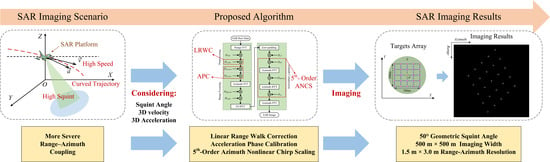
  • A more accurate approximation of the range model is proposed, along with an MFNCS algorithm that utilizes a fifth-order CS function. Although several NCS algorithms exist for HSHS-SAR with curved trajectory, most of them utilize fourth-order CS functions to mitigate the azimuth spatial variability of Doppler parameters. However, these algorithms are not suitable when the squint angle, speed, and resolution are increasing. To address this problem, a more precise range model approximation is established, and an MFNCS algorithm with a fifth-order CS function is derived to accommodate the improved accuracy of the range model.
  • The impacts of the LRWC, SIVAPC, and SVAPC are analyzed in the azimuth NCS processing. When SAR systems move with 3-D acceleration, it is necessary to eradicate its effects on the DB, i.e., the effects of the SIVAPC and SVAPC in this paper. However, most of the existing NCS algorithms only consider the range distortion introduced by the LRWC operation. Then, this will result in azimuth defocusing due to improved azimuth resolution. Hence, the effects of the SIVAPC and SVAPC are also discussed in the azimuth NCS processing to enhance the azimuth focusing capability.
The contents of this paper are organized as follows. Section 2 deeply analyzes the HSHS-SAR imaging geometry model with the proposed range approximation. Section 3 presents the preprocessing of the proposed algorithm for HSHS-SAR with curved trajectory. Section 4 depicts range focusing via the SVAPC. In Section 5, an MFNCS algorithm with a fifth-order CS function is derived in detail. Section 6 shows the results of simulation data. The analysis and discussion of the proposed algorithm is given in Section 7. Finally, the conclusion is drawn in Section 8.

2. Signal Model

2.1. Range Model

Assume that the HSHS-SAR system satisfies the start-stop approximation, and its imaging geometry is shown in Figure 1. It moves along the curved trajectory A B D during the synthetic aperture time t a with 3-D velocity v = v x , v y , v z and 3-D acceleration a = a x , a y , a z in the Cartesian coordinates O X Y Z , respectively. Here, B 0 , 0 , h is the position corresponding to the azimuth time t a = 0 , and the point C is an arbitrary position on the trajectory A B D . At azimuth time t a , the coordinates of point C can be expressed as
C v x t a + 1 2 a x t a 2 , v y t a + 1 2 a y t a 2 , v z t a + 1 2 a z t a 2 + h .
The point P x 0 , y 0 , 0 is the reference point of imaging scene S on the ground plane O X Y , whose reference slant range is R 0 with geometric squint angle θ A and residual angle of zero-Doppler squint angle ϑ . According to the geometric definition in Figure 1, the coordinates of point P can be obtained by
x 0 = R 0 sin θ A , y 0 = R 0 2 cos 2 θ A h 2 .
The point Q is an arbitrary position in the scene S. Assume that the beam centerline time is t n , then the coordinates of point Q can be derived as
Q v x t n + 1 2 a x t n 2 + x 0 , v y t n + 1 2 a y t n 2 + y 0 , v z t n + 1 2 a z t n 2 .
Thus, the instantaneous slant range history (ISRH) can be approximated by the fourth-order Taylor series (TS) as [1]
R t a , R 0 = C Q R 0 + i = 1 4 k i t a t n i ,
where k i = 1 / i ! d i R t a , R 0 / d t a i t a = t n denotes the coefficient of TS.
Herein, it is necessary to analyze the slant range error of (4) to guarantee the reliability of the following algorithm. The range error can be expressed as
Δ R = C Q R 0 + i = 1 4 k i t a t n i .
The phase error in (4) can be written as Δ ϕ = j 4 π Δ R / λ , where λ denotes the LFM signal wavelength. It is worth mentioning that the range and phase errors are accumulated with the azimuth synthetic aperture time (ASAT) and the azimuth illumination time (AIT). Essentially, AIT is the scope of t n .
Then, the range error and phase error simulations are performed, as shown in Figure 2. Table 1 lists the simulation parameters. The ASAT and AIT are set from −0.25 s to 0.25 s and −1.0 s to 1.0 s, respectively. As can be seen, the overall scenario’s phase error is fundamentally less than π / 4 , while the range error is much less than one wavelength, i.e., λ . As a result, it is feasible to utilize the 4th-order Taylor expansion approximation model.

2.2. Model Characteristics of the Range Model

In order to further analyze the spatial variability of the range model, it is required to expand k i into a polynomial with respect to t n , dividing them into k i j v (related only to velocity v ) and k i j a (affected by acceleration a ) at the same time, i.e.,
k i = j = 0 i k i j t n j , k i j = k i j v + k i j a 1 i 4 , 0 j i ,
where the detailed coefficients k i of TS are shown in Appendix A.
As can be observed in (A3) and (A4), all k i j v are not coupled with t n , implying that the spatial-variants (SVs) of k i are all generated by a , which is a prominent feature of HSHS-SAR signal with curved trajectory. Specifically, the space-invariant (SIV) of k 1 is related only to v and its SV is affected only by a , which facilitates subsequent uniform processing. The SIVs of k i (i = 2, 3, 4) consist of k i j v and k i j a , but their SVs only incorporate k i j a . This is quite different from the traditional SAR range model without acceleration. Additionally, it is important to note that k i can only be expanded into an i-th polynomial with respect to t n , which is the key factor in the approximation of the ISRH.

2.3. Accuracy Analysis of Range Model

Based on the characteristics of this range model, the ISRH can be divided succinctly into SIVs and SVs with respect to R 0 and t n . And then these two components can be further classified as range and Doppler. In general, the range SIVs and SVs are insensitive to variation in slant range, so the range-dependent spatial-variant error can be directly eliminated by range blocking [47]. However, the Doppler SVs are susceptible to changes in azimuth time. Thereby, only the spatial-variant terms in azimuth direction with R = R 0 need analysis, as shown in (6). Currently, most accurate approximations of the ISRH only retain the SIV and linear SV of k 3 and the SIV of k 4 . This approximation is not sufficiently accurate as resolution is increasing. Herein, in order to improve the imaging accuracy, a more accurate approximation of range model (MAARM), which also maintains the quadratic SV of k 3 and linear SV of k 4 , is proposed. And the detailed approximation can be formulated as
k 1 R 0 , t n = k 10 v + k 11 a t n , k 2 R 0 , t n = k 20 v + k 20 a + k 21 a t n + k 22 a t n 2 , k 3 R 0 , t n = k 30 v + k 30 a + k 31 a t n + k 32 a t n 2 , k 4 R 0 , t n = k 40 v + k 40 a + k 41 a t n .
Consequently, the residual range error (RRE) can be expressed as
Δ R r e s = C Q R 0 + i = 1 4 k i t a t n i + k 33 a t n 3 t a t n 3 + k 42 a t n 2 + k 43 a t n 3 + k 44 a t n 4 t a t n 4 .
And the residual phase error (RPE) can be expressed as Δ ϕ r e s = j 4 π Δ R r e s / λ .
A comparison between the current approximation model and MAARM is offered to demonstrate the advantages of the MAARM. The simulation parameters are identical to those found in (5). Figure 3 and Figure 4, respectively, demonstrate the range and phase errors of these two approximations. It is evident that the RRE of the MAARM is significantly lower than that of the current approximation model, as shown in Figure 3a,b. Furthermore, Figure 4 demonstrates that the RPE of the MAARM is significantly less than the amount while the RPE of the current approximate model is mostly greater than π / 4 . Remarkably, both the RPE and RRE of the MAARM are nearly identical to those of the proposed ISRH model approximated by the 4th-order Taylor expansion. Then, in theory, the HSHS-SAR with curved trajectory can be handled more effectively by the MAARM.

2.4. Echo Signal Model

Suppose that the transmit signal is the linear frequency modulation (LFM) signal. Therefore, the echo signal on baseband from the target Q in the range frequency domain can be given as [1,49,50].
S s f r , t a ; R t a , R 0 = A w r f r a a t a exp j π f r 2 γ · exp j 4 π f c + f r c R t a , R 0 ,
where w r · denotes the range envelope in the frequency domain, a a · denotes the azimuth envelope in the azimuth time domain, A is the signal amplitude, γ is the range chirp rate, c is the speed of the light, f c and f r are the carrier frequency and range frequency, respectively. Herein, w r · , a a · , and A do not affect the derivation of the proposed algorithm, and thus they can be omitted in the subsequent derivations.

3. Preprocessing Based on FRC and LRWC

3.1. FRC and LRWC

Due to the characteristics of the LFM signal, the first exponential term can be removed by range pulse compression [1], and then the filter of the first range compression (FRC) can be expressed as
H F R C f r = exp j π f r 2 γ .
The high-squint angle mode (HSAM) introduces a skew frequency spectrum (FS), which results in severe RAC and will make it challenging to perform unified processing of the echo signals. According to (4), (7) and (9), the main coupled term caused by the HSAM is the constant term of k 1 , specifically the linear range walk term k 10 v . Thus, the skew frequency spectrum can be decoupled largely by the LRWC [27], and its filter can be given as
H L R W C f r , t a ; R 0 = exp j 4 π f c + f r c k 1 v t a .

3.2. Impacts of Acceleration and SIVAPC

Compared to the classical range model without acceleration, 3-D acceleration leads to an expansion or contraction of the azimuth FS. According to the formula for Doppler parameters [48], the DB with 3-D acceleration can be expressed as
B a 3 a = T a 2 π d 2 φ a d t a 2 = 4 T a λ k 2 + 3 k 3 t a t n + 6 k 4 t a t n 2 ,
where T a and φ a denote the synthetic aperture time and azimuth time phase, respectively.
In order to delineate the effect of 3-D acceleration on the DB, a ductility factor (DF) with 3-D acceleration is defined as the ratio between the B a 3 a and B a (DB of the no-acceleration model), which can be described as
F d = B a 3 a B a = k 2 + 3 k 3 t a t n + 6 k 4 t a t n 2 k 20 v + 3 k 30 v t a t n + 6 k 40 v t a t n 2 .
Also, a simulation of the DF based on the parameters in Table 1 is performed. The ASAT is set from −0.25 s to 0.25 s, the AIT is set from −1.0 s to 1.0 s, and two additional sets of acceleration parameters are set as (18, 0.01, −25) m/s2 and (18, 0.01, 25) m/s2. The visualization of the DF is shown in Figure 5. It is evident that the DF with 3-D acceleration exhibits spatial variability. Moreover, different acceleration parameters have distinct effects on the DF, which could potentially lead to excessive or insufficient DF values. These two scenarios indicate that the DB is either expanded or compressed, resulting in FS aliasing and distortion.
According to (13), the main impact factors of F d are its SIVs. Then, in order to clearly illustrate the relationship between 3-D acceleration and DB, t n is set to 0 and both a x and a z are set from −1000 m/s2 to +1000 m/s2 in the two controlled experiments. Also, the DF, which is based on the parameters in Table 1, is recalculated and the simulation results are displayed in Figure 6. Evidently, the DF exhibits approximate linear correlations with a x and a z . The rate of change is substantial, and in certain instances the DF tends to approach 0. Subsequently, the PRF cannot satisfy Nyquist’s Sampling Law, and the FS is severely compressed and distorted. Therefore, it is essential to eliminate the effects of acceleration, and a spatial-invariant APC (SIVAPC) is proposed to restore the DB for subsequent 2-D frequency domain processing. In this context, its filter can be expressed as
H S I V A P C f r , t a ; R 0 = exp j 4 π f c + f r c i = 2 4 k i 0 a t a i .
After the FRC, LRWC, and SIVAPC, the signal in the range frequency domain can be formulated as
S s 1 f r , t a ; R 0 , t n = exp j 4 π f c + f r c i = 0 4 s i t a t n i ,
where
s 0 = R 0 k 10 v t n k 20 a t n 2 k 30 a t n 3 k 40 a t n 4 , s 1 = 3 k 30 a t n 2 4 k 40 a t n 3 , s 2 = k 20 v + k 21 a 3 k 30 a t n + k 22 a 6 k 40 a t n 2 t a t n 2 , s 3 = k 30 v + k 31 a 4 k 40 a t n + k 32 a t n 2 t a t n 3 , s 4 = k 40 v + k 41 a t n t a t n 4 .
As can be seen, the DF of (15), which is illustrated in Figure 7, approximates to 1, signifying that the DB with 3-D acceleration approaches to the DB without 3-D acceleration. Therefore, this preprocessing is suitable for most of the existing HSHS-SAR imaging algorithms.
Although the SIVs, which are caused by 3-D acceleration, are removed by the aforementioned preprocessing, the SVs should also be further eliminated for range focusing and azimuth compression. Herein, the specific derivation of the range focusing and azimuth compression is described in the next two sections, i.e., Section 4 and Section 5.

4. Range Focusing via SVAPC

As mentioned above, the range SVs can be omitted at short range widths by blocking, but the Doppler SVs with 3-D acceleration will introduce additional range cell migration (RCM), which should be tackled first by a spatial-variant APC (SVAPC).

4.1. SVAPC

According to (15), the highest term of SVs is the linear term of t a t n 4 , which can be compensated by a fifth-order phase filter as follows
H S V A P C f r , t a ; R 0 = exp j 4 π f c + f r c i = 3 5 L i t a i ,
where L i (i = 3, 4, 5) are the coefficients to be determined. In order to remove the main components of SVs, we multiply (16) with (15) and set the coefficients of t a t a t n 2 , t a t a t n 3 , and t a t a t n 4 to zero. Then, L i can be obtained as
L 3 = k 30 a 1 3 k 21 a , L 4 = k 40 a 1 4 k 31 a , L 5 = 1 5 k 41 a .
Additionally, substitute L i (i = 3, 4, 5) into (16) and multiply it by (15), whereby the signal after the SVAPC can be obtained as
S s 2 f r , t a ; R 0 , t n = exp j 4 π f c + f r c i = 0 5 K i t a t n i ,
where
K 0 = R 0 k 10 v t n k 20 a t n 2 1 3 k 21 a t n 3 1 4 k 31 a t n 4 1 5 k 41 a t n 5 , K 1 = k 21 a t n 2 k 31 a t n 3 k 41 a t n 4 , K 2 = k 20 v + k 22 a 3 2 k 31 a t n 2 2 k 41 a t n 3 , K 3 = k 30 v + k 30 a 1 3 k 21 a + k 32 a 2 k 41 a t n 2 , K 4 = k 40 v + k 40 a 1 4 k 31 a , K 5 = 1 5 k 41 a .

4.2. BRCMC and ESRC

Next, the BRCMC and ESRC need to be performed in the 2-D frequency domain. In this context, the 2-D FS of the signal can be obtained by the fast Fourier transform (FFT), which mainly utilizes the principle of stationary phase (POSP) and the method of series reversion (MSR) [51], and then it is expanded by a third-order TS, yielding [49,50]
S S 2 f r , f a ; R 0 , t n = exp j 4 K 0 c f r exp j π φ f r , f a ,
where
φ f r , f a = φ a z f a ; R 0 , t n + φ r c m f a ; R 0 , t n f r + φ q r f a ; R 0 , t n f r 2 + φ c r f a ; R 0 , t n f r 3 .
In (19), the first exponential term consists of range information of the target. And φ a z , φ r c m , φ q r , and φ c r denote the azimuth phase, RCM term, quadratic range frequency modulation (FM) term, and cubic range FM term, respectively. The detailed expression of (19) is shown in Appendix B.
As can be seen in (A5)–(A8), they are quite complicated due to the presence of K 1 which is the spatial-variant residual Doppler center introduced by 3-D acceleration. Fortunately, its spatial-variant effect on the range envelope is so weak that the φ r c m , φ q r , and φ c r can be simplified by setting t n to 0 [48]. The specific analysis will be elaborated in Section 4.3. Thus, the filter of the BRCMC and ESRC can be given as
H B R C M C f r , f a ; R 0 = exp j π φ r c m f a ; R 0 , 0 f r = exp j π + λ 4 K 2 f c f a 2 + K 3 λ 2 8 K 2 3 f c f a 3 + 3 λ 3 α 256 K 2 5 f c f a 4 + λ 4 β 256 K 2 7 f c f a 5 f r , H E S R C f r , f a ; R 0 = exp j π φ q r f a ; R 0 , 0 f r 2 + φ c r f a ; R 0 , 0 f r 3 = exp j π λ 4 K 2 f c 2 f a 2 + 3 K 3 λ 2 16 K 2 3 f c 2 f a 3 + 3 λ 3 α 128 K 2 5 f c 2 f a 4 + 5 λ 4 β 512 K 2 7 f c 2 f a 5 f r 2 + λ 4 K 2 f c 3 f a 2 + K 3 λ 2 4 K 2 3 f c 3 f a 3 + 5 λ 3 α 128 K 2 5 f c 3 f a 4 + 5 λ 4 β 256 K 2 7 f c 3 f a 5 f r 3 .
In contrast to the traditional SRC, it should be noted that the filter of the ESRC compensates for both φ q r and φ c r , improving the accuracy of the range focusing. The range signal is focused by transforming the 2-D FS into the 2-D time domain as follows
s s 3 t r , t a ; R 0 , t n = sinc B r t r 2 K 0 c exp j 4 π λ i = 0 5 K i t a t n i ,
where B r and t r denote range bandwidth and range time, respectively.

4.3. Accuracy Analysis of BRCMC and ESRC

As mentioned above, the operations of the BRCMC and ESRC involve a certain level of approximation, where the residual Doppler center, i.e., K 1 = 0, is ignored. Therefore, an analysis of its accuracy is necessary. According to (19) and (20), the RCM error of the BRCMC and ESRC operation can be formulated as
Δ B R C M C = λ 4 φ r c m f a ; R 0 , t n φ r c m f a ; R 0 , 0 f r , Δ E S R C = λ 4 φ q r f a ; R 0 , t n φ q r f a ; R 0 , 0 f r 2 + φ c r f a ; R 0 , t n φ c r f a ; R 0 , 0 f r 3 .
Then, the total RCM error can be easily expressed as
Δ R C M = Δ B R C M C + Δ E S R C .
To provide a more intuitive visualization of the accuracy of the BRCMC and ERC, we conducted a simulation of the Δ R C M using the parameters listed in Table 1, as shown in Figure 8. The AIT is set to 0.2 s, 0.5 s, and 1.0 s, respectively, to compare their spatial-variant properties. Inspecting Figure 8a–c, it can be observed that the Δ R C M increases with increasing t n and is far less than 1 m. This demonstrates that the accuracy of the BRCMC and ERC is applicable for HSHS-SAR with the curved trajectory.

5. Azimuth Compression Based on the MFNCS Algorithm

5.1. Zero-Padding and Cascade Processing

Basically, the MFNCS operation will cause the extension of the signal time-width by adding a perturbation factor (PF). Hence, in order to avoid imaging aliasing, the zero-padding operation should be adopted in the azimuth time domain before azimuth processing, and the azimuth zero-padding analysis can be seen in [27]. Herein, the zero-padding factor can be set to 2 or 4 for high-squint angle.
Due to the SVAPC operation with a fifth-order phase filter, the spatial-variant continuity of the azimuth time phase φ a z is broken, impairing the applicability of the FNCS function. Thus, it is necessary to implement a cascade factor (CF) to eliminate the effect of the SVAPC on φ a z . Then, according to (16), the CF term can be obtained by
H C F t a ; R 0 = exp j 4 π λ i = 3 5 L i t a i .
Then, the signal after the cascade processing can be expressed as
s s 4 t r , t a ; R 0 , t n = sinc B r t r 2 K 0 c exp j 4 π λ i = 0 4 s i t a t n i .

5.2. Azimuth-Dependent Characteristics Evaluation

As can be seen in (25), targets within the same range R 0 but at different AIT t n are focused onto different range cells K 0 using the LRWC, SIVAPC, and SVAPC operation. Thus, in order to fulfil the azimuth unified processing, it is imperative to substitute K 0 for R 0 as the new reference range cell. Importantly, the impact of the SIVAPC and SVAPC should be considered together because of the complicated nonlinear relationship between K 0 and t n . Thus, an extended approximation is established as
K 0 R 0 k 10 v t n k 20 a t n 2 .
Herein, the cubic and higher order terms of t n in K 0 are omitted.
It is important to note that most classical algorithms only consider the effect of the LRWC by keeping the constant and linear term of K 0 . For the purpose of analyzing the accuracy of these two approximations more clearly, their errors of K 0 should be compared. According to (18) and (26), the error of the proposed approximation can be expressed as
Δ K = 1 3 k 21 a t n 3 + 1 4 k 31 a t n 4 + 1 5 k 41 a t n 5 .
Then, the simulation of Δ K is carried out using the parameters listed in Table 1, where the range width is set from −1.5 km to 1.5 km and AIT is set from −1.0 s to 1.0 s. The Δ K values for the proposed and classical approximation are shown in Figure 9a,b, respectively. It is evident that the accuracy of the proposed approximation is high enough to be applicable. However, the Δ K of the classical approximation is even larger than a few range cells when AIT is large. Therefore, the proposed approximation of K 0 has better adaptability for HSHS-SAR with curved trajectory. Additionally, the trend of Δ K in Figure 9 indicates that the Δ K is not sensitive to range-dependent variability but is strongly influenced by azimuth-dependent variability.
Suppose that the conditions v y v x , v z , a y a x , a z are satisfied, whereby then the spatial variability of σ 1 can be neglected. The quadratic Equation (26) can then be solved, and the solution is
R 0 = K 0 2 δ 3 t n 2 δ 4 t n 2 4 + 2 K 0 δ 4 t n 2 2 8 K 0 δ 3 + 2 δ 1 t n + 4 δ 3 2 2 δ 2 t n 2 + 4 δ 3 δ 4 t n 3 4 ,
where δ 1 = v y σ 1 v z h , δ 2 = a y σ 1 a z h , δ 3 = v x sin θ A , δ 4 = a x sin θ A .
Then, R 0 in (25) is substituted by K 0 utilizing (28), and the azimuth signal will be rewritten as
s s 4 t r , t a ; K 0 , t n = sinc B r t r 2 K 0 c exp j 4 π λ i = 0 4 d i t a t n i ,
where d i is related to K 0 instead of R 0 .

5.3. Derivation of MFNCS Algorithm

Before performing the MFNCS operation, the PF of the high-order phase (HOP) should be embedded in (29) to align the azimuth phase for subsequent uniform processing. Meanwhile, the highest-order term in (29) is the linear term of its fourth-order phase [47]. Then, in order to adjust the overall phase, the PF of the HOP should be a fifth-order polynomial. Thus, the filter of the PF can be expressed as
H P F t a ; K 0 = exp j 4 π λ i = 3 i = 5 C i K 0 t a i ,
where C i ( K 0 ) corresponds to each range cell and are required to be determined. Then, we multiply (30) and (29), and then transform the signal into the azimuth frequency domain utilizing the POSP and MSR, yielding
s S 5 t r , f a ; K 0 , t n = sinc B r t r 2 K 0 c exp ( j 4 π J 0 λ ) exp j π φ a z 1 f a ; K 0 , t n ,
φ a z 1 f a ; K 0 , t n = 2 f a t n + λ 4 J 2 f a + 2 λ J 1 2 + λ 2 J 3 16 J 2 3 f a + 2 λ J 1 3 + λ 3 α ^ 256 J 2 5 f a + 2 λ J 1 4 + λ 4 β ^ 1024 J 2 7 f a + 2 λ J 1 5 ,
where
K 0 = R 0 k 10 v t n k 20 a t n 2 , J 0 = R 0 k 10 v t n k 20 a t n 2 + C 3 k 30 a t n 3 + C 4 k 40 a t n 4 + C 5 t n 5 , J 1 = 3 C 3 3 k 30 a t n 2 + 4 C 4 4 k 40 a t n 3 + 5 C 5 t n 4 , J 2 = k 20 v + k 21 a 3 k 30 a + 3 C 3 t n + k 22 a 6 k 40 a + 6 C 4 t n 2 + 10 C 5 t n 3 , J 3 = k 30 v + C 3 + k 31 a 4 k 40 a + 4 C 4 t n + k 32 a + 10 C 5 t n 2 , J 4 = k 40 v + C 4 + k 41 a + 5 C 5 t n , J 5 = C 5 , α ^ = 9 J 3 2 4 J 2 J 4 , β ^ = 4 J 5 J 2 2 24 J 4 J 2 J 3 + 27 J 3 3 .
For the purpose of simplifying the subsequently expressions, it is needed to expand J i using the TS into a polynomial form with respect to t n . Then, J i can be given as follows
J 1 = J 12 t n 2 + J 13 t n 3 + J 14 t n 4 , J 2 = J 20 + J 21 t n + J 22 t n 2 + J 23 t n 3 , J 3 = J 30 + J 31 t n + J 32 t n 2 , J 4 = J 40 + J 41 t n ,
where J i j denotes the polynomial coefficient of J i with respect to t n . And, the detailed expressions of (33) are shown in the Appendix C.
After applying a fifth-order azimuth filter, i.e., the filter of the PF, a fifth-order CS function is introduced to eliminate the azimuth-dependence of the azimuth FM rate and higher-order Doppler phase in the azimuth frequency domain. Thus, the filter of MFNCS can be presented as
H M F N C S f a ; R 0 , K 0 = exp j π i = 2 5 S i K 0 f a i ,
where S i corresponds to K 0 and is to be determined.
Then, we multiply (34) by (31) and transform the signal back into the azimuth time domain utilizing the POSP and MSR. Also, based on the accuracy analysis of the MAARM, the azimuth phase of the signal can be expanded to the order corresponding to that of (7) by the 2-D TS with respect to t a and t n at [ t a = 0, t n = 0]. Then, the signal can be fetched by
s s 6 t r , t a ; K 0 , t n = sinc B r t r 2 K 0 c exp ( j 4 π J 0 λ ) exp j π ξ a z t a ; K 0 , t n ,
where
ξ a z t a ; K 0 , t n A t a ; K 0 + B K 0 , t n + C K 0 ; S 2 t a t n + D K 0 ; S 2 , S 3 , C 3 t a t n 2 + E K 0 ; S 2 , S 3 , C 3 t a 2 t n + F K 0 ; S 2 , S 3 , S 4 , C 3 , C 4 t a 2 t n 2 + G K 0 ; S 2 , S 3 , S 4 , C 3 , C 4 t a 3 t n + H K 0 ; S 2 , S 3 , S 4 , S 5 , C 3 , C 4 , C 5 t a 3 t n 2 + I K 0 ; S 2 , S 3 , S 4 , S 5 , C 3 , C 4 , C 5 t a 4 t n .
The completed expression of (36) can be viewed in Appendix D.
The first exponential term of (35) does not affect the derivation of the MFNCS operation and is independent of t a ; hence, it has no impact on azimuth focusing and can be omitted in the subsequent derivation. Then, the characteristics of (36) should be addressed: the first term A( t a ; K 0 ) is the azimuth unified focusing phase, which is used for subsequent azimuth compression; the second term B( t n ; K 0 ) is independent of t a , which does not influence the quality of the focusing image, so then it can be neglected in subsequent derivations; the third term C( K 0 , S 2 ) is the linear coupling term between t a and t n , which describes the azimuth position information of the target, so therefore this term should be maintained; evidently, the other terms of (36) are high-order coupling terms of t a and t n , which severely impair the quality of azimuth focusing, so hence these terms should be eliminated. Consequently, the terms of (36) should be set as
C K 0 ; S 2 = 4 J 20 λ η , D K 0 ; S 2 , S 3 , C 3 = 0 , E K 0 ; S 2 , S 3 , C 3 = 0 , F K 0 ; S 2 , S 3 , S 4 , C 3 , C 4 = 0 , G K 0 ; S 2 , S 3 , S 4 , C 3 , C 4 = 0 , H K 0 ; S 2 , S 3 , S 4 , S 5 , C 3 , C 4 , C 5 = 0 , I K 0 ; S 2 , S 3 , S 4 , S 5 , C 3 , C 4 , C 5 = 0 ,
where η denotes the NCS factor, which must be chosen to be around 0.5 for reducing the geometric distortion of the target position. By solving (37), undetermined coefficients in (30) and (34) can be ascertained as
C 3 = i = 0 4 C 3 i K 0 i 5 6 2 η 1 , C 4 = i = 0 8 C 4 i K 0 i 7 24 2 η 1 2 ε 1 , C 5 = i = 0 12 C 5 i K 0 i 9 40 2 η 1 3 ε 1 2 ,
S 2 = K 0 3 λ 2 η 1 2 ε 1 , S 3 = λ 2 i = 0 4 S 3 i K 0 i + 4 12 ε 1 3 , S 4 = λ 3 i = 0 8 S 4 i K 0 i + 5 96 2 η 1 ε 1 5 , S 5 = λ 4 i = 0 12 S 5 i K 0 i + 6 960 2 η 1 2 ε 1 7 .
And, the specific expressions of (38) and (39) are given in Appendix E.
After incorporating (38) and (39) into (35) and ignoring the exponential terms that do not affect the focusing quality, the signal can be rewritten as
s s 6 t r , t a ; K 0 , t n = sinc B r t r 2 K 0 c exp j π A K 0 , t a + C K 0 , S 2 t a t n ,
where
A t a ; K 0 = i = 2 5 P i t a i , C K 0 ; S 2 = 4 J 20 λ η .
According to (41), the filter of azimuth unified compression can be obtained by
H A C t a ; K 0 = exp j π A t a ; K 0 = exp j π i = 2 5 P i t a i .
Finally, transform the signal after azimuth compression into the azimuth frequency domain, and the ultimate focusing signal can be acquired as
s S 7 t r , f a ; R 0 , K 0 , t n = sinc B r t r 2 K 0 c sinc T a f a 2 J 20 λ α t n × exp ( j 4 π J 0 λ ) exp j π B t n ,
where the exponential terms of (43) have no implications on the focusing quality since they are irrelevant to t a . Thus, the final focusing position of the target Q on the slant plane is given as
Q ^ K 0 , 2 J 20 λ η t n .
And, the flowchart of the proposed method is shown in Figure 10.

6. Simulation Results

6.1. Simulation Scenario 1

This subsection depicts a simulation experiment to confirm the effectiveness of the proposed algorithm. The key simulation parameters are listed in Table 1. In addition, windowing is not used in the processing to suppress the sidelobe. As illustrated in Figure 11, the five point targets are distributed in cross shape in this scenario. Point targets are 250 m apart in the X and Y directions. The imaging result of the proposed algorithm is displayed in Figure 12. The range-azimuth resolution is about 1.5 m × 3.0 m.
To elucidate the processing impact of the proposed algorithm, the processing results of several key steps are displayed in Figure 13 and Figure 14. Results are provided for a variety of domains, including 2D time domain, range-frequency and azimuth-time domain, range-time and azimuth-frequency domain, and 2D frequency domain.
The processing results of key steps before azimuth processing are shown in Figure 13. As can be seen in the first two rows of Figure 13, the major influence of the highly squint angle is abolished in the following LWRC operation. The 2D spectrum shows that most effects of acceleration are removed after SVAPC. In order to further analyze the validity of RCMC and ESRC, the last three subfigures in the third column of Figure 13, i.e., the image by using LWRC, SVAPC, and ESRC operations in the range-time and azimuth-frequency domain, are partially magnified, as shown in Figure 15. The red boxes in the three images above are the magnified portions. And, the signal is obviously focused on a single range cell during ESRC processing, meaning that range cell migration has been completely corrected.
Meanwhile, Figure 14 displays the processing results of important azimuth processing stages. After MFNCS processing, the 2D time-domain signal is broadened in the azimuth dimension. Hence, prior to azimuth processing, a zero-padding step is required. After AC, the signal is finally well-focused in the azimuth-frequency and range-time domain, as shown in Figure 12.

6.2. Simulation Scenario 2

To further verify the effectiveness and superiority of the proposed algorithm, a comparison simulation experiment between the proposed method and the tandem TNCS algorithm [48] is implemented in this subsection. The conditions and parameters of this simulation experiment are the same as the experiment in Section 6.1. The 5 × 5 target array (ground range × azimuth) with a scene size of 500 m × 500 m (ground range × azimuth) is set on the ground uniformly, as shown in Figure 16. Subsequently, in order to evaluate the imaging quality of the proposed method, five targets are selected, which are distributed both in the center and on the edge of the scene, as shown in Figure 17.
Their contour plots, processed by the proposed algorithm and the tandem TNCS algorithm, are given in Figure 18. The top subfigures of Figure 18 show that all targets, except for the center point target C, which are treated by the tandem TNCS algorithm, are extremely defocused in the azimuth dimension. This azimuth defocusing can be attributed to the tandem TNCS algorithm’s failure to account for the impact of APC on K 0 . Then, while considering this impact, the proposed algorithm improves the accuracy of the ISRH and utilizes a fifth-order CS function for FNCS operation, thereby greatly enhancing the quality of azimuth imaging. Thus, it can be seen in the bottom subfigures of Figure 18 that all targets, which are processed by the proposed algorithm, are well focused in both range and azimuth dimension.
In order to further analyze the azimuth focusing quality of these two algorithms, the azimuth profiles of point targets are compared, as shown in Figure 19. The top and bottom figures of Figure 19 are azimuth profiles processed by tandem TNCS algorithm and the proposed algorithm, respectively. By conducting a comparative analysis of the results obtained from these two figures, it becomes evident that the proposed algorithm demonstrates superiority over the tandem TNCS algorithm.
Furthermore, the range resolution is approximately 1.5 m. Additionally, to further analyze the performance of the proposed algorithm, the evaluations of the azimuth performance based on the proposed algorithm and the reference algorithm are presented in Table 2 and Table 3, respectively. It is evident from Table 2 that the proposed approach performs exceptionally well in imaging. The azimuth resolution (AR) is about 3.0 m, and the peak sidelobe ratio (PSLR) and integrated sidelobe ratio (ISLR) of point targets closely match the theoretical value of the Sinc function. Regarding the reference algorithm, only the performance metrics for point target C, as indicated in Table 3, match the theoretical values. Stated otherwise, the reference algorithm achieved excellent focusing on the core point target, leaving the edged point targets totally unfocused. It can be concluded that the proposed algorithm has excellent superiority over the reference algorithm and is very suitable for the simulation scenario.

7. Discussion and Analysis

7.1. Fifth-Order CS Function Applicability Analysis

As described in Section 2.2, k i of (4) can only be expanded into an i-th polynomial with respect to t n , meaning that there exists an (i-1)-order azimuth SV phase of the i-th order azimuth phase. Then, as stated in [47], in order to fulfill the application conditions of the NCS processing, the azimuth NCS processing should make approximations, i.e., ignore the comparatively higher-order SV phase. After that, the relatively lower-order azimuth SV phases can be compensated. For example, for the 4th-order CS function, its NCS processing can compensate several parts: (i) the linear part of the 3rd-order azimuth SV phase; (ii) the linear and quadratic parts of the second-order azimuth SV phase; (iii) the linear, quadratic, and cubic parts of the first-order azimuth SV phase. And it ignores the portion of other higher-order phases. Naturally, the 5th-order NCS function can adjust to the higher resolution requirement because its higher-order azimuth SV phase can be compensated more than that of the 4th-order CS function.
On the other hand, the squint angle, synthetic aperture time, azimuth imaging breadth, and other variables affect the azimuth SV phase. In the meantime, the higher-order SV phase will unavoidably be ignored by the NCS processing. Therefore, the imaging quality of the NCS algorithm degrades with increasing squint angle and azimuth imaging width. The higher the geometric squint angle, the smaller the azimuth imaging width that may be accommodated by the proposed MFNCS method which is based on a 5th-order CS function. As stated above, the 500 m azimuth imaging width can be accommodated when the geometric squint angle is about 50°.
Subsequently, an approximation, i.e., v y v x , v z and a y a x , a z , is made in the azimuth NCS processing using the suggested MFNCS method, which is based on a 5th order CS function. This indicates that the suggested algorithm is unable to adjust to the situation in which v y / v x , v y / v z , a y / a x , and a y / a z are too large. Fortunately, the effect of this approximation can be mitigated by the velocity and acceleration vector synthesis.

7.2. Geometric Distortion Analysis

According to the derivation of the MFNCS, the target Q is focused at the location ( K 0 , 2 J 20 λ η t n ) on the slant plane, and the relationship between K 0 and R 0 is
K 0 = R 0 k 10 v t n k 20 a t n 2 1 3 k 21 a t n 3 1 4 k 31 a t n 4 1 5 k 41 a t n 5 .
Thus, there is a nonlinear distortion in the focused range position, and the magnitude of range distortion can be obtained as
D Δ R = k 10 v t n + k 20 a t n 2 + 1 3 k 21 a t n 3 + 1 4 k 31 a t n 4 + 1 5 k 41 a t n 5 .
And, the azimuth position also has a retractable distortion due to the NCS factor and J 20 , and the flexible factor of azimuth distortion can be given as
D Δ t n = 2 J 20 λ η .
By observing J 20 , the azimuth distortion is associated with K 0 , indicating that the geometric distortion is coupled in two dimensions. Therefore, based on (46) and (47), the geometric correction should be implemented using 2-D Sinc interpolation, taking into account the 2-D distortion simultaneously [52].

7.3. Computational Complexity Analysis

As mentioned above, the proposed method mainly includes three procedures: (1) preprocessing of the MFNCS algorithm; (2) range focusing via the SVAPC operation; (3) azimuth compression based on the MFNCS algorithm. Then, in order to further analyze the efficiency of the proposed algorithm, a detailed discussion of computational complexity is presented here.
Assume that the SAR echo data is of N r × N a pixels, where N r and N a denote the sample points of the range and azimuth dimension, respectively. The zero-padding factor is supposed to be n in the azimuth dimension, and thus the signal data after the zero-padding operation is of N r × n N a pixels. Characteristically, all operations of the proposed algorithm contain only FFTs and complex multiplication, as shown in Figure 10. Moreover, the imaging algorithm before the zero-padding operation includes six complex multiplications, two range FFTs, and two azimuth FFTs, and it consists of four complex multiplications and three azimuth FFTs after the zero-padding operation.
According to the computer operating rules, for a data of N 1 × N 2 pixels, the computation complexity of each complex multiplication is O 6 N 1 N 2 , and the computation complexity of each FFT can be given as O 5 N 1 N 2 log 2 N 1 / 2 . Consequently, the computation complexity of the entire procedure can be calculated as
C M F N C S = O 12 3 + 2 n N r N a + 5 N r N a log 2 n 3 n N r 2 N a 3 n + 2 .
The zero-padding factor is usually set to 2 or 4 [27], which already satisfies most of the high-squint application scenarios.
The processing times of the reference method, the proposed algorithm, and the back-projection algorithm are 13.63 s, 32.96 s, and 460.07 s, respectively, when the echo data size is N r × N a = 4096 × 3584 and the zero-padding factor is 2. We implement the algorithms on a laptop with an i7-10750H and 128 GB memory. It is evident that the frequency-domain algorithm has a better efficiency than the time-domain method does. The proposed algorithm employs higher-order CS functions for NCS processing, meaning that higher-order filters need to be generated for azimuth processing, and this operation brings higher computational complexity. Fortunately, the complexity is still within an acceptable scope, and the computational efficiency can be further improved by code optimization or filter pre-generation.

8. Conclusions

In this paper, a MFNCS algorithm with a fifth-order CS function was proposed for HSHS-SAR with curved trajectory. First, a MAARM has been established to enhance the accuracy of the ISRH, and the 3-D acceleration was regarded as a parameter in the theoretical signal model. Then, a preprocessing of the proposed algorithm was depicted, which combines the FRC, LRWC, and SIVAPC to largely eliminate the effects of the LFM signal, high-squint angle, and 3-D acceleration on 2-D FS, respectively. Afterwards, range focusing has been accomplished by the SVAPC, BRCMC, and ESRC. Subsequently, the azimuth-dependent characteristics evaluation, which is influenced by the SIVAPC and SVAPC, was conducted to derive an MFNCS algorithm with a fifth-order CS function for azimuth compression. Consequently, the final image has been focused on the range time and azimuth frequency domain. Under a 50 geometric squint angle and 500 m × 500 m imaging width, the HSHS-SAR imagery with the range-azimuth resolution of 1.5 m × 3.0 m has been obtained by simulation experiment. Furthermore, by comparing the proposed algorithm with the reference algorithm, the superiority of the proposed algorithm in the simulated scenario has been demonstrated.

Author Contributions

Conceptualization, K.D. and Y.H.; Methodology, K.D.; Software, K.D.; Validation, K.D.; Formal analysis, Z.C. and D.F.; Investigation, K.D. and X.T.; Resources, Y.H., Z.C., D.F. and W.L.; Data curation, K.D.; Writing—original draft, K.D.; Writing—review and editing, K.D. and Y.H.; Visualization, K.D.; Supervision, Y.H. and W.H.; Project administration, Y.H.; Funding acquisition, Y.H. All authors have read and agreed to the published version of the manuscript.

Funding

This work was supported in part by the National Natural Science Foundation of China under Grant 62271142 and in part by the Shanghai Aerospace Science and Technology Innovation Fund under Grant SAST2021-043.

Data Availability Statement

Data are contained within the article.

Acknowledgments

The authors appreciate the anonymous referees for good suggestions in improving the paper quality.

Conflicts of Interest

Author Dongning Fu was employed by the company Hwa Create Technology Cop., Ltd. The remaining authors declare that the research was conducted in the absence of any commercial or financial relationships that could be construed as a potential conflict of interest.

Appendix A

According to the Taylor expansion formula, and in order to simplify the expression, set
σ 1 = R 0 2 cos 2 θ A h 2 , σ 2 = R 0 sin θ A , σ 3 = a x v x + a y v y + a z v z , σ 4 = a x 2 + a y 2 + a z 2 , σ 5 = v x 2 + v y 2 + v z 2 , σ 6 = v z h + v y σ 1 + v x σ 2 , σ 7 = a z h + a y σ 1 + a x σ 2 .
Then, the detailed coefficients k i , which is obtained by the TS, can be derived as
k 1 R 0 ; t n = σ 6 R 0 σ 7 R 0 t n , k 2 R 0 ; t n = σ 6 2 2 R 0 3 + σ 5 2 R 0 σ 7 2 R 0 + σ 3 R 0 σ 7 σ 6 R 0 3 t n + σ 4 2 R 0 σ 7 2 2 R 0 3 t n 2 , k 3 R 0 ; t n = σ 6 σ 5 2 R 0 3 σ 6 3 2 R 0 5 + σ 3 2 R 0 σ 6 σ 7 2 R 0 3 + σ 4 2 R 0 3 σ 7 σ 6 2 2 R 0 5 + σ 7 σ 5 σ 7 2 + 2 σ 3 σ 6 2 R 0 3 t n + σ 6 σ 4 + 2 σ 3 σ 7 2 R 0 3 3 σ 7 2 σ 6 2 R 0 5 t n 2 + σ 7 σ 4 2 R 0 3 σ 7 3 2 R 0 5 t n 3 , k 4 R 0 ; t n = σ 5 2 8 R 0 3 + 3 σ 6 2 σ 5 4 R 0 5 5 σ 6 4 8 R 0 7 + σ 4 8 R 0 + σ 3 σ 6 2 R 0 3 σ 7 2 2 σ 5 σ 7 8 R 0 3 3 σ 6 2 σ 7 4 R 0 5 + 3 σ 3 σ 6 2 σ 7 2 σ 6 + σ 7 σ 6 σ 5 2 R 0 5 5 σ 7 σ 6 3 2 R 0 7 + σ 6 σ 4 + 2 σ 3 σ 7 σ 3 σ 5 2 R 0 3 t n + 3 σ 7 σ 4 2 σ 3 2 σ 4 σ 5 4 R 0 3 15 σ 7 2 σ 6 2 4 R 0 7 + 3 σ 6 2 σ 4 σ 7 3 + σ 7 2 σ 5 + 4 σ 3 σ 7 σ 6 4 R 0 5 t n 2 + 3 σ 3 σ 7 2 + σ 7 σ 6 σ 4 2 R 0 5 σ 3 σ 4 2 R 0 3 5 σ 7 3 σ 6 2 R 0 7 t n 3 + 3 σ 7 2 σ 4 4 R 0 5 5 σ 7 4 8 R 0 7 σ 4 2 8 R 0 3 t n 4 .
Observing (A2), it is seen that k i j v contains only σ 5 and σ 6 , but k i j a comprises all the variables of (A1), thus (A2) can be decomposed as
k 1 R 0 ; t n = k 10 v + k 11 a t n , k 2 R 0 ; t n = k 20 v + k 20 a + k 21 a t n + k 22 a t n 2 , k 3 R 0 ; t n = k 30 v + k 30 a + k 31 a t n + k 32 a t n 2 + k 33 a t n 3 , k 4 R 0 ; t n = k 40 v + k 40 a + k 41 a t n + k 42 a t n 2 + k 43 a t n 3 + k 44 a t n 4 ,
where
k 10 v = σ 6 R 0 , k 11 a = σ 7 R 0 ; k 20 v = σ 5 2 R 0 σ 6 2 2 R 0 3 , k 20 a = σ 7 2 R 0 , k 21 a = σ 3 R 0 σ 7 σ 6 R 0 3 , k 22 a = σ 4 2 R 0 σ 7 2 2 R 0 3 ; k 30 v = σ 6 σ 5 2 R 0 3 σ 6 3 2 R 0 5 , k 30 a = σ 3 2 R 0 σ 6 σ 7 2 R 0 3 , k 31 a = σ 4 2 R 0 σ 7 σ 7 σ 5 2 R 0 3 + σ 3 σ 6 R 0 3 3 σ 7 σ 6 2 2 R 0 5 , k 32 a = σ 6 σ 4 2 R 0 3 + σ 3 σ 7 R 0 3 3 σ 7 2 σ 6 2 R 0 5 , k 33 a = σ 7 σ 4 2 R 0 3 σ 7 3 2 R 0 5 ; k 40 v = σ 5 2 8 R 0 3 + 3 σ 6 2 σ 5 4 R 0 5 5 σ 6 4 8 R 0 7 , k 40 a = σ 4 8 R 0 + σ 3 σ 6 2 R 0 3 σ 7 2 2 σ 5 σ 7 8 R 0 3 3 σ 6 2 σ 7 4 R 0 5 , k 41 a = σ 6 σ 4 + 2 σ 3 σ 7 σ 3 σ 5 2 R 0 3 + 3 σ 3 σ 6 2 σ 7 2 σ 6 + σ 7 σ 6 σ 5 2 R 0 5 5 σ 7 σ 6 3 2 R 0 7 , k 42 a = 3 σ 7 σ 4 2 σ 3 2 σ 4 σ 5 4 R 0 3 15 σ 7 2 σ 6 2 4 R 0 7 + 3 σ 6 2 σ 4 σ 7 3 + σ 7 2 σ 5 + 4 σ 3 σ 7 σ 6 4 R 0 5 , k 43 a = 3 σ 3 σ 7 2 + σ 7 σ 6 σ 4 2 R 0 5 σ 3 σ 4 2 R 0 3 5 σ 7 3 σ 6 2 R 0 7 , k 44 a = σ 4 2 8 R 0 3 + 3 σ 7 2 σ 4 4 R 0 5 5 σ 7 4 8 R 0 7 .

Appendix B

According to (18), the FFT of it can be obtained by the POSP and MSR, and the detailed expression of (19) is shown as follows:
φ a z f a ; R 0 , t n = 4 K 0 λ 2 f a t n + λ 4 K 2 Y 2 + λ 2 K 3 16 K 2 3 Y 3 + λ 3 α 256 K 2 5 Y 4 + λ 4 β 1024 K 2 7 Y 5 ,
φ r c m f a ; R 0 , t n = K 1 f c K 2 Y λ 2 K 2 2 3 K 1 K 3 8 K 2 3 f c Y 2 λ 2 4 K 2 2 K 3 K 1 α 32 K 2 5 f c Y 3 + λ 3 5 K 1 β 6 K 2 2 α 512 K 2 7 f c Y 4 λ 4 K 1 84 K 2 K 3 3 K 3 K 4 2 K 2 K 5 3 β 6 α 2 + 8 K 2 2 β 2048 K 2 9 f c Y 5 ,
φ q r f a ; R 0 , t n = K 1 2 K 2 λ f c 2 π K 1 4 K 2 2 3 K 1 K 3 4 K 2 3 f c 2 Y + λ 3 K 1 2 α + 8 K 2 2 K 2 2 3 K 1 K 3 32 K 2 5 f c 2 Y 2 + λ 2 5 K 1 2 β 12 K 1 K 2 2 α + 24 K 2 4 K 3 128 K 2 7 f c 2 Y 3 λ 3 15 K 1 2 K 3 28 K 2 3 K 3 K 4 2 K 2 K 5 β + 240 K 1 K 2 2 K 3 α 4 K 2 K 4 + 320 K 1 K 2 4 K 5 48 K 2 4 α 30 K 1 2 α 2 2048 K 2 9 f c 2 Y 4 + λ 4 K 1 2 105 α β 756 K 2 K 3 2 3 K 3 K 4 5 K 2 K 5 + K 1 2 α 336 K 2 K 5 K 2 3 K 4 K 3 84 β + 6 K 1 α 2 21 K 3 K 1 20 K 2 2 60 K 1 K 2 2 K 3 28 2 K 5 K 2 2 3 K 4 K 2 K 3 + β + 80 K 2 4 β 8192 K 2 11 f c 2 Y 5 ,
φ c r f a ; R 0 , t n = K 1 2 2 K 2 2 K 1 K 3 2 K 2 3 λ f c 3 + K 1 K 1 2 α + 4 K 2 2 2 K 2 2 3 K 1 K 3 8 K 2 5 f c 3 Y + λ 5 K 1 3 β 18 K 1 2 K 2 2 α + 72 K 1 K 2 4 K 3 16 K 2 6 64 K 2 7 f c 3 Y 2 λ 2 K 1 3 K 3 140 K 2 K 4 K 3 2 K 5 K 2 5 β 10 α 2 + 40 K 1 2 K 2 2 β 48 K 1 K 2 4 α + 64 K 2 6 K 3 256 K 2 9 f c 3 Y 3 + 5 λ 3 K 1 3 7 α 16 K 2 K 2 K 5 3 K 3 K 4 + β + 252 K 2 K 3 2 5 K 2 K 5 3 K 3 K 4 + 42 K 3 α 2 + K 1 2 840 K 2 3 K 3 3 K 3 K 4 2 K 2 K 5 60 K 2 2 α 2 30 β + 80 K 1 K 2 4 β 32 K 2 6 α 4096 K 2 11 f c 3 Y 4 λ 4 K 1 3 + 756 K 2 K 3 3 3 K 3 K 4 20 K 2 K 5 + α 672 K 2 K 3 9 K 3 K 4 10 K 2 K 5 840 β K 3 + 105 β 2 + α 2 448 K 2 K 4 56 α + 1120 K 2 3 K 3 K 4 K 2 K 5 β + K 1 2 1512 K 2 2 K 3 α 2 + 9072 K 2 3 K 3 2 5 K 2 K 5 3 K 3 K 4 + 4032 K 2 3 K 2 K 5 3 K 3 K 4 + 252 K 2 2 β α + K 1 10080 K 2 5 K 3 2 K 2 K 5 3 K 3 K 4 720 K 2 4 α 2 360 K 2 4 K 3 β + 320 K 2 6 β 16384 K 2 13 f c 3 Y 5 ,
where
Y = f a + 2 λ K 1 , α = 9 K 3 2 4 K 2 K 4 , β = 4 K 5 K 2 2 24 K 4 K 2 K 3 + 27 K 3 3 .

Appendix C

According to (28) and (32), J i j can be obtained by using TS as
J 12 = 3 C 3 + 3 δ 3 δ 4 σ 3 2 K 0 + 3 δ 1 δ 4 + δ 2 δ 3 2 K 0 2 + 3 δ 1 δ 2 2 K 0 3 , J 13 = 4 C 4 + δ 4 2 σ 4 2 K 0 + 2 δ 2 δ 4 2 δ 4 σ 5 7 δ 3 σ 3 + 9 δ 3 2 δ 4 2 K 0 2 + 15 δ 1 2 δ 2 2 K 0 5 + δ 2 2 + 12 δ 2 δ 3 2 2 σ 5 δ 2 + 21 δ 1 δ 3 δ 4 7 δ 1 σ 3 2 K 0 3 + 12 δ 1 2 δ 4 + 27 δ 1 δ 2 δ 3 2 K 0 4 , J 14 = 5 C 5 + 5 δ 3 δ 4 2 3 σ 3 δ 4 2 σ 4 δ 3 4 K 0 2 + 3 13 δ 1 3 δ 4 + 46 δ 1 2 δ 2 δ 3 2 K 0 6 + 8 δ 1 δ 4 2 3 δ 2 σ 3 2 δ 1 σ 4 + 30 δ 3 3 δ 4 22 σ 3 δ 3 2 δ 4 + 17 δ 2 δ 3 δ 4 8 σ 5 δ 3 δ 4 4 K 0 3 + 12 δ 2 2 δ 3 + 54 δ 2 δ 3 3 12 σ 5 δ 2 δ 3 + 23 δ 1 δ 2 δ 4 + 132 δ 1 δ 3 2 δ 4 58 δ 1 δ 3 σ 3 8 δ 1 δ 4 σ 5 4 K 0 4 + 3 60 δ 1 2 δ 3 δ 4 12 σ 3 δ 1 2 + 5 δ 1 δ 2 2 + 72 δ 1 δ 2 δ 3 2 4 σ 5 δ 1 δ 2 4 K 0 5 + 57 δ 1 3 δ 2 2 K 0 7 ;
J 20 = σ 5 2 K 0 δ 1 + K 0 δ 3 2 2 K 0 3 , J 21 = 3 C 3 + δ 3 δ 4 σ 3 2 K 0 + δ 1 δ 4 δ 3 3 + δ 2 δ 3 + σ 5 δ 3 2 K 0 2 5 δ 1 δ 3 2 δ 1 δ 2 δ 1 σ 5 2 K 0 3 7 δ 1 2 δ 3 2 K 0 4 3 δ 1 3 2 K 0 5 , J 22 = 6 C 4 + σ 4 δ 4 2 4 K 0 + 5 δ 4 σ 5 2 δ 2 δ 4 + 14 σ 3 δ 3 19 δ 3 2 δ 4 4 K 0 2 + 5 σ 5 δ 2 δ 2 2 21 δ 2 δ 3 2 + 2 δ 3 4 2 σ 5 δ 3 2 38 δ 1 δ 3 δ 4 + 14 δ 1 σ 3 4 K 0 3 + 18 δ 1 δ 3 3 19 δ 1 2 δ 4 42 δ 1 δ 2 δ 3 6 δ 1 δ 3 σ 5 4 K 0 4 + 48 δ 1 2 δ 3 2 4 δ 1 2 σ 5 21 δ 1 2 δ 2 4 K 0 5 + 25 δ 1 3 δ 3 2 K 0 6 + 9 δ 1 4 2 K 0 7 , J 23 = 10 C 5 + 2 δ 3 δ 4 2 + σ 3 δ 4 + σ 4 δ 3 4 K 0 2 + δ 1 σ 4 + δ 2 σ 3 3 δ 1 δ 4 2 36 δ 3 3 δ 4 + 26 δ 3 2 δ 4 7 δ 2 δ 3 δ 4 + 10 σ 5 δ 3 δ 4 4 K 0 3 + 5 δ 2 2 δ 3 57 δ 2 δ 3 3 + 15 σ 5 δ 2 δ 3 9 δ 1 δ 2 δ 4 + 2 δ 3 5 2 σ 5 δ 3 3 141 δ 1 δ 3 2 δ 4 + 66 δ 1 δ 3 σ 3 + 9 δ 1 δ 4 σ 5 4 K 0 4 + 20 σ 3 δ 1 2 86 δ 1 2 δ 3 δ 4 3 δ 1 δ 2 2 103 δ 1 δ 2 δ 3 2 + 7 σ 5 δ 1 δ 2 + 14 δ 1 δ 3 4 6 σ 5 δ 1 δ 3 2 2 K 0 5 + 120 δ 1 2 δ 3 3 67 δ 1 3 δ 4 239 δ 1 2 δ 2 δ 3 20 δ 1 2 δ 3 σ 5 4 K 0 6 + 110 δ 1 3 δ 3 2 5 δ 1 3 σ 5 45 δ 1 3 δ 2 2 K 0 7 + 91 δ 1 4 δ 3 2 K 0 8 + 14 δ 1 5 K 0 9 ;
J 30 = C 3 + σ 5 δ 1 + K 0 δ 3 2 K 0 3 δ 1 + K 0 δ 3 3 2 K 0 5 , J 31 = 4 C 4 + 3 δ 3 2 δ 4 2 δ 3 σ 3 δ 4 σ 5 2 K 0 2 + 3 δ 2 δ 3 2 δ 2 σ 5 2 δ 3 4 2 δ 1 σ 3 + 2 σ 5 δ 3 2 + 6 δ 1 δ 3 δ 4 2 K 0 3 + 3 δ 1 2 δ 4 11 δ 1 δ 3 3 + 6 δ 1 δ 2 δ 3 + 5 δ 1 δ 3 σ 5 2 K 0 4 + 3 δ 1 2 δ 2 + δ 1 2 σ 5 7 δ 1 2 δ 3 2 2 K 0 5 17 δ 1 3 δ 3 2 K 0 6 5 δ 1 4 2 K 0 7 , J 32 = 10 C 5 + 6 δ 3 δ 4 2 + 4 σ 3 δ 4 + 2 σ 4 δ 3 4 K 0 2 + 2 δ 1 σ 4 + 4 δ 2 σ 3 6 δ 1 δ 4 2 + 10 δ 3 3 δ 4 8 σ 3 δ 3 2 12 δ 2 δ 3 δ 4 2 σ 5 δ 3 δ 4 4 K 0 3 + 16 δ 2 δ 3 3 6 δ 2 2 δ 3 4 σ 5 δ 2 δ 3 12 δ 1 δ 2 δ 4 6 δ 3 5 + 6 σ 5 δ 3 3 + 39 δ 1 δ 3 2 δ 4 20 δ 1 δ 3 σ 3 δ 1 δ 4 σ 5 4 K 0 4 + 48 δ 1 2 δ 3 δ 4 12 σ 3 δ 1 2 6 δ 1 δ 2 2 + 57 δ 1 δ 2 δ 3 2 3 σ 5 δ 1 δ 2 52 δ 1 δ 3 4 + 28 σ 5 δ 1 δ 3 2 4 K 0 5 + 19 δ 1 3 δ 4 160 δ 1 2 δ 3 3 + 66 δ 1 2 δ 2 δ 3 + 40 δ 1 2 δ 3 σ 5 4 K 0 6 + 25 δ 1 3 δ 2 + 18 δ 1 3 σ 5 228 δ 1 3 δ 3 2 4 K 0 7 77 δ 1 4 δ 3 2 K 0 8 10 δ 1 5 K 0 9 ;
J 40 = C 4 σ 5 2 8 K 0 3 + 3 σ 5 δ 1 + K 0 δ 3 2 4 K 0 5 5 δ 1 + K 0 v x δ 3 4 8 K 0 7 , J 41 = 5 C 5 + 2 σ 3 δ 4 3 δ 3 δ 4 2 + σ 4 δ 3 2 K 0 2 + δ 1 σ 4 + 2 δ 2 σ 3 σ 3 σ 5 3 δ 1 δ 4 2 5 δ 3 3 δ 4 + 3 δ 3 2 δ 4 6 δ 2 δ 3 δ 4 + 3 δ 3 δ 4 σ 5 2 K 0 3 + 12 δ 2 δ 3 σ 5 12 δ 2 2 δ 3 20 δ 2 δ 3 3 24 δ 1 δ 2 δ 4 3 σ 5 2 δ 3 + 18 σ 5 δ 3 3 + 12 δ 1 δ 4 σ 5 15 δ 3 5 60 δ 1 δ 3 2 δ 4 + 24 δ 1 δ 3 σ 3 8 K 0 4 + 12 σ 3 δ 1 2 60 δ 1 2 δ 3 δ 4 12 δ 1 δ 2 2 + 12 δ 1 δ 2 σ 5 60 δ 1 δ 2 δ 3 2 3 δ 1 σ 5 2 + 66 δ 1 δ 3 2 σ 5 95 δ 1 δ 3 4 8 K 0 5 + 39 δ 1 2 δ 3 σ 5 10 δ 1 3 δ 4 30 δ 1 2 δ 2 δ 3 115 δ 1 2 δ 3 3 8 K 0 6 + 15 δ 1 3 σ 5 10 δ 1 3 δ 2 135 δ 1 3 δ 3 2 4 K 0 7 155 δ 1 4 δ 3 8 K 0 8 35 δ 1 5 8 K 0 9 .

Appendix D

According to (34) and (31), the signal in the azimuth frequency domain can be expressed as
s S 5 t r , f a ; K 0 , t n = sinc B r t r 2 K 0 c exp ( j 4 π J 0 λ ) exp j π φ a z 2 f a ; K 0 , t n ,
φ a z 2 f a ; t n , K 0 = 2 f a t n + i = 0 5 D i f a + 2 λ J 1 i ,
where
D 0 = 4 λ 2 J 1 2 S 2 8 λ 3 J 1 3 S 3 + 16 λ 4 J 1 4 S 4 32 J 1 5 λ 5 S 5 , D 1 = 4 λ J 1 S 2 + 12 λ 2 J 1 2 S 3 32 λ 3 J 1 3 S 4 + 80 J 1 4 λ 4 S 5 , D 2 = λ 4 J 2 + S 2 6 λ J 1 S 3 + 24 λ 2 J 1 2 S 4 80 J 1 3 λ 3 S 5 , D 3 = λ 2 J 3 16 J 2 3 + S 3 8 λ J 1 S 4 + 40 J 1 2 λ 2 S 5 , D 4 = λ 3 α ^ 256 J 2 5 + S 4 10 J 1 λ S 5 , D 5 = λ 4 β ^ 1024 J 2 7 + S 5 .
Transform the signal into the azimuth time domain by the POSP and MSR, and the signal in the 2-D time domain can be obtained by
s s 6 t r , t a ; K 0 , t n = sinc B r t r 2 K 0 c exp ( j 4 π J 0 λ ) exp j π ξ a z t a ; K 0 , t n ,
ξ a z t a ; K 0 , t n = i = 0 5 D i k = 1 4 c k Z k i + 2 t a t n i = 0 5 D i k = 1 4 c k Z k i 2 J 1 λ ,
where
Z = 2 t a t n + D 1 , c 1 = 1 2 D 2 , c 2 = 3 D 3 8 D 2 3 , c 3 = 9 D 3 2 4 D 2 D 4 16 D 2 5 , c 4 = 20 D 5 D 2 2 120 D 4 D 2 D 3 + 135 D 3 3 128 D 2 7 .
According to the accuracy analysis of (7), the main components of (A16) are the same as the terms of the MAARM, so it should be expanded into the order corresponding to that of (7) by the 2-D TS with respect to t a and t n at [ t a = 0, t n = 0]. Then, the azimuth phase can be rewritten as shown in (36), and the detailed expression is given as
A t a ; K 0 = i = 2 5 P i t a i , C K 0 ; S 2 = 8 J 20 χ 1 , D K 0 ; S 2 , S 3 , C 3 = 4 χ 3 i = 0 2 U i λ i , E K 0 ; S 2 , S 3 , C 3 = 4 χ 3 i = 0 2 E i λ i , F K 0 ; S 2 , S 3 , S 4 , C 3 , C 4 = 4 χ 5 i = 0 4 F i λ i , G K 0 ; S 2 , S 3 , S 4 , C 3 , C 4 = 4 χ 5 i = 0 4 G i λ i , H K 0 ; S 2 , S 3 , S 4 , S 5 , C 3 , C 4 , C 5 = 4 χ 7 i = 0 6 H i λ i , I K 0 ; S 2 , S 3 , S 4 , S 5 , C 3 , C 4 , C 5 = 4 χ 7 i = 0 6 I i λ i ,
with
χ = λ + 4 J 20 S 2 , P 2 = 2 ε 1 2 S 2 ε 1 K 0 3 λ , P 3 = 4 2 S 3 ε 1 3 K 0 9 λ 2 ε 3 2 S 2 ε 1 K 0 3 λ 3 ,
P 4 = 2 8 S 4 ε 1 5 K 0 15 λ 3 ε 5 ε 1 2 S 2 ε 1 K 0 3 λ 4 9 2 S 3 ε 1 3 K 0 9 λ 2 ε 3 2 ε 1 2 S 2 ε 1 K 0 3 λ 5 , P 5 = 4 8 S 5 ε 1 7 K 0 21 λ 4 ε 6 ε 1 2 2 S 2 ε 1 K 0 3 λ 5 + 27 2 S 3 ε 1 3 K 0 9 λ 2 ε 3 3 ε 1 2 2 S 2 ε 1 K 0 3 λ 7 6 8 S 4 ε 1 5 K 0 15 λ 3 ε 5 2 S 3 ε 1 3 K 0 9 λ 2 ε 3 ε 1 2 2 S 2 ε 1 K 0 3 λ 6 ,
where
ε 1 = ε 2 2 σ 5 K 0 2 , ε 2 = δ 1 + K 0 δ 3 , ε 3 = C 3 + σ 5 ε 2 2 K 0 3 ε 2 3 2 K 0 5 , ε 4 = C 4 σ 5 2 8 K 0 3 + 3 σ 5 ε 2 2 4 K 0 5 5 ε 2 4 8 K 0 7 , ε 5 = 9 ε 3 2 + 2 ε 1 ε 4 K 0 3 , ε 6 = 27 ε 3 3 + 12 ε 3 ε 1 ε 4 K 0 3 + C 5 ε 1 2 K 0 6 .
Here, in order to save paper space, no specific expression is given for the second term of (36) and some terms of (A17).

Appendix E

According to (37), the specific expressions of (38) and (39) are rendered as
C 3 0 = 3 δ 1 3 , C 3 1 = 7 δ 1 2 δ 3 , C 3 2 = δ 1 σ 5 5 δ 1 δ 3 2 + 1 6 η δ 1 δ 2 , C 3 3 = δ 3 σ 5 δ 3 3 + 1 6 η δ 1 δ 4 + δ 2 δ 3 , C 3 4 = 1 6 η δ 3 δ 4 σ 3 ; S 3 0 = 6 δ 1 3 η , S 3 1 = 2 δ 1 2 δ 3 7 η 1 , S 3 2 = 2 δ 1 δ 3 2 5 η 2 + δ 1 δ 2 4 η 1 2 δ 1 σ 5 η 1 , S 3 3 = η 1 δ 3 3 2 δ 3 σ 5 + δ 2 δ 3 + δ 1 δ 4 4 η 1 , S 3 4 = 4 η 1 δ 3 δ 4 σ 3 ;
C 4 0 = 3 δ 1 6 22 η 5 , C 4 1 = δ 1 5 δ 3 8 η 2 310 η + 81 , C 4 2 = δ 1 4 180 δ 3 2 + 9 δ 2 + 24 σ 5 + 588 δ 3 2 72 δ 2 68 σ 5 η + 32 δ 3 2 + 180 δ 2 + 40 σ 5 η 2 , C 4 3 = δ 1 3 9 δ 1 δ 4 + 36 δ 2 δ 3 + 84 δ 3 σ 5 210 δ 3 3 + 572 δ 3 3 296 δ 2 δ 3 208 δ 3 σ 5 68 δ 1 δ 4 η + O η 2 , C 4 4 = δ 1 2 135 δ 3 4 108 δ 3 2 σ 5 54 δ 2 δ 3 2 36 δ 1 δ 4 δ 3 + 9 σ 5 2 + 12 δ 2 σ 5 + 6 δ 1 σ 3 + 10 δ 2 2 + 456 δ 2 δ 3 2 96 δ 2 σ 5 298 δ 3 4 + 228 δ 3 2 σ 5 + 280 δ 1 δ 4 δ 3 18 σ 5 2 52 δ 1 σ 3 η + O η 2 , C 4 5 = δ 1 45 δ 3 5 12 δ 3 3 5 σ 5 + 3 δ 2 + 18 δ 1 δ 3 σ 3 3 δ 3 δ 4 + 15 δ 3 σ 5 2 + 12 σ 5 δ 1 δ 4 + 2 δ 2 δ 3 + o η , C 4 6 = 6 δ 3 6 3 δ 3 4 4 σ 5 + 3 δ 2 36 δ 1 δ 4 δ 3 3 + 6 δ 3 2 σ 5 2 + 3 δ 1 σ 3 + 12 δ 3 σ 5 δ 2 δ 3 + 2 δ 1 δ 4 3 σ 5 δ 2 σ 5 2 δ 1 σ 3 + o η , C 4 7 = 2 δ 3 σ 3 δ 3 2 σ 5 44 η 2 30 η + 3 δ 3 4 δ 4 108 η 2 76 η + 9 + 4 η δ 1 δ 4 + δ 2 δ 3 4 σ 3 4 η 1 + δ 3 δ 4 5 18 η + 4 η δ 2 δ 4 σ 5 + δ 1 δ 3 σ 4 2 η 1 + δ 3 2 δ 4 σ 5 128 η 2 92 η + 12 δ 4 σ 5 2 20 η 2 16 η + 3 ,
C 4 8 = 2 η δ 3 2 δ 4 2 18 η 5 + δ 3 2 σ 4 + δ 4 2 σ 5 σ 4 σ 5 2 η 1 + 4 σ 3 2 δ 3 δ 4 σ 3 4 η 1 ; S 4 0 = 6 δ 1 6 η 8 η 1 , S 4 1 = δ 1 5 δ 3 260 η 2 + 40 η + 9 , S 4 2 = δ 1 4 3 11 δ 3 2 + 3 δ 2 3 σ 5 + 2 η 57 δ 3 2 9 δ 2 13 σ 5 + 4 η 2 22 σ 5 143 δ 3 2 9 δ 2 , S 4 3 = δ 1 3 3 3 δ 1 δ 4 + 8 δ 2 δ 3 8 δ 3 σ 5 + 14 δ 3 3 + 2 η 88 δ 3 3 16 δ 2 δ 3 44 δ 3 σ 5 7 δ 1 δ 4 + 4 η 2 66 δ 3 σ 5 34 δ 2 δ 3 11 δ 1 δ 4 162 δ 3 3 , S 4 4 = δ 1 2 3 δ 2 2 + 6 δ 2 δ 3 2 + 6 δ 3 4 6 σ 5 δ 3 2 + 8 δ 1 δ 4 δ 3 2 δ 1 σ 3 + 2 η 10 δ 2 2 + 6 δ 2 δ 3 2 6 δ 2 σ 5 + 77 δ 3 4 60 δ 3 2 σ 5 8 δ 1 δ 4 δ 3 + 3 σ 5 2 + 2 δ 1 σ 3 + O η 2 , S 4 5 = δ 1 3 2 δ 2 2 δ 3 2 δ 1 δ 4 δ 2 δ 3 5 + 6 δ 1 δ 4 δ 3 2 + δ 3 σ 5 2 2 δ 1 σ 3 δ 3 + 4 η 10 δ 2 2 δ 3 + 12 δ 2 δ 3 3 6 δ 2 δ 3 σ 5 + 10 δ 1 δ 4 δ 2 + 18 δ 3 5 20 δ 3 3 σ 5 + 9 δ 1 δ 4 δ 3 2 + 2 δ 3 σ 5 2 7 δ 1 σ 3 δ 3 4 δ 1 δ 4 σ 5 + O η 2 , S 4 6 = 3 2 σ 3 δ 1 δ 2 δ 1 δ 2 δ 3 δ 4 + σ 3 δ 1 δ 3 2 σ 3 δ 1 σ 5 + δ 1 δ 4 + δ 2 δ 3 2 δ 2 δ 3 4 + δ 2 σ 5 2 δ 3 6 + δ 3 4 σ 5 + δ 3 2 σ 5 2 σ 5 3 + o η , S 4 7 = 3 δ 4 σ 5 2 δ 3 4 δ 4 + 6 σ 3 δ 3 3 δ 2 δ 3 2 δ 4 δ 1 δ 3 δ 4 2 σ 3 δ 3 σ 5 + δ 2 σ 3 δ 3 + δ 1 σ 3 δ 4 + 2 η 13 δ 3 4 δ 4 18 δ 3 3 σ 3 5 δ 4 σ 5 2 + 2 δ 1 δ 3 σ 4 22 δ 1 δ 4 σ 3 22 δ 2 δ 3 σ 3 + 2 δ 2 δ 4 σ 5 + 18 δ 3 σ 3 σ 5 + 20 δ 1 δ 3 δ 4 2 + 20 δ 2 δ 3 2 δ 4 8 δ 3 2 δ 4 σ 5 + 4 η 2 11 δ 3 3 σ 3 9 δ 3 4 δ 4 + 2 δ 4 σ 5 2 2 δ 1 δ 3 σ 4 + 20 δ 1 δ 4 σ 3 + 20 δ 2 δ 3 σ 3 2 δ 2 δ 4 σ 5 11 δ 3 σ 3 σ 5 18 δ 1 δ 3 δ 4 2 18 δ 2 δ 3 2 δ 4 + 7 δ 3 2 δ 4 σ 5 , S 4 8 = 3 σ 3 δ 3 δ 4 2 + 2 η 10 δ 3 2 δ 4 2 + σ 4 δ 3 2 22 δ 3 δ 4 σ 3 + σ 5 δ 4 2 + 11 σ 3 2 σ 4 σ 5 + 4 η 2 9 δ 3 2 δ 4 2 σ 4 δ 3 2 + 20 δ 3 δ 4 σ 3 σ 5 δ 4 2 10 σ 3 2 + σ 4 σ 5 ;
C 5 0 = δ 1 9 32 η 3 532 η 2 + 220 η 35 , C 5 1 = δ 1 8 δ 3 352 η 3 3752 η 2 + 1766 η 295 , C 5 2 = 2 δ 1 7 10 55 δ 3 2 + δ 2 5 σ 5 + η 3108 δ 3 2 + 9 δ 2 + 277 σ 5 + 2 η 2 2892 δ 3 2 132 δ 2 233 σ 5 + 4 η 3 175 δ 2 188 δ 3 2 + 74 σ 5 , C 5 3 = 2 δ 1 6 2 595 δ 3 3 162 δ 3 σ 5 + 35 δ 2 δ 3 + 5 δ 1 δ 4 + η 3 δ 1 δ 4 + 91 δ 2 δ 3 + 1672 δ 3 σ 5 6284 δ 3 3 + 2 η 2 5108 δ 3 3 1292 δ 3 σ 5 947 δ 2 δ 3 108 δ 1 δ 4 + 4 η 3 370 δ 3 σ 5 428 δ 3 3 + 1052 δ 2 δ 3 + 157 δ 1 δ 4 , C 5 4 = 2 δ 1 5 6 δ 2 2 + 210 δ 2 δ 3 2 26 δ 2 σ 5 + 1645 δ 3 4 894 δ 3 2 σ 5 + 70 δ 1 δ 4 δ 3 + 49 σ 5 2 6 δ 1 σ 3 + η 8024 δ 3 4 + 4253 δ 3 2 σ 5 + 351 δ 2 δ 3 2 + 45 δ 1 δ 4 δ 3 223 σ 5 2 38 δ 2 σ 5 3 δ 1 σ 3 + o η 2 , C 5 5 = 2 δ 1 4 30 δ 2 2 δ 3 + 350 δ 2 δ 3 3 130 δ 2 δ 3 σ 5 + 12 δ 1 δ 4 δ 2 + 1505 δ 3 5 1360 δ 3 3 σ 5 + 210 δ 1 δ 4 δ 3 2 + 223 δ 3 σ 5 2 36 δ 1 σ 3 δ 3 26 δ 1 δ 4 σ 5 + o η ,
C 5 6 = 2 δ 1 3 6 δ 1 2 δ 4 2 2 σ 4 δ 1 2 + 60 δ 1 δ 2 δ 3 δ 4 + 350 δ 1 δ 3 3 δ 4 130 δ 1 δ 3 δ 4 σ 5 + 60 δ 2 2 δ 3 2 12 δ 2 2 σ 5 + 350 δ 2 δ 3 4 + 22 δ 2 σ 5 2 260 δ 2 δ 3 2 σ 5 + 910 δ 3 6 1230 δ 3 4 σ 5 + 402 δ 3 2 σ 5 2 18 σ 5 3 + 2 7 δ 1 σ 5 45 δ 1 δ 3 2 2 δ 1 δ 2 σ 3 + o η , C 5 7 = 4 δ 1 2 175 δ 1 δ 3 4 δ 4 + δ 3 7 130 δ 3 2 σ 5 δ 2 δ 3 + δ 1 δ 4 18 δ 2 2 δ 3 σ 5 + 179 δ 3 3 σ 5 2 12 δ 1 δ 2 δ 4 σ 5 + 2 δ 3 σ 5 3 + 5 3 δ 1 2 δ 3 δ 4 2 δ 1 2 δ 3 σ 4 + 12 δ 1 δ 2 δ 3 2 δ 4 + 6 δ 2 2 δ 3 3 + 21 δ 2 δ 3 5 + 11 3 δ 2 δ 3 σ 5 2 + δ 1 δ 4 σ 5 2 10 δ 3 5 σ 5 + o η , C 5 8 = δ 1 520 δ 1 δ 3 3 δ 4 σ 5 + 132 δ 1 δ 3 δ 4 σ 5 2 + 60 δ 2 2 δ 3 4 72 δ 2 2 δ 3 2 σ 5 + 12 δ 2 2 σ 5 2 + 140 δ 2 δ 3 6 260 δ 2 δ 3 4 σ 5 + 132 δ 2 δ 3 2 σ 5 2 + 120 δ 1 2 δ 3 2 δ 4 2 40 σ 4 δ 1 2 δ 3 2 24 δ 1 2 δ 4 2 σ 5 + 8 σ 4 δ 1 2 σ 5 + 240 δ 1 δ 2 δ 3 3 δ 4 144 δ 1 δ 2 δ 3 δ 4 σ 5 + 420 δ 1 δ 3 5 δ 4 12 δ 2 σ 5 3 + 155 δ 3 8 388 δ 3 6 σ 5 + 314 δ 3 4 σ 5 2 84 δ 3 2 σ 5 3 + 3 σ 5 4 + 32 δ 4 δ 1 2 δ 3 180 δ 1 δ 3 4 + 168 δ 1 δ 3 2 σ 5 48 δ 2 δ 1 δ 3 2 20 δ 1 σ 5 2 + 16 δ 2 δ 1 σ 5 σ 3 + o η , C 5 9 = 24 δ 2 2 δ 3 3 σ 5 δ 1 δ 2 δ 4 σ 5 2 σ 4 δ 1 2 δ 3 σ 5 + δ 3 3 σ 5 3 + 12 δ 1 δ 4 σ 5 3 δ 2 2 δ 3 5 δ 2 2 δ 3 σ 5 2 + δ 2 δ 3 σ 5 3 δ 1 δ 3 2 δ 4 σ 5 2 120 δ 1 2 δ 3 3 δ 4 2 + δ 1 δ 2 δ 3 4 δ 4 + δ 1 δ 3 2 δ 4 σ 5 2 + 40 σ 4 δ 1 2 δ 3 3 + 72 δ 1 2 δ 3 δ 4 2 σ 5 + 144 δ 1 δ 2 δ 3 2 δ 4 σ 5 140 δ 1 δ 3 6 δ 4 + 260 δ 1 δ 3 4 δ 4 σ 5 20 δ 2 δ 3 7 + 52 δ 2 δ 3 5 σ 5 44 δ 2 δ 3 3 σ 5 2 15 δ 3 9 + 48 δ 3 7 σ 5 54 δ 3 5 σ 5 2 3 δ 3 σ 5 4 8 6 δ 4 δ 1 2 δ 3 2 2 δ 4 δ 1 2 σ 5 + 9 δ 1 δ 3 5 14 δ 1 δ 3 3 σ 5 + 4 δ 2 δ 1 δ 3 3 + 5 δ 1 δ 3 σ 5 2 4 δ 2 δ 1 δ 3 σ 5 σ 3 + o η , C 5 10 = 4 5 δ 3 7 δ 4 + 13 δ 3 5 δ 4 σ 5 6 δ 2 δ 3 5 δ 4 15 δ 1 δ 3 4 δ 4 2 + 5 δ 1 σ 4 δ 3 4 11 δ 3 3 δ 4 σ 5 2 + 12 δ 2 δ 3 3 δ 4 σ 5 + 18 δ 1 δ 3 2 δ 4 2 σ 5 6 δ 1 σ 4 δ 3 2 σ 5 + 3 δ 3 δ 4 σ 5 3 6 δ 2 δ 3 δ 4 σ 5 2 3 δ 1 δ 4 2 σ 5 2 + δ 1 σ 4 σ 5 2 3 δ 3 6 7 δ 3 4 σ 5 + 2 δ 2 δ 3 4 + 8 δ 1 δ 4 δ 3 3 + 5 δ 3 2 σ 5 2 4 δ 2 δ 3 2 σ 5 8 δ 1 δ 4 δ 3 σ 5 σ 5 3 + 2 δ 2 σ 5 2 σ 3 + o η C 5 11 = 2 2 δ 3 σ 4 3 δ 4 2 δ 3 2 σ 5 2 + σ 3 δ 3 2 δ 4 δ 3 2 2 σ 5 + σ 5 σ 3 δ 4 σ 5 + o η , C 5 12 = 2 η σ 3 δ 3 δ 4 δ 3 2 δ 4 2 σ 4 δ 3 2 σ 5 δ 4 2 + σ 4 σ 5 + 2 5 σ 4 δ 3 2 9 δ 3 2 δ 4 2 + 8 δ 3 δ 4 σ 3 + 5 σ 5 δ 4 2 4 σ 3 2 5 σ 4 σ 5 η + o η ;
S 5 0 = 3 δ 1 9 128 η 3 + 132 η 2 150 η + 35 , S 5 1 = 3 δ 1 8 δ 3 1120 η 3 + 1168 η 2 1316 η + 295 , S 5 2 = 2 δ 1 7 30 58 δ 3 2 + δ 2 5 σ 5 + η + 741 σ 5 7844 δ 3 2 153 δ 2 + 2 η 2 3420 δ 3 2 + 69 δ 2 321 σ 5 + 4 η 3 1616 δ 3 2 + 87 δ 2 165 σ 5 , S 5 3 = 2 δ 1 6 30 δ 1 δ 4 + 345 δ 2 δ 3 1152 δ 3 σ 5 + 4140 δ 3 3 + 2 η 81 δ 1 δ 4 + 660 δ 2 δ 3 2118 δ 3 σ 5 + 7748 δ 3 3 + 4 η 2 93 δ 1 δ 4 + 604 δ 2 δ 3 1029 δ 3 σ 5 + 3576 δ 3 3 + 4 η 3 372 δ 1 δ 4 + 2416 δ 2 δ 3 4116 δ 3 σ 5 + 14304 δ 3 3 , S 5 4 = 2 δ 1 5 3 21 δ 2 2 + 450 δ 2 δ 3 2 71 δ 2 σ 5 + 2155 δ 3 4 1234 δ 3 2 σ 5 + 115 δ 1 δ 4 δ 3 + 79 σ 5 2 6 δ 1 σ 3 + η 860 δ 2 σ 5 369 δ 2 2 5967 δ 2 δ 3 2 27942 δ 3 4 + 15885 δ 3 2 σ 5 1695 δ 1 δ 4 δ 3 925 σ 5 2 + 105 δ 1 σ 3 + o η , S 5 5 = 2 δ 1 4 + 270 δ 2 2 δ 3 + 2625 δ 2 δ 3 3 1065 δ 2 δ 3 σ 5 + 126 δ 1 δ 4 δ 2 + 6765 δ 3 5 6480 δ 3 3 σ 5 + 1350 δ 1 δ 4 δ 3 2 + 1179 δ 3 σ 5 2 213 δ 1 σ 3 δ 3 213 δ 1 δ 4 σ 5 + η 1529 δ 2 2 δ 3 11235 δ 2 δ 3 3 + 4331 δ 2 δ 3 σ 5 724 δ 1 δ 4 δ 2 28240 δ 3 5 + 26796 δ 3 3 σ 5 6177 δ 1 δ 4 δ 3 2 4728 δ 3 σ 5 2 + 1007 δ 1 σ 3 δ 3 + 874 δ 1 δ 4 σ 5 + o η ,
S 5 6 = δ 1 3 3 42 δ 1 2 δ 4 2 4 σ 4 δ 1 2 + 360 δ 1 δ 2 δ 3 δ 4 + 1750 δ 1 δ 3 3 δ 4 710 δ 1 δ 3 δ 4 σ 5 5 δ 2 3 + 300 δ 2 2 δ 3 2 34 δ 2 2 σ 5 + 1900 δ 2 δ 3 4 1420 δ 2 δ 3 2 σ 5 + 104 δ 2 σ 5 2 + 3120 δ 3 6 4460 δ 3 4 σ 5 + 1584 δ 3 2 σ 5 2 76 σ 5 3 2 δ 1 σ 3 235 δ 3 2 + 29 δ 2 49 σ 5 + o η , S 5 7 = δ 1 2 3 180 δ 1 2 δ 3 δ 4 2 20 σ 4 δ 1 2 δ 3 15 δ 1 δ 2 2 δ 4 + 600 δ 1 δ 2 δ 3 2 δ 4 68 δ 1 δ 2 δ 4 σ 5 + 1900 δ 1 δ 3 4 δ 4 1420 δ 1 δ 3 2 δ 4 σ 5 + 104 δ 1 δ 4 σ 5 2 15 δ 2 3 δ 3 + 240 δ 2 2 δ 3 3 102 δ 2 2 δ 3 σ 5 + 1170 δ 2 δ 3 5 1420 δ 2 δ 3 3 σ 5 + 342 δ 2 δ 3 σ 5 2 + 1360 δ 3 7 2720 δ 3 5 σ 5 + 1616 δ 3 3 σ 5 2 256 δ 3 σ 5 3 2 δ 1 σ 3 29 δ 1 δ 4 + 86 δ 2 δ 3 176 δ 3 σ 5 + 350 δ 3 3 + o η , S 5 8 = δ 1 900 δ 1 2 δ 3 2 δ 4 2 45 δ 1 2 δ 2 δ 4 2 120 σ 4 δ 1 2 δ 3 2 516 δ 1 2 δ 3 δ 4 σ 3 102 δ 1 2 δ 4 2 σ 5 + 60 δ 1 2 σ 3 2 + 24 σ 4 δ 1 2 σ 5 135 δ 1 δ 2 2 δ 3 δ 4 + 45 δ 1 δ 2 2 σ 3 + 1440 δ 1 δ 2 δ 3 3 δ 4 504 δ 1 δ 2 δ 3 2 σ 3 612 δ 1 δ 2 δ 3 δ 4 σ 5 + 48 δ 1 δ 2 σ 3 σ 5 + 3510 δ 1 δ 3 5 δ 4 1560 δ 1 δ 3 4 σ 3 4260 δ 1 δ 3 3 δ 4 σ 5 + 1404 δ 1 δ 3 2 σ 3 σ 5 + 1026 δ 1 δ 3 δ 4 σ 5 2 120 δ 1 σ 3 σ 5 2 45 δ 2 3 δ 3 2 + 270 δ 2 2 δ 3 4 306 δ 2 2 δ 3 2 σ 5 + 1140 δ 2 δ 3 6 2130 δ 2 δ 3 4 σ 5 + 1116 δ 2 δ 3 2 σ 5 2 126 δ 2 σ 5 3 + 1005 δ 3 8 2724 δ 3 6 σ 5 + 2502 δ 3 4 σ 5 2 852 δ 3 2 σ 5 3 + 69 σ 5 4 + o η , S 5 9 = 3 5 δ 1 3 δ 4 3 45 δ 1 2 δ 2 δ 3 δ 4 2 + 240 δ 1 2 δ 3 3 δ 4 2 40 σ 4 δ 1 2 δ 3 3 102 δ 1 2 δ 3 δ 4 2 σ 5 + 24 σ 4 δ 1 2 δ 3 σ 5 45 δ 1 δ 2 2 δ 3 2 δ 4 + 180 δ 1 δ 2 δ 3 4 δ 4 204 δ 1 δ 2 δ 3 2 δ 4 σ 5 + 44 δ 1 δ 2 δ 4 σ 5 2 + 380 δ 1 δ 3 6 δ 4 710 δ 1 δ 3 4 δ 4 σ 5 + 372 δ 1 δ 3 2 δ 4 σ 5 2 + 12 δ 2 2 δ 3 5 34 δ 2 2 δ 3 3 σ 5 + 22 δ 2 2 δ 3 σ 5 2 + 50 δ 2 δ 3 7 142 δ 2 δ 3 5 σ 5 + 134 δ 2 δ 3 3 σ 5 2 42 δ 2 δ 3 σ 5 3 + 35 δ 3 9 128 δ 3 7 σ 5 + 174 δ 3 5 σ 5 2 104 δ 3 3 σ 5 3 + 23 δ 3 σ 5 4 + 30 δ 1 2 δ 3 σ 3 2 5 δ 2 3 δ 3 3 42 δ 1 δ 4 σ 5 3 + 2 δ 1 σ 3 15 δ 2 2 δ 3 26 δ 2 δ 3 3 + 16 δ 2 δ 3 σ 5 + 15 δ 1 δ 4 δ 2 91 δ 3 5 + 136 δ 3 3 σ 5 84 δ 1 δ 4 δ 3 2 45 δ 3 σ 5 2 + 8 δ 1 δ 4 σ 5 + o η , S 5 10 = 3 90 δ 1 δ 3 4 δ 4 2 15 δ 1 2 δ 3 δ 4 3 45 δ 1 δ 2 δ 3 2 δ 4 2 20 σ 4 δ 1 δ 3 4 102 δ 1 δ 3 2 δ 4 2 σ 5 + 24 σ 4 δ 1 δ 3 2 σ 5 4 σ 4 δ 1 σ 5 2 15 δ 2 2 δ 3 3 δ 4 + 24 δ 2 δ 3 5 δ 4 68 δ 2 δ 3 3 δ 4 σ 5 + 44 δ 2 δ 3 δ 4 σ 5 2 + 50 δ 3 7 δ 4 142 δ 3 5 δ 4 σ 5 + 134 δ 3 3 δ 4 σ 5 2 42 δ 3 δ 4 σ 5 3 + 22 δ 1 δ 4 2 σ 5 2 5 δ 1 σ 3 2 3 δ 2 2 σ 5 + 15 δ 1 δ 4 + δ 2 δ 3 2 + 30 δ 1 δ 2 δ 3 δ 4 52 δ 1 δ 3 3 δ 4 + 32 δ 1 δ 3 δ 4 σ 5 + 2 δ 2 δ 3 4 + 16 δ 2 δ 3 2 σ 5 18 δ 2 σ 5 2 22 δ 3 6 + 58 δ 3 4 σ 5 50 δ 3 2 σ 5 2 + 14 σ 5 3 σ 3 + o η , S 5 11 = 3 12 δ 3 5 δ 4 2 4 σ 4 δ 3 5 34 δ 3 3 δ 4 2 σ 5 15 δ 2 δ 3 3 δ 4 2 + 8 σ 4 δ 3 3 σ 5 15 δ 1 δ 3 2 δ 4 3 + 22 δ 3 δ 4 2 σ 5 2 4 σ 4 δ 3 σ 5 2 + 2 δ 3 4 + 8 δ 3 2 σ 5 + 15 δ 2 δ 3 2 + 15 δ 1 δ 4 δ 3 9 σ 5 2 δ 4 σ 3 5 3 δ 1 δ 4 + δ 2 δ 3 + 2 δ 3 δ 3 2 σ 5 σ 3 2 + o η , S 5 12 = 4 η 1 δ 3 δ 4 σ 3 15 σ 3 δ 3 δ 4 2 + 2 η 100 δ 3 δ 4 σ 3 43 δ 3 2 δ 4 2 7 σ 4 δ 3 2 7 σ 5 δ 4 2 50 σ 3 2 + 7 σ 4 σ 5 + 4 η 2 36 δ 3 2 δ 4 2 + 7 σ 4 δ 3 2 86 δ 3 δ 4 σ 3 + 7 σ 5 δ 4 2 + 43 σ 3 2 7 σ 4 σ 5 .

References

  1. Cumming, I.G.; Wong, F.H. Digital processing of synthetic aperture radar data. Artech House 2005, 1, 108–110. [Google Scholar]
  2. Wu, Y.; Sun, G.C.; Xia, X.G.; Xing, M.; Yang, J.; Bao, Z. An Azimuth Frequency Non-Linear Chirp Scaling (FNCS) Algorithm for TOPS SAR Imaging with High Squint Angle. IEEE J. Sel. Top. Appl. Earth Obs. Remote Sens. 2014, 7, 213–221. [Google Scholar] [CrossRef]
  3. Li, Z.; Liang, Y.; Xing, M.; Huai, Y.; Zeng, L.; Bao, Z. Focusing of Highly Squinted SAR Data with Frequency Nonlinear Chirp Scaling. IEEE Geosci. Remote Sens. Lett. 2016, 13, 23–27. [Google Scholar] [CrossRef]
  4. Zeng, T.; Li, Y.; Ding, Z.; Long, T.; Yao, D.; Sun, Y. Subaperture Approach Based on Azimuth-Dependent Range Cell Migration Correction and Azimuth Focusing Parameter Equalization for Maneuvering High-Squint-Mode SAR. IEEE Trans. Geosci. Remote Sens. 2015, 53, 6718–6734. [Google Scholar] [CrossRef]
  5. Huo, W.; Li, M.; Wu, J.; Li, Z.; Yang, J.; Li, H. SAR Image Reconstruction and Autofocus Using Complex-Valued Feature Prior and Deep Network Implementation. IEEE Trans. Geosci. Remote Sens. 2023, 61, 1–18. [Google Scholar] [CrossRef]
  6. Wang, Y.; Yang, J.; Li, J.W. Theoretical Application of Overlapped Subaperture Algorithm for Quasi-Forward-Looking Parameter-Adjusting Spotlight SAR Imaging. IEEE Geosci. Remote Sens. Lett. 2017, 14, 144–148. [Google Scholar] [CrossRef]
  7. Bao, M.; Zhou, S.; Xing, M. Processing Missile-Borne SAR Data by Using Cartesian Factorized Back Projection Algorithm Integrated with Data-Driven Motion Compensation. Remote Sens. 2021, 13, 1462. [Google Scholar] [CrossRef]
  8. Li, Z.; Xing, M.; Xing, W.; Liang, Y.; Gao, Y.; Dai, B.; Hu, L.; Bao, Z. A Modified Equivalent Range Model and Wavenumber-Domain Imaging Approach for High-Resolution-High-Squint SAR with Curved Trajectory. IEEE Trans. Geosci. Remote Sens. 2017, 55, 3721–3734. [Google Scholar] [CrossRef]
  9. Zhang, T.; Li, Y.; Yuan, M.; Guo, L.; Guo, j.; Lin, H.; Xing, M. Focusing Highly-Squinted FMCW SAR Data Using the Modified Wavenumber-Domain Algorithm. IEEE J. Sel. Top. Appl. Earth Obs. Remote Sens. 2023, 17, 1999–2011. [Google Scholar] [CrossRef]
  10. Zhou, S.; Yang, L.; Zhao, L.; Bi, G. Quasi-Polar-Based FFBP Algorithm for Miniature UAV SAR Imaging without Navigational Data. IEEE Trans. Geosci. Remote Sens. 2017, 55, 7053–7065. [Google Scholar] [CrossRef]
  11. Huang, Y.; Liu, F.; Chen, Z.; Li, J.; Hong, W. An Improved Map-Drift Algorithm for Unmanned Aerial Vehicle SAR Imaging. IEEE Geosci. Remote Sens. Lett. 2021, 18, 1–5. [Google Scholar] [CrossRef]
  12. Ren, H.; Sun, Z.; Yang, J.; Xiao, Y.; An, H.; Li, Z.; Wu, J. Swarm UAV SAR for 3-D Imaging: System Analysis and Sensing Matrix Design. IEEE Trans. Geosci. Remote Sens. 2022, 60, 1–16. [Google Scholar] [CrossRef]
  13. Luomei, Y.; Xu, F. Segmental Aperture Imaging Algorithm for Multirotor UAV-Borne MiniSAR. IEEE Trans. Geosci. Remote Sens. 2023, 61, 1–18. [Google Scholar] [CrossRef]
  14. Zhou, P.; Xing, M.; Xiong, T.; Wang, Y.; Zhang, L. A Variable-Decoupling- and MSR-Based Imaging Algorithm for a SAR of Curvilinear Orbit. IEEE Geosci. Remote Sens. Lett. 2011, 8, 1145–1149. [Google Scholar] [CrossRef]
  15. Tang, S.; Zhang, L.; Guo, P.; Liu, G.; Sun, G.C. Acceleration Model Analyses and Imaging Algorithm for Highly Squinted Airborne Spotlight-Mode SAR with Maneuvers. IEEE J. Sel. Top. Appl. Earth Obs. Remote Sens. 2015, 8, 1120–1131. [Google Scholar] [CrossRef]
  16. Dong, Q.; Sun, G.C.; Yang, Z.; Guo, L.; Xing, M. Cartesian Factorized Backprojection Algorithm for High-Resolution Spotlight SAR Imaging. IEEE Sens. J. 2018, 18, 1160–1168. [Google Scholar] [CrossRef]
  17. Luo, Y.; Zhao, F.; Li, N.; Zhang, H. A Modified Cartesian Factorized Back-Projection Algorithm for Highly Squint Spotlight Synthetic Aperture Radar Imaging. IEEE Geosci. Remote Sens. Lett. 2019, 16, 902–906. [Google Scholar] [CrossRef]
  18. Chen, Q.; Liu, W.; Sun, G.C.; Chen, X.; Han, L.; Xing, M. A Fast Cartesian Back-Projection Algorithm Based on Ground Surface Grid for GEO SAR Focusing. IEEE Trans. Geosci. Remote Sens. 2022, 60, 1–14. [Google Scholar] [CrossRef]
  19. Li, Y.; Xu, G.; Zhou, S.; Xing, M.; Song, X. A Novel CFFBP Algorithm with Noninterpolation Image Merging for Bistatic Forward-Looking SAR Focusing. IEEE Trans. Geosci. Remote Sens. 2022, 60, 1–16. [Google Scholar] [CrossRef]
  20. Sun, G.; Xing, M.; Liu, Y.; Sun, L.; Bao, Z.; Wu, Y. Extended NCS Based on Method of Series Reversion for Imaging of Highly Squinted SAR. IEEE Geosci. Remote Sens. Lett. 2011, 8, 446–450. [Google Scholar] [CrossRef]
  21. Xing, M.; Wu, Y.; Zhang, Y.D.; Sun, G.C.; Bao, Z. Azimuth Resampling Processing for Highly Squinted Synthetic Aperture Radar Imaging with Several Modes. IEEE Trans. Geosci. Remote Sens. 2014, 52, 4339–4352. [Google Scholar] [CrossRef]
  22. Sun, Z.; Wu, J.; Li, Z.; Huang, Y.; Yang, J. Highly Squint SAR Data Focusing Based on Keystone Transform and Azimuth Extended Nonlinear Chirp Scaling. IEEE Geosci. Remote Sens. Lett. 2015, 12, 145–149. [Google Scholar] [CrossRef]
  23. Ding, Z.; Zheng, P.; Li, H.; Zhang, T.; Li, Z. Spaceborne High-Squint High-Resolution SAR Imaging Based on Two-Dimensional Spatial-Variant Range Cell Migration Correction. IEEE Trans. Geosci. Remote Sens. 2022, 60, 1–14. [Google Scholar] [CrossRef]
  24. Xiong, T.; Xing, M.; Xia, X.G.; Bao, Z. New Applications of Omega-K Algorithm for SAR Data Processing Using Effective Wavelength at High Squint. IEEE Trans. Geosci. Remote Sens. 2013, 51, 3156–3169. [Google Scholar] [CrossRef]
  25. Li, Z.; Liang, Y.; Xing, M.; Huai, Y.; Gao, Y.; Zeng, L.; Bao, Z. An Improved Range Model and Omega-K-Based Imaging Algorithm for High-Squint SAR with Curved Trajectory and Constant Acceleration. IEEE Geosci. Remote Sens. Lett. 2016, 13, 656–660. [Google Scholar] [CrossRef]
  26. Li, Y.; Zhang, T.; Mei, H.; Quan, Y.; Xing, M. Focusing Translational-Variant Bistatic Forward- Looking SAR Data Using the Modified Omega-K Algorithm. IEEE Trans. Geosci. Remote Sens. 2022, 60, 1–16. [Google Scholar] [CrossRef]
  27. Zhang, T.; Li, Y.; Wang, J.; Xing, M.; Guo, L.; Zhang, P. A Modified Range Model and Extended Omega-K Algorithm for High-Speed-High-Squint SAR with Curved Trajectory. IEEE Trans. Geosci. Remote Sens. 2023, 61, 1–15. [Google Scholar] [CrossRef]
  28. Yegulalp, A. Fast backprojection algorithm for synthetic aperture radar. In Proceedings of the 1999 IEEE Radar Conference. Radar into the Next Millennium (Cat. No.99CH36249), Waltham, MA, USA, 20–22 April 1999; pp. 60–65. [Google Scholar] [CrossRef]
  29. Ulander, L.; Hellsten, H.; Stenstrom, G. Synthetic-aperture radar processing using fast factorized back-projection. IEEE Trans. Aerosp. Electron. Syst. 2003, 39, 760–776. [Google Scholar] [CrossRef]
  30. Cafforio, C.; Prati, C.; Rocca, F. SAR data focusing using seismic migration techniques. IEEE Trans. Aerosp. Electron. Syst. 1991, 27, 194–207. [Google Scholar] [CrossRef]
  31. Wang, R.; Loffeld, O.; Nies, H.; Ender, J.H.G. Focusing Spaceborne/Airborne Hybrid Bistatic SAR Data Using Wavenumber-Domain Algorithm. IEEE Trans. Geosci. Remote Sens. 2009, 47, 2275–2283. [Google Scholar] [CrossRef]
  32. de Wit, J.; Meta, A.; Hoogeboom, P. Modified range-Doppler processing for FM-CW synthetic aperture radar. IEEE Geosci. Remote Sens. Lett. 2006, 3, 83–87. [Google Scholar] [CrossRef]
  33. Wong, F.; Yeo, T. New applications of nonlinear chirp scaling in SAR data processing. IEEE Trans. Geosci. Remote Sens. 2001, 39, 946–953. [Google Scholar] [CrossRef]
  34. Qiu, X.; Hu, D.; Ding, C. An Improved NLCS Algorithm with Capability Analysis for One-Stationary BiSAR. IEEE Trans. Geosci. Remote Sens. 2008, 46, 3179–3186. [Google Scholar] [CrossRef]
  35. Guo, Y.; Wang, P.; Zhou, X.; He, T.; Chen, J. A Decoupled Chirp Scaling Algorithm for High-Squint SAR Data Imaging. IEEE Trans. Geosci. Remote Sens. 2023, 61, 1–17. [Google Scholar] [CrossRef]
  36. Wang, R.; Deng, Y.K.; Loffeld, O.; Nies, H.; Walterscheid, I.; Espeter, T.; Klare, J.; Ender, J.H.G. Processing the Azimuth-Variant Bistatic SAR Data by Using Monostatic Imaging Algorithms Based on Two-Dimensional Principle of Stationary Phase. IEEE Trans. Geosci. Remote Sens. 2011, 49, 3504–3520. [Google Scholar] [CrossRef]
  37. Zhang, L.; Qiao, Z.; Xing, M.d.; Yang, L.; Bao, Z. A Robust Motion Compensation Approach for UAV SAR Imagery. IEEE Trans. Geosci. Remote Sens. 2012, 50, 3202–3218. [Google Scholar] [CrossRef]
  38. Moreira, A.; Huang, Y. Airborne SAR processing of highly squinted data using a chirp scaling approach with integrated motion compensation. IEEE Trans. Geosci. Remote Sens. 1994, 32, 1029–1040. [Google Scholar] [CrossRef]
  39. Zhang, S.X.; Xing, M.D.; Xia, X.G.; Zhang, L.; Guo, R.; Bao, Z. Focus Improvement of High-Squint SAR Based on Azimuth Dependence of Quadratic Range Cell Migration Correction. IEEE Geosci. Remote Sens. Lett. 2013, 10, 150–154. [Google Scholar] [CrossRef]
  40. Sun, G.; Jiang, X.; Xing, M.; Qiao, Z.j.; Wu, Y.; Bao, Z. Focus Improvement of Highly Squinted Data Based on Azimuth Nonlinear Scaling. IEEE Trans. Geosci. Remote Sens. 2011, 49, 2308–2322. [Google Scholar] [CrossRef]
  41. Wang, W.; Liao, G.; Li, D.; Xu, Q. Focus Improvement of Squint Bistatic SAR Data Using Azimuth Nonlinear Chirp Scaling. IEEE Geosci. Remote Sens. Lett. 2014, 11, 229–233. [Google Scholar] [CrossRef]
  42. Liang, Y.; Li, Z.; Zeng, L.; Xing, M.; Bao, Z. A High-Order Phase Correction Approach for Focusing HS-SAR Small-Aperture Data of High-Speed Moving Platforms. IEEE J. Sel. Top. Appl. Earth Obs. Remote Sens. 2015, 8, 4551–4561. [Google Scholar] [CrossRef]
  43. Chen, S.; Zhang, S.; Zhao, H.; Chen, Y. A New Chirp Scaling Algorithm for Highly Squinted Missile-Borne SAR Based on FrFT. IEEE J. Sel. Top. Appl. Earth Obs. Remote Sens. 2015, 8, 3977–3987. [Google Scholar] [CrossRef]
  44. Zhang, Y.; Qu, T. Focusing highly squinted missile-borne SAR data using azimuth frequency nonlinear chirp scaling algorithm. J.-Real-Time Image Process. 2021, 18, 1301–1308. [Google Scholar] [CrossRef]
  45. Chen, J.; Zhang, J.; Yu, H.; Xu, G.; Liang, B.; Yang, D.G.; Wang, H. Blind NCS-Based Autofocus for Airborne Wide-Beam SAR Imaging. IEEE Trans. Comput. Imaging 2022, 8, 626–638. [Google Scholar] [CrossRef]
  46. Liao, Y.; Luo, Z.; Wang, J.; Zheng, Z.; Zhang, S. Processing of Mosaic SAR Using Time Frequency Analysis and Azimuth NCS Algorithm. IEEE Trans. Aerosp. Electron. Syst. 2023, 59, 4625–4639. [Google Scholar] [CrossRef]
  47. An, D.; Huang, X.; Jin, T.; Zhou, Z. Extended Nonlinear Chirp Scaling Algorithm for High-Resolution Highly Squint SAR Data Focusing. IEEE Trans. Geosci. Remote Sens. 2012, 50, 3595–3609. [Google Scholar] [CrossRef]
  48. Li, Z.; Xing, M.; Liang, Y.; Gao, Y.; Chen, J.; Huai, Y.; Zeng, L.; Sun, G.C.; Bao, Z. A Frequency-Domain Imaging Algorithm for Highly Squinted SAR Mounted on Maneuvering Platforms with Nonlinear Trajectory. IEEE Trans. Geosci. Remote Sens. 2016, 54, 4023–4038. [Google Scholar] [CrossRef]
  49. Zhang, X.; Wu, H.; Sun, H.; Ying, W. Multireceiver SAS Imagery Based on Monostatic Conversion. IEEE J. Sel. Top. Appl. Earth Obs. Remote Sens. 2021, 14, 10835–10853. [Google Scholar] [CrossRef]
  50. Yang, P. An imaging algorithm for high-resolution imaging sonar system. Multimed. Tools Appl. 2023, 82, 1–17. [Google Scholar] [CrossRef]
  51. Neo, Y.L.; Wong, F.; Cumming, I.G. A Two-Dimensional Spectrum for Bistatic SAR Processing Using Series Reversion. IEEE Geosci. Remote Sens. Lett. 2007, 4, 93–96. [Google Scholar] [CrossRef]
  52. Liang, Y.; Dang, Y.; Li, G.; Wu, J.; Xing, M. A Two-Step Processing Method for Diving-Mode Squint SAR Imaging with Subaperture Data. IEEE Trans. Geosci. Remote Sens. 2020, 58, 811–825. [Google Scholar] [CrossRef]
Figure 1. Geometry of HSHS-SAR with curved trajectory.
Remotesensing 16 01588 g001
Figure 2. Range and phase error of the range model after the TS. (a) Range error of (4). (b) Phase error of (4).
Remotesensing 16 01588 g002
Figure 3. RRE of the MAARM and the current approximate model. (a) RRE of the MAARM. (b) RRE of the current approximate model.
Remotesensing 16 01588 g003
Figure 4. RPE of the MAARM and current approximate model. (a) RPE of the MAARM. (b) RPE of the current approximate model.
Remotesensing 16 01588 g004
Figure 5. DF of DB based on different acceleration parameters. (a) a = 18 , 0.01 , 25 m/s2. (b) a = 18 , 0.01 , 25 m/s2. (c) a = 18 , 0.01 , 25 m/s2.
Remotesensing 16 01588 g005
Figure 6. Impacts of 3-D acceleration on the DF. (a) The impacts of a x on the DF. (b) The impacts of a z on the DF.
Remotesensing 16 01588 g006
Figure 7. DF after preprocessing.
Remotesensing 16 01588 g007
Figure 8. Δ R C M of BRCMC and ESRC. (a) t n = 0.2 s. (b) t n = 0.5 s. (c) t n = 1.0 s.
Remotesensing 16 01588 g008
Figure 9. Error of K 0 . (a) Δ K of the proposed approximation. (b) Δ K of the classical approximation.
Remotesensing 16 01588 g009
Figure 10. Flowchart of the proposed algorithm.
Remotesensing 16 01588 g010
Figure 11. Distribution of the cross-shaped point targets.
Remotesensing 16 01588 g011
Figure 12. Imaging results of the cross-shaped point targets based on the proposed algorithm.
Remotesensing 16 01588 g012
Figure 13. Processing results of key steps before azimuth processing in different domains based on the proposed algorithm.
Remotesensing 16 01588 g013
Figure 14. Processing results of key steps in azimuth processing in different domains based on the proposed algorithm.
Remotesensing 16 01588 g014
Figure 15. Magnified image after LWRC, SVAPC, and ESRC operation in range-time and azimuth-frequency domain. (a) Magnified image after LRWC. (b) Magnified image after SVAPC. (c) Magnified image after ESRC.
Remotesensing 16 01588 g015
Figure 16. Distribution of targets array.
Remotesensing 16 01588 g016
Figure 17. Imaging results of total scene based on the proposed algorithm.
Remotesensing 16 01588 g017
Figure 18. Contour plots of targets A to E processed by tandem TNCS algorithm and the proposed algorithm. The (top) and (bottom) are processed by tandem TNCS algorithm and the proposed algorithm, respectively.
Remotesensing 16 01588 g018
Figure 19. Azimuth profiles of targets A to E processed by tandem TNCS algorithm and the proposed algorithm. The (top) and (bottom) are processed by tandem TNCS algorithm and the proposed algorithm, respectively.
Remotesensing 16 01588 g019
Table 1. Key simulation parameters of the SAR system.
ParametersValuesParametersValues
Carrier Frequency16 GHzSampling Frequency200 MHz
PRF20 KHzGeometric Squint Angle 50
Range Bandwidth160 MHzBeam Width 4.5
Velocity(2000, 0, −550) m/sAcceleration(−18, 0.01, −25) m/s2
Reference Slant Range45 kmHeight15 km
Table 2. Azimuth performance evaluation based on the proposed algorithms.
Performance MetricsPoint Target
ABCDE
Azimuth Resolution/m3.093.043.063.063.17
PSLR/dB−13.27−13.13−13.39−13.26−13.03
ISLR/dB−10.28−10.07−10.39−10.25−10.02
Table 3. Azimuth performance evaluation based on the reference algorithm.
Performance MetricsPoint Target
ABCDE
Azimuth Resolution/m//3.06//
PSLR/dB−1.89−1.85−13.23−2.47−0.96
ISLR/dB0.09−0.28−10.38−1.22−0.43
Disclaimer/Publisher’s Note: The statements, opinions and data contained in all publications are solely those of the individual author(s) and contributor(s) and not of MDPI and/or the editor(s). MDPI and/or the editor(s) disclaim responsibility for any injury to people or property resulting from any ideas, methods, instructions or products referred to in the content.

