1. Introduction
The defining geophysical characteristic of Iron Oxide–Copper–Gold (IOCG) deposits throughout the Gawler craton is the classic magnetic-gravity anomaly offset [
1]. Although magnetic and gravity data have proven essential to IOCG exploration, they present two important challenges: 1. the inverse-power decay of the potential field signal imposes a strong limit on resolution undercover; and 2. the non-uniqueness of depth-to-source estimates from geophysical inversion leaves any solution highly uncertain. Seismic methods, by contrast, are capable of maintaining relatively high resolution at depth and face a tamer non-uniqueness problem. They therefore go some way to addressing the issues faced by potential field methods.
However, there is no consensus on the shared seismic characteristics of IOCGs. This is partly because the high cost of full 3D reflection surveys has prohibited them from becoming a standard technique in the exploration toolkit. It also reflects the structural diversity of the IOCG class, which may eventually prove too deposit-specific to generalise. In the Gawler craton, the application of seismic methods to IOCG exploration has faced an additional challenge: host structures often dip too steeply for traditional reflection surveys to illuminate [
2].
This study aims to help fill this gap by providing deposit-scale imaging of the Hillside IOCG deposit using the ambient noise tomography (ANT) method, leveraging direct-to-satellite capability for real-time data acquisition and quality control. Rex Minerals has invested significantly in geological studies, including geological mapping, geophysical surveys, and geochemical analysis to delineate the ore body’s extent and grade. The Hillside project showcases the intricate interplay of geological processes, structural controls, and mineral alteration, making it an attractive subject for research in the field of economic geology and geophysical testing.
In the application of ANT to the Hillside deposit, we highlight four important outcomes that demonstrate the method’s effectiveness in IOCG exploration more generally: 1. Accurately mapping depth of cover. 2. Identification of structural corridors linked directly to known mineralisation. 3. Confirmation of possible extension of the Hillside deposit undercover to the north and to the west of the currently defined project area. 4. The correlation of localised velocity depressions within predominantly skarn hosted Cu-Au mineralisation.
2. Geological Background
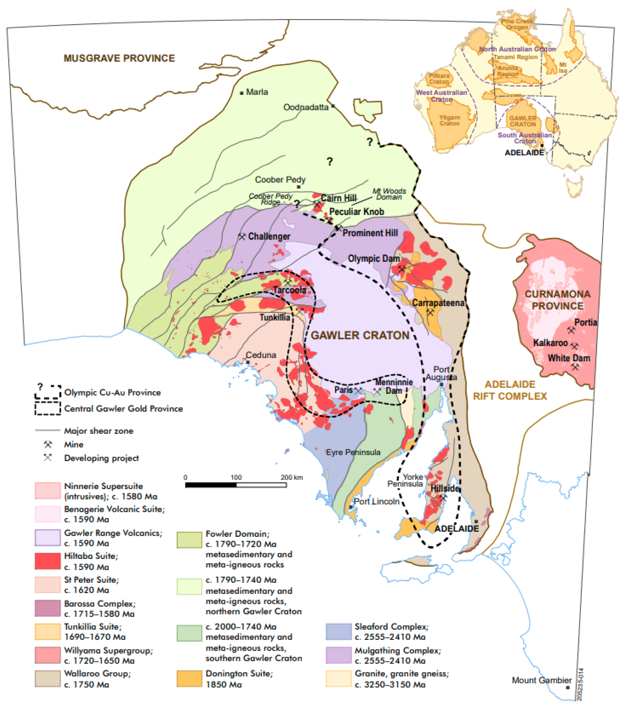
The Hillside Copper–Gold project is situated on the east coast of the Yorke peninsula in South Australia (
Figure 1) within the Central Gawler/Olympic Copper–Gold Province as defined by Skirrow et al. [
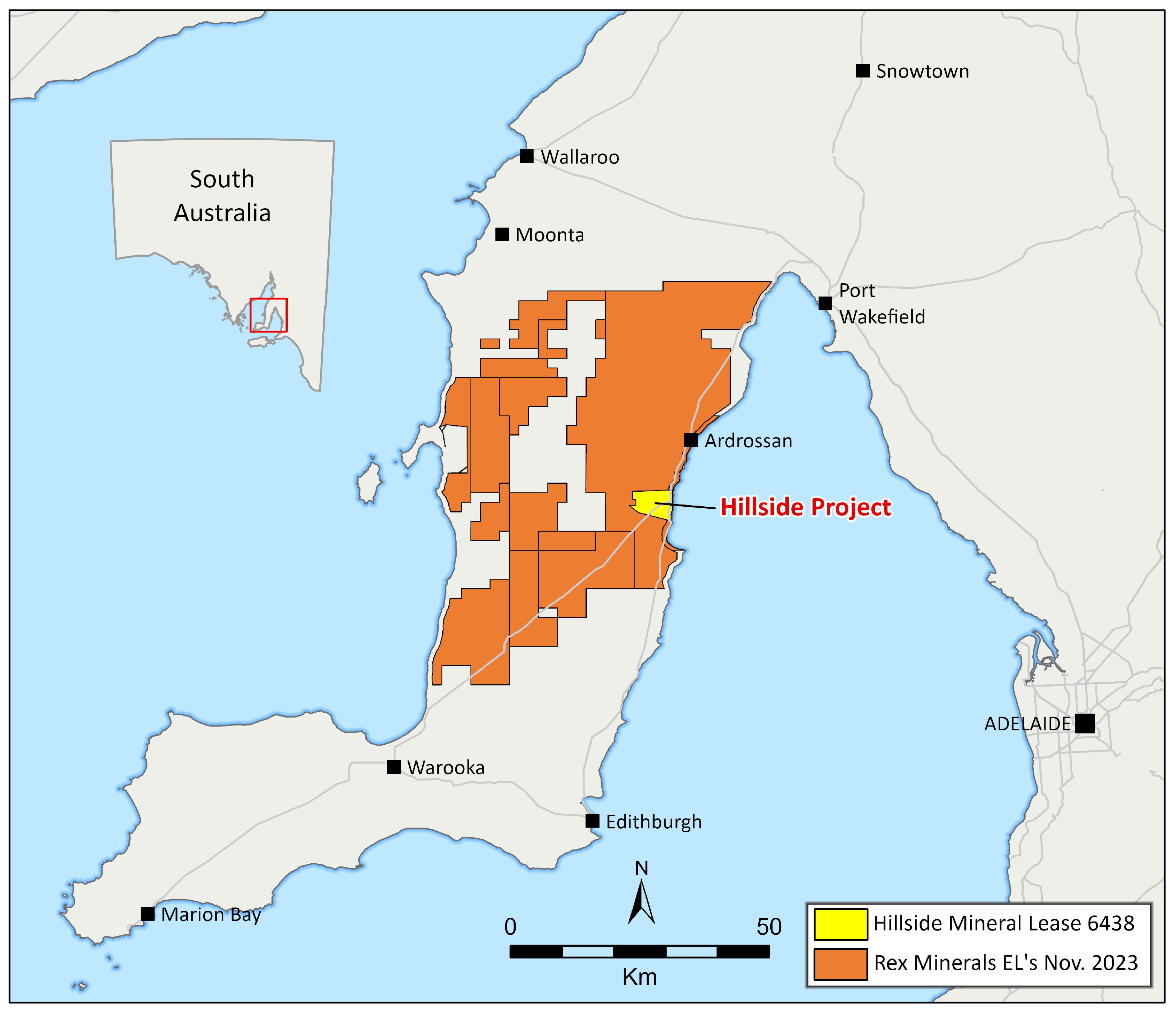
3]. The province hosts the major copper–gold deposits of the eastern Gawler craton including Olympic Dam, Carrapateena, and Prominent Hill. Mineral lease (ML 6438) (
Figure 2) encompasses the project area with Rex Minerals holding substantial exploration licences on the Yorke peninsula.
The Gawler craton is one of the most geologically significant regions in Australia. It is known for its complex and prolonged tectonic history that has created favourable conditions for ore formation; an exceptional example is Olympic Dam (
Figure 1), one of the world’s most abundant deposits of copper, gold, and uranium. While the Gawler craton holds substantial exploration potential, further discovery in the province will rely heavily on successful exploration under thick Neoproterozoic and Phanerozoic cover [
5].
The Hillside deposit was discovered in 2008 as a result of exploration drilling of discrete gravity and magnetic features which were in agreement with the regional structural trends [
6]. Gravity anomalies proved to be predominately mafic volcanic rocks of the Wallaroo Group. Early drilling intersected a major fault structure and recorded magnetite, garnet, and clinopyroxene with associated copper and gold mineralisation [
6].
Mineralisation and alteration at Hillside has been dated at approximately 1570 ± 8 Ma [
7,
8] and is therefore temporally related to the widespread intrusion of the Hiltaba suite and eruption of the Gawler Range volcanics. However, as with most major deposits in the Olympic Cu-Au province, the formational history is prolonged and complex involving multiple, likely discrete, mineralisation/remobilisation events. Of note are two recognised events: the Wartaken (1500–1450 Ma) and Coorabie (1470–1450 Ma) orogenies [
8].
The crustal scale Pine Point fault transecting through the region was reactivated during these events [
9] and movement along the fault likely would have encouraged the reactivation of smaller structures. Mineralising fluids may have utilised the decompressive and dilational conditions, allowing mineral precipitation where the physiochemical conditions permitted. As such, exploration should be focused along strike of the Pine Point fault and at intersections with secondary structures.
3. Materials and Methods
Ambient noise tomography (ANT) is a passive geophysical method that leverages the cross-correlation of random wavefields recorded at multiple seismic sensors to approximate Green’s functions. This effectively transforms each sensor into a virtual source and receiver from which phase delay information can be extracted and used to image the subsurface [
10,
11]. With a scientific history spanning over two decades, ANT has proven to be an effective tool for high-resolution imaging of geological structures beneath cover and at depth, e.g., [
12,
13,
14]. The method offers valuable information about the subsurface distribution of seismic velocity and is particularly advantageous due to the abundant presence of natural and anthropogenic seismic noise, making it a cost-effective and environmentally friendly technique. Recent advancements in seismic instrumentation and computational resources have further enhanced its potential.
Fleet Space Technologies (Fleet) has commercialised an ANT service named ExoSphere, utilising purpose-built real-time compact seismic nodes called Geodes. These Geodes offer increased sensitivity to low-frequency signals, reducing data gathering time compared to conventional nodal geophones [
15]. Fleet’s Geodes are equipped with a real-time direct-to-satellite Internet of Things (DtS-IoT) modem and edge processing capabilities, enabling rapid data transmission for cloud-based further processing. This breakthrough allows for unprecedented speed in subsurface imaging, thus accelerating the discovery of new mineral deposits [
15].
3.1. Data Collection
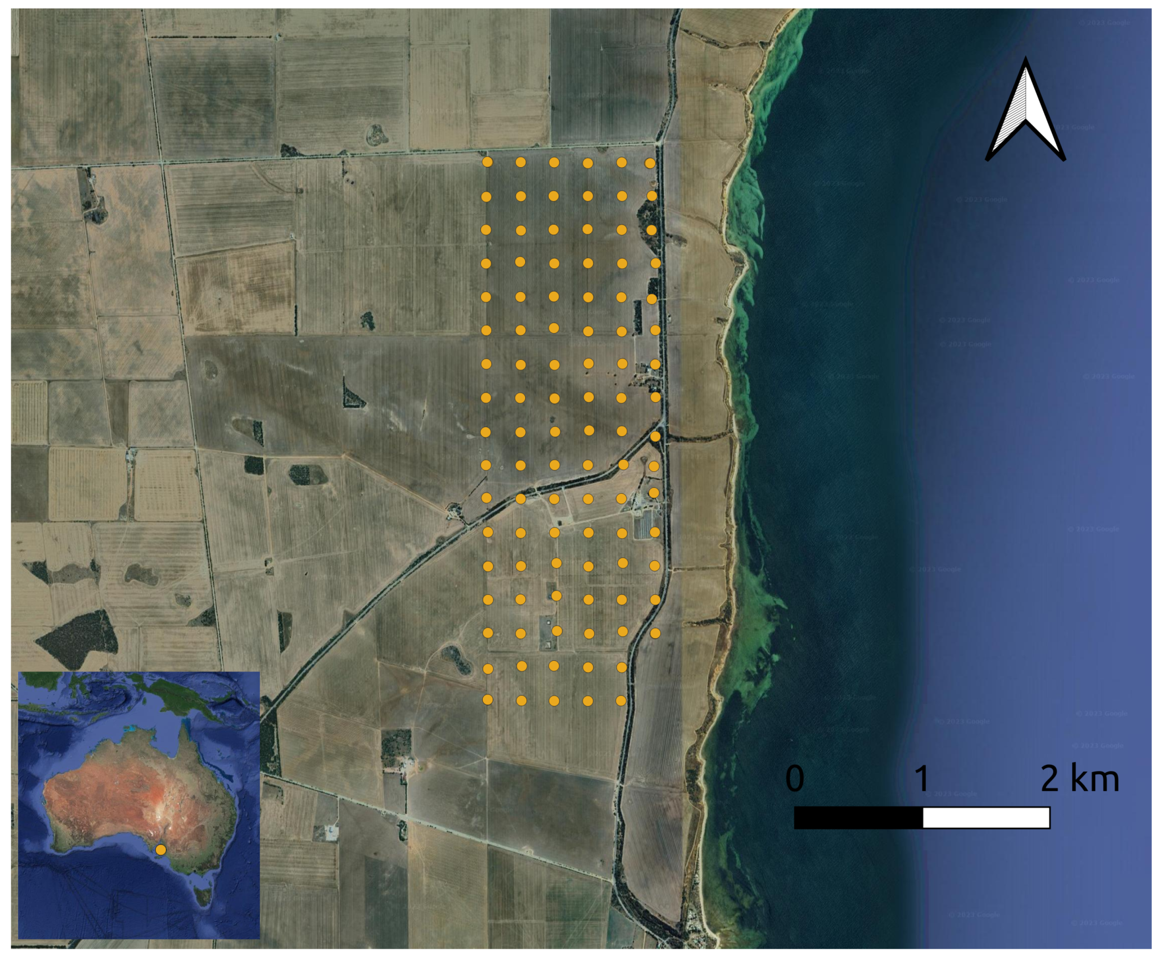
Fleet deployed a network of 100 Geodes with a specified spacing of 260 m, arranged in a 17 × 6 rectangular array (minus 2 from the SE corner), covering an area of approximately 5.5 km
2 for a duration of 14 days at the Hillside Copper Project (see
Figure 3). Continuous ambient seismic noise data was recorded at a 20 Hz sampling rate. Preceding transmission via satellite, the recorded data underwent whitening between 0.1 and 9 Hz to enhance the most pertinent frequencies. Additionally, one-bit normalisation was employed to down-weight the spectral response of transient signals, such as earthquakes, and significantly compress the data. The pre-processed data were promptly transmitted to the cloud for real-time processing, generating preliminary 3D models every 6 h. Throughout the deployment, consistent monitoring of data quality and Geode health was conducted via the ExoSphere portal to ensure a successful survey.
3.2. Further Data Processing
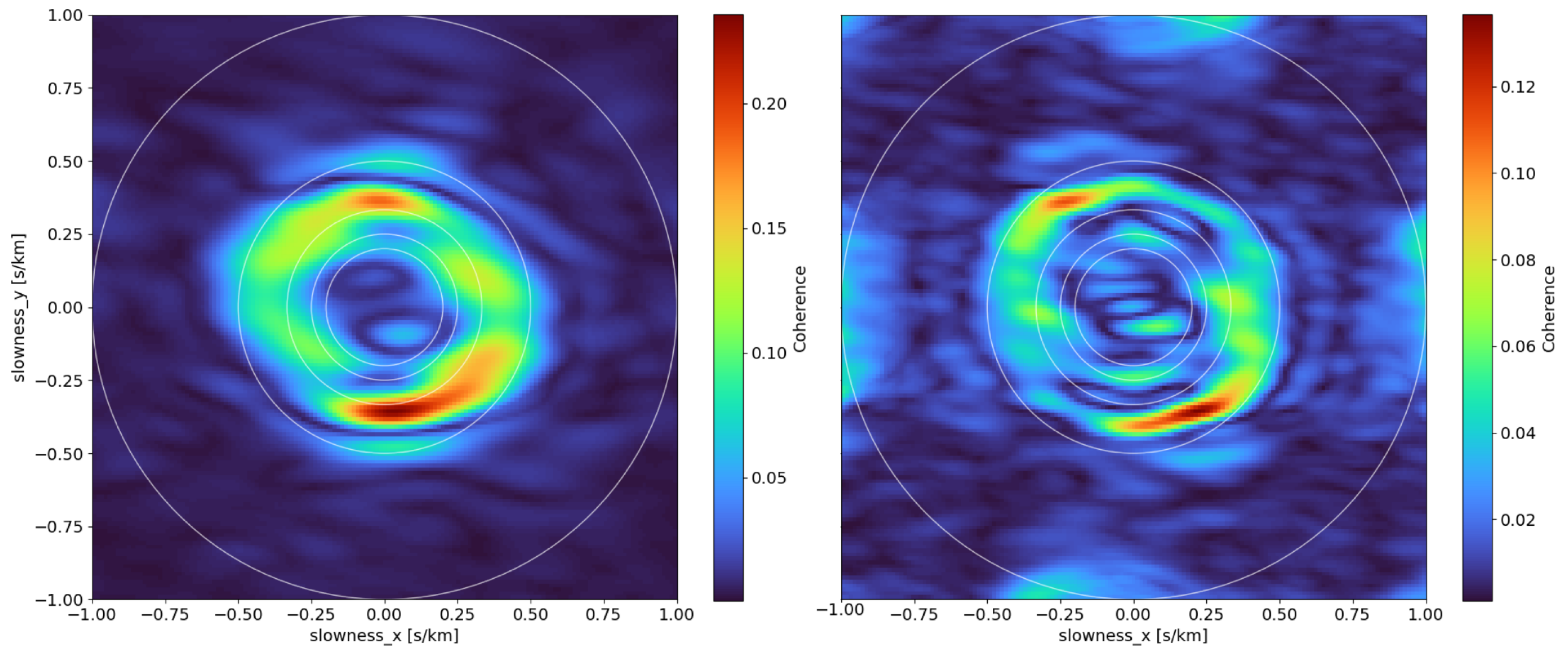
Directionality analysis of the ambient noise wavefield was performed using plane wave beamforming with a far field approximation to ascertain the primary noise sources at each frequency within the study area (
Figure 4) [
16]. Ideally, a uniform noise environment would exhibit evenly distributed beam power across all azimuths. The two images in
Figure 4 are for the frequency ranges 1.5–2.0 Hz (left) and 2.5–3.0 Hz (right). In both images the coherency of the ambient signal forms a circular pattern between the 2 km/s and 3 km/s velocity contours (white circles), indicating excellent noise distribution for the survey area. Given the frequency band recorded and by comparison of the circular pattern of directionality to the coastline (
Figure 2), the source of noise is inferred to be dominantly oceanic.
Following the method outlined by Bensen et al. [
17], the pre-processed ambient noise data underwent cross-correlation between unique pairs of sensors to calculate empirical Green’s functions, representing the subsurface response to ambient noise sources. The cross-correlation process involved measuring similarities and time delays in the received seismic signals, cancelling out incoherent signals while enhancing coherent seismic signals within the noise. The continuous noise records were divided into 20-minute segments to improve computational efficiency. For each station pair, the resulting cross-correlation functions were linearly stacked.
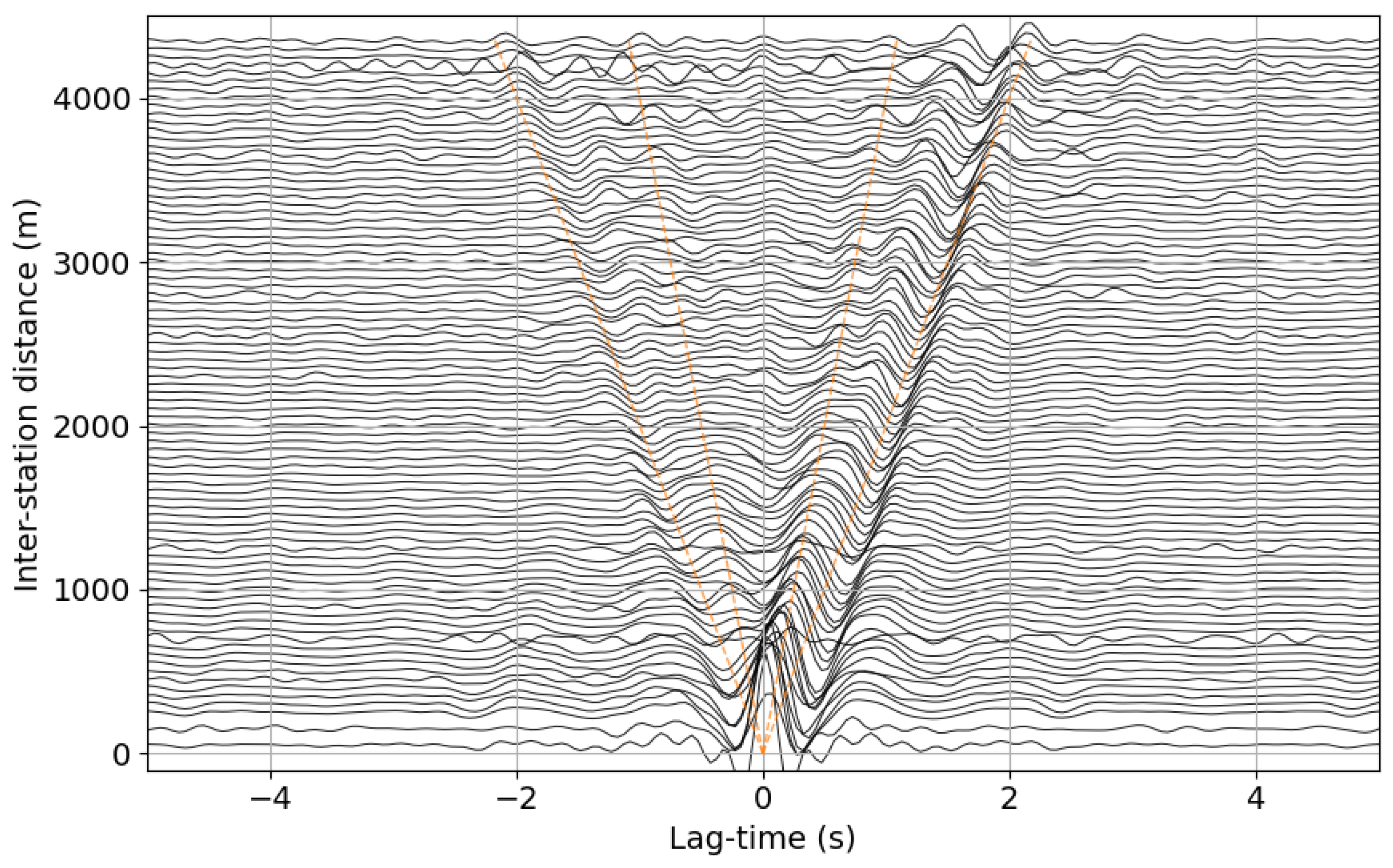
Figure 5 depicts a distinct ”V-shaped” moveout with high amplitude, indicating that ambient noise is arriving from all directions, and cross-correlations between Geode pairs are accurately recovered. To ensure the resulting model’s quality, we estimated the signal-to-noise ratio (SNR) of the cross-correlation functions (CCFs) between each Geode pair, removing low-SNR data from downstream processing.
The cross-correlation function (CCF) moveout plot illustrates the time-domain CCF for Geode pairs as a function of lag time and Geode pair, sorted by pair distance (
Figure 5). For two sensors, A and B, positive lags denote the travel time for a surface wave travelling from sensor A to sensor B, while negative lags indicate the reciprocal path. The moveout plot encompasses the full signal bandwidth. We see a clear moveout corresponding to Rayleigh waves with speeds between 2000 and 4000 m/s.
3.3. Dispersion Measurement
Surface waves exhibit dispersion, implying that lower frequencies sample greater depths, whereas higher frequencies sample shallower depths. This characteristic was exploited to extract phase velocity dispersion measurements at discrete frequencies from cross-correlation functions using two distinct methods: (1) fitting the real part of the Fourier transform of the correlation functions with a zero-order Bessel function of the first kind [
18,
19] and (2) automatic picking of dispersion curves on a frequency–time analysis (FTAN) image for each correlation function [
20,
21]. Generally, dispersion curves trend from higher phase velocities at low frequencies to lower phase velocities at higher frequencies, with variations linked to site geology. Outliers falling outside two standard deviations from the mean were identified and removed from downstream processing.
3.4. Three-Dimensional Model Development
We adopted the direct surface-wave tomography method by Fang et al. [
22] to simultaneously invert all dispersion measurements for 3D seismic velocity variations without frequency-dependent phase velocity maps. This method employed the 2D fast-marching technique of Rawlinson and Sambridge [
23] to compute surface wave travel times and ray paths between sources and receivers at each period, avoiding the assumption of great-circle path propagation. The sensitivity kernel matrix was constructed based on theoretical relationships between surface wave travel times, phase velocities, and layer variables, iteratively updated via the LSQR algorithm to achieve an optimal model by minimising differences between observed and predicted travel times calculated from the reference model across all frequencies. For a more comprehensive understanding of the inversion, please refer to Fang et al. [
22].
The 3D model space was parameterised with an isotropic cell size of 40 m and has dimensions 1450 m × 4300 m × 950 m. Surface elevations are corrected to a topographic grid with 10 m accuracy.
3.5. Temporal Stability of 3D Model
The convergence of the 3D model as a function of acquisition time is shown in
Figure 6. SNR plateaus at around 125 h of acquisition time while model RMS (%) plateaus at around 150 h. Traditionally, seismic sensors collecting ANT data at the exploration scale are left in the field for around 14 days. This conservatively long period follows the logic that collecting too much data is cheaper than collecting too little data. With real-time monitoring, we can extract the sensors at the peak of the SNR curve (or, implicitly, once collecting more data will have a negligible impact on the model). In the case of Hillside, the analysis presented in
Figure 6 shows that real-time monitoring reduces the acquisition time by 65%, from ∼14 days down to ∼5. This can save months of acquisition time when running multiple surveys to cover a large area.
3.6. Three-Dimensional Model Uncertainty
The uncertainty of 3D velocity structure, given the data, is based upon a hierarchy of errors from the various stages of the processing workflow, including: (i) variance of the stacked cross-correlation function, (ii) data fitting error, and (iii) the residual error and fitting variance from the least-squares optimisation method used to solve the direct inversion of dispersion measurements for 3D Vs structure. In this case study we do not make a specific analysis of model uncertainty or sensitivity, nor do we use numerical inverse methods which characterise the posterior probability distribution of the model parameters.
A useful approximation for the minimum bound on model uncertainty can be gained from 1D forward modelling of surface wave dispersion for a layered input model, where a sensitivity to Vs structure of ±10% for layer depth or velocity contrast can be assumed (e.g. Smith et al. [
24]). For a 3D case, we take the Geode spacing and array geometry into consideration and estimate a minimum uncertainty for layer depth or velocity of ±50 m from 0 to 500 m depth, and ±10% of depth from 500 m to max depth.
4. Results and Discussion
4.1. Velocity Structure of the Hillside Deposit and Setting
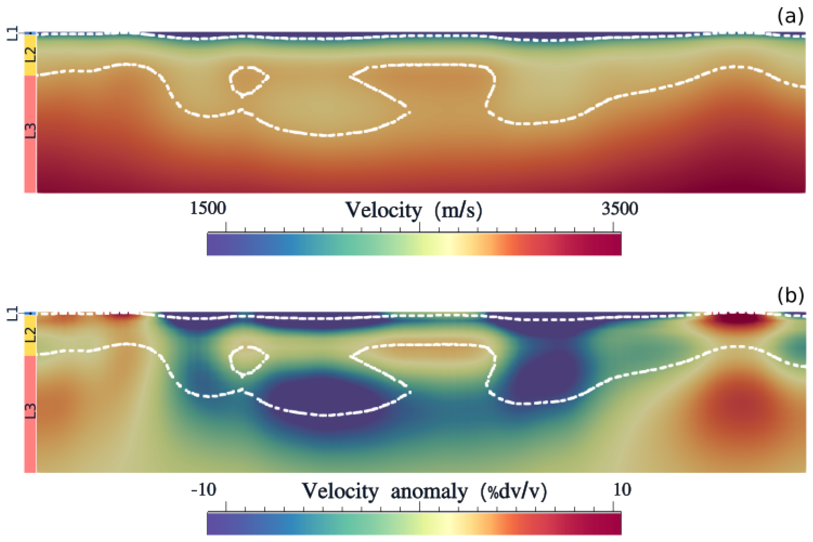
The ANT velocity model can be divided into three layers (
Figure 7). A cover layer of velocities less than 2000 m/s extends across the survey area and is confined to the first 80 m of the model. Based on previous drill core analysis, this layer generally coincides with a Tertiary cover sequence below or typical base of oxidation depths over the deposit through its thicker sections [
9]. The velocity transition below this layer is diffuse, especially to the east (
Figure 7a). This may reflect a heavily weathered basement but it should also be considered that the 4 Hz upper limit on coherent noise recorded for the survey limits sensitivity in the near-surface.
Below the cover sequence, two basement layers are resolved (
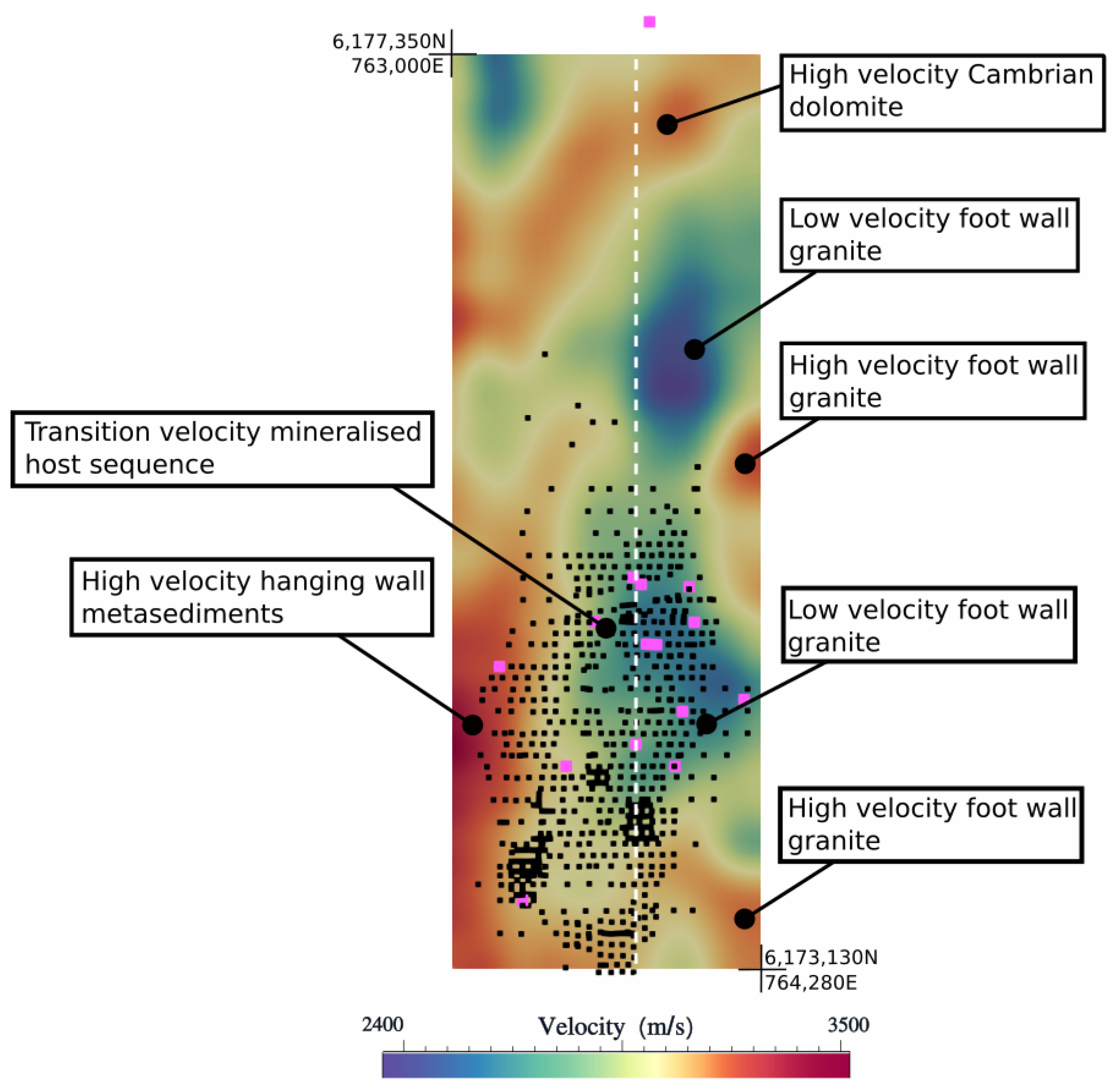
Figure 7). The upper basement layer shows strong lateral variation across the NS structure, jumping from an average of 2600 m/s in the east to 3200 m/s in the west. This velocity change marks the boundary between the hanging wall and the Point Pine Structural Corridor (PPSC) which hosts the mineralisation at Hillside (
Figure 8). The footwall to the east displays variable velocities which may be indicative of the observed irregular depth of weathering and structure. The PPSC sits within the velocity range of 2000–2800 m/s, increasing to the west. The upper basement layer thickens towards the middle of the model to approximately 675 m and thins to around 200 m in the north and south. The lower basement layer is characterised by velocities greater than 2800 m/s. Within this layer, the velocity contrast across the PPSC is diminished but remains low, relative to the bounding fault walls, and maintains its NS strike (
Figure 8).
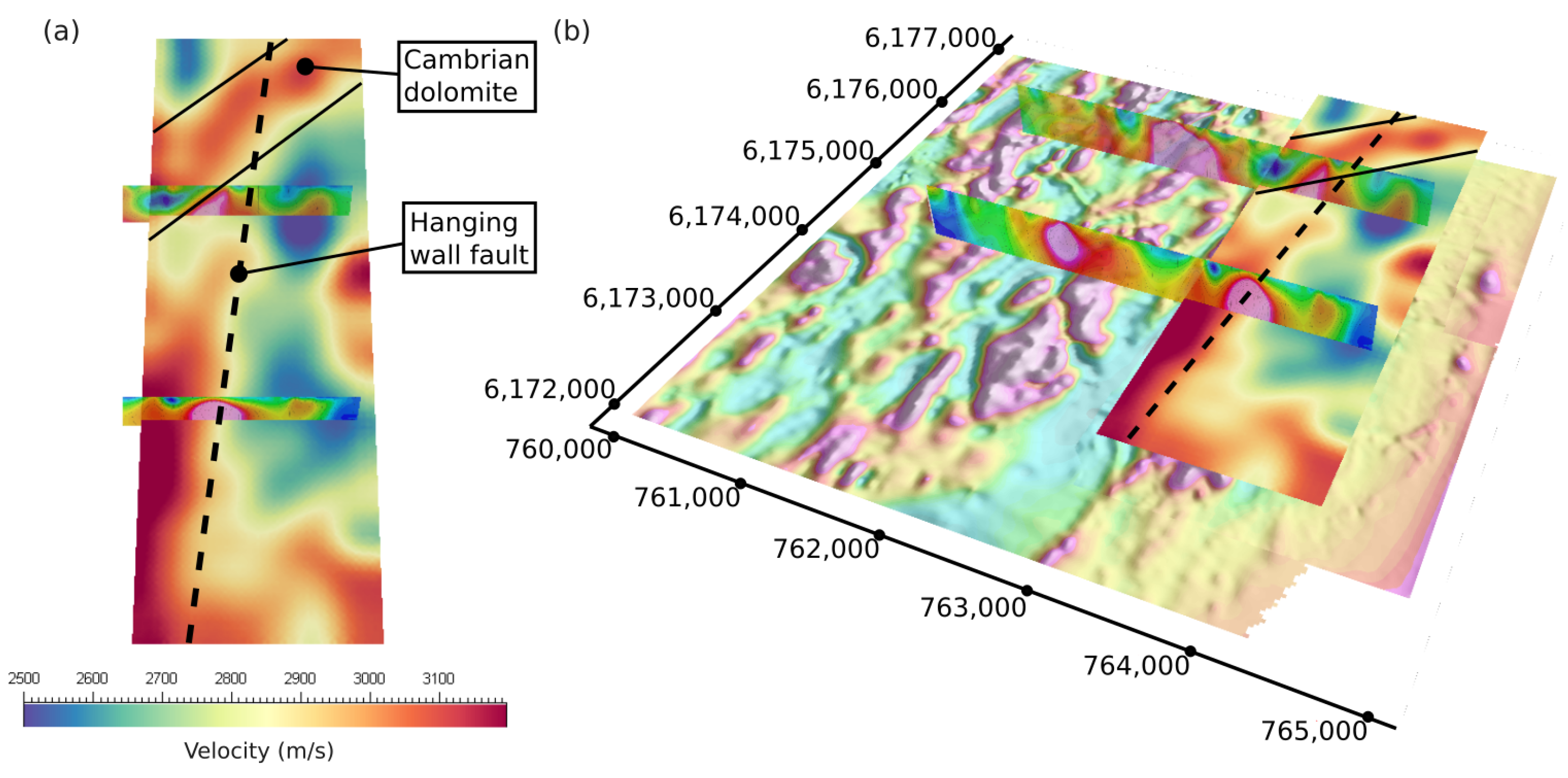
Beyond the mapped extent of the hillside deposit, to the north, a high velocity body striking NE cuts across the PPSC and into the footwall. This NE feature is interpreted to be the Cambrian dolomite basin based on a drilling intercept with hole HNDD-001, collared on the northern boundary of this survey along the strike of mineralisation. Its southern border is defined by a transition to the lower velocities of the PPSC (
Figure 8).
4.2. Comparison with Geological Model, Other Geophysical Data, and Drilling
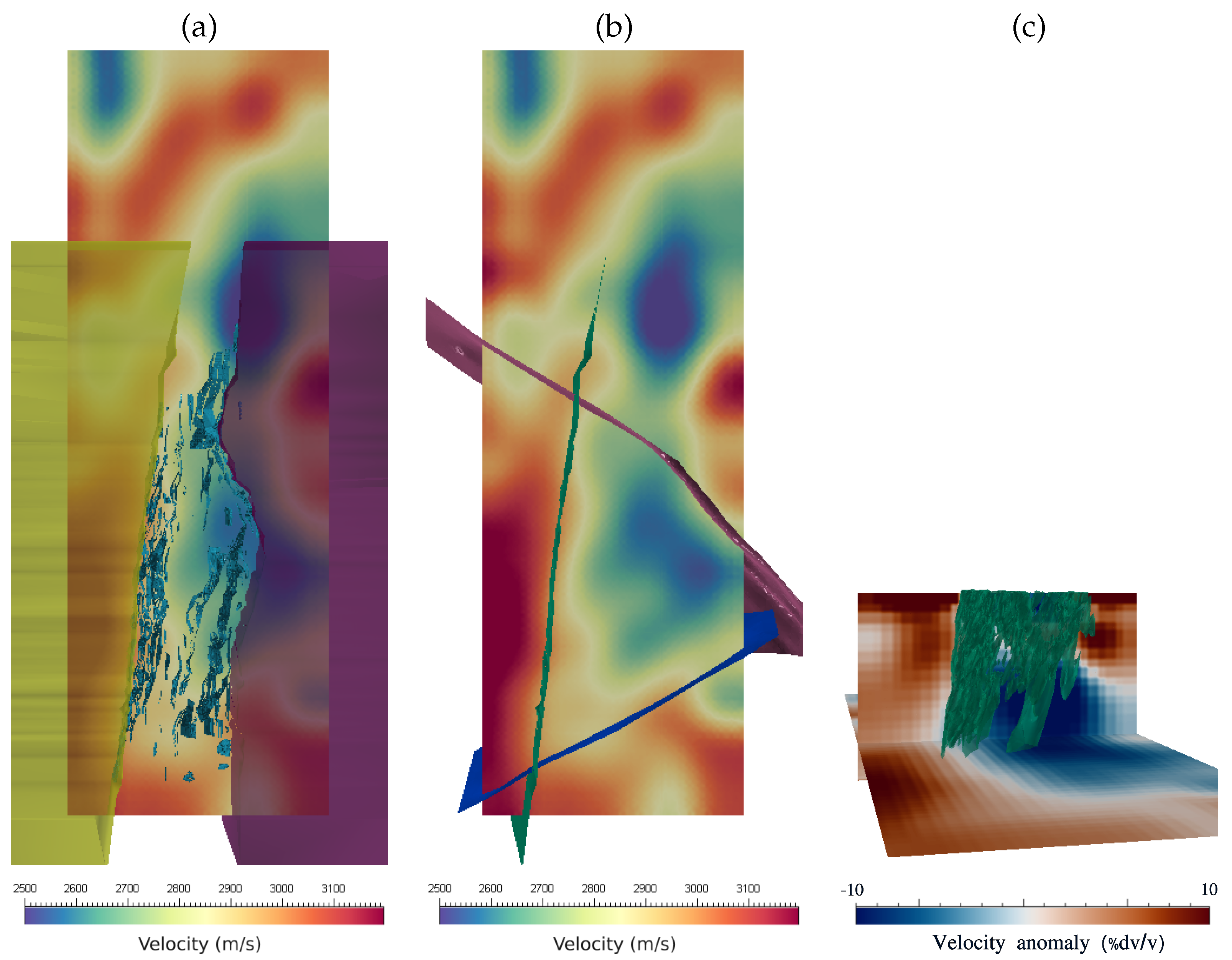
The relationship between the ANT volume and the Rex Minerals geological model is presented in
Figure 9a–c. The geological model can be categorised into three components: a hanging wall, a footwall, and a central, structurally complex zone that is defined as the PPSC. The hanging wall and footwall fault blocks, along with a 0.2% Cu mineralised shell, which sits within the PPSC, are shown against the ANT velocity model in
Figure 9a. The hanging wall is characterised by a velocity high running N–NNE, which, significantly, bounds the PPSC and forms a mineralised structural contact as part of the Hillside deposit. The footwall contact is diffuse by contrast and shows more velocity variation than the hanging wall contact. The PPSC exhibits the largest velocity range of the three, which results from an intermingling of lithologies, including skarns, metasediments, carbonates, and gabbro/syenite, some of which are heavily altered, brecciated, and mineralised.
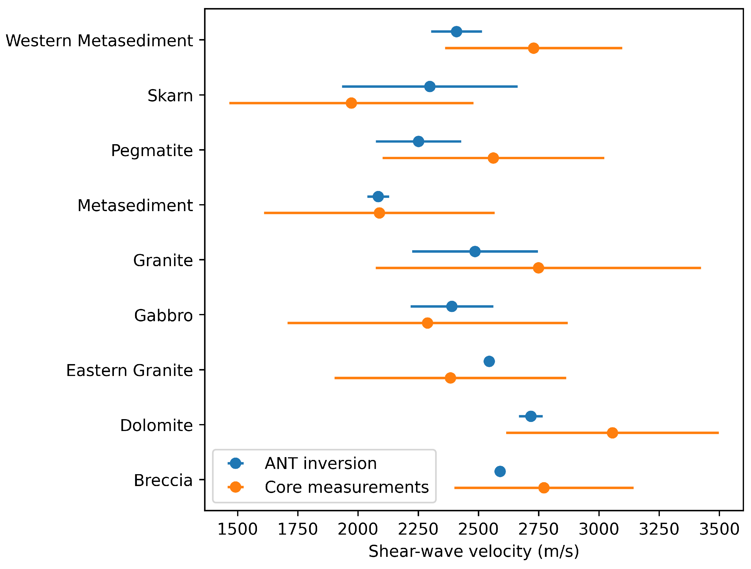
To provide empirical comparisons of diamond drill cores to the ANT velocity model, velocity measurements were taken on 75 samples from nine different rock types from the Hillside project using a handheld A1410 PULSAR—Ultrasonic pulse velocity measuring P-wave velocity (see
Table 1). The resulting velocity measurements are a reflection of rock density, porosity, ambient pressure, fractures, and other discontinuities. The measured P-wave velocities were converted to S-waves to enable comparison to the ANT model using the empirical relationship defined by Brocher [
25]. For every section of core for which handheld velocity measurements were taken, a value from the ANT velocity inversion was recorded for the same location. The results are plotted in
Figure 10 as an error bar plot, showing the mean and standard deviations for both the handheld velocity measurements and the ANT inversion velocities. A summary of the major features interpreted from this comparison are shown in
Figure 8.
Three major faults around the deposit are shown in
Figure 9b against the velocity model. The NS and NE trending faults lie at the edge of velocity highs. The NW structure lies at the edge of a velocity high to the east, cuts across the PPSC, and intercepts a velocity break (low) in the hanging wall to the west.
The location of modeled skarn against a cross-section of the velocity model is shown in
Figure 9c. To better highlight velocity variations at depth we subtract from every cell the mean velocity for its depth and normalise the difference to the mean, removing the increase in velocity due to pressure. The observed variations are then the velocity anomaly (% dv/v) about a mean value.
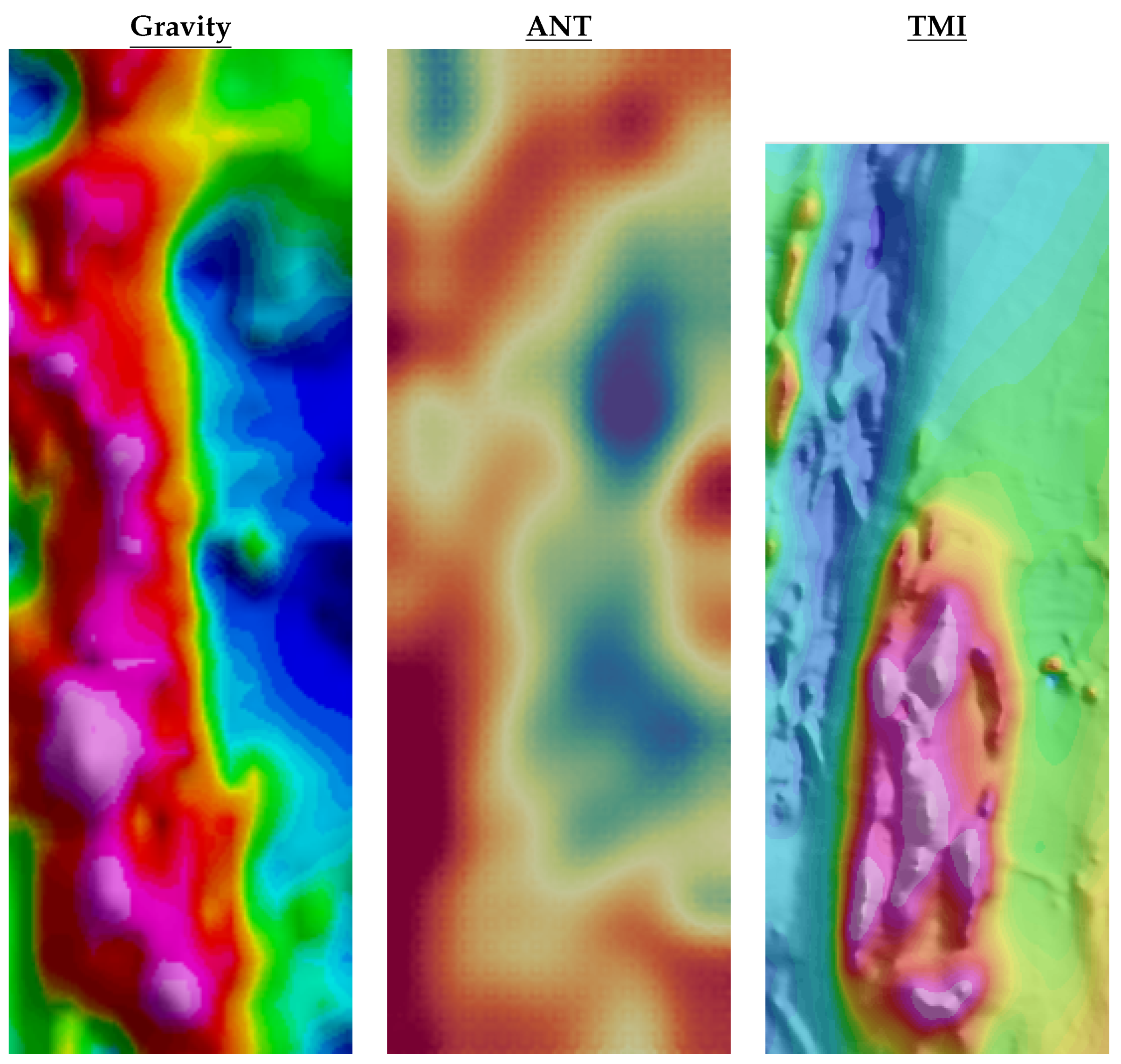
The ANT velocity model is in broad agreement with existing grids of magnetic and gravity data. The magnetic data delineates the Hillside host rocks and was targeted in the preliminary exploration. All three techniques image the NS fabric that defines the geology of the region (
Figure 11). In detail, the ANT data aligns better with the total magnetic intensity (TMI) data, which maps the subtle N–S strike of the PPSC. In both datasets, the western hanging wall fault boundary is the clearest expression of this trend. In contrast, the gravity data are dominated by an elongated gravity high that runs N–NW, cutting through the PPSC and the hanging wall fault. The known extent of the Hillside orebody coincides roughly with a local peak in TMI (orange to pink colours). A similar magnetic anomaly can be seen ∼1 km west of the deposit (see the first vertical derivative of TMI shown in
Figure 12b). The magnetic anomaly does not extend to the north of the deposit area but the velocity model shows strong continuity and may indicate a possible deposit extension of the deposit below thicker cover.
The ANT velocity model has an additional geophysical correlate in previously collected induced polarisation data. Two distinct peaks in chargeability coincide with key structures highlighted by the ANT velocity model (
Figure 12a). The first lies across the boundary of the velocity high that maps the hanging wall fault, coincident with high-grade Cu mineralisation. The second lies across the newly discovered NE high velocity feature, interpreted to be Cambrian Dolomite, just north of the main deposit. The black dashed lines highlight the strike of the hanging wall fault and the solid black lines bound the interpreted Dolomite. Tracing the NE strike of the dolomite SW, outside the ANT survey area it intersects another chargeability anomaly of the same magnitude as the two over the ANT survey region (
Figure 12b). In addition, the structure cuts a major magnetic high with similar geometry and magnitude to the magnetic anomaly that defines the extent of the main Hillside deposit (
Figure 11).
4.3. Future Exploration at Hillside Confirmed by ANT Results
The Fleet 3D ANT velocity model successfully images known structures, lithological domains, and the cover-basement contact. Beyond the well-surveyed deposit extent, two areas of interest have been confirmed for future exploration: one to the north and one to the west of the known Hillside deposit.
The area of interest to the north is a continuation of the velocity anomaly associated with the mineralised zone. The velocity anomaly increases in amplitude to the north, below thickening cover, before cutting through a newly interpreted Cambrian dolomite unit. The interpreted dolomite unit occurs along a transition from high velocities in the north to low velocities in the south. As with mineralisation along the PPSC, the dolomite body coincides with a chargeability high.
The area of interest to the west represents an extension of the dolomite unit to the SW. It can be traced outside the ANT survey following a magnetic lineament in the 1VD of TMI. Approximately one kilometre west of the ANT survey, the magnetic break intercepts an area mimicking two geophysical characteristics of the known Hillside deposit: a chargeability high at the edge of a large NS trending magnetic anomaly.
5. Conclusions
In this paper, we demonstrate the efficacy of ambient noise tomography (ANT) in the geophysical exploration of the Hillside Iron Oxide–Copper–Gold (IOCG) deposit within the Gawler Craton, South Australia. We have shown that the ANT method accurately captures the structural framework of the Hillside IOCG down to one kilometre, proving a resolving power at depth unmatched by the existing potential field and EM datasets. In particular, ANT overcomes two central issues with potential field data: the inverse-power decay limiting resolution undercover and the non-uniqueness of depth-to-source estimates.
Furthermore, integrating ANT with other geophysical datasets, such as Total Magnetic Intensity (TMI) and gravity surveys, offers a multi-faceted view of the subsurface structures and distribution of the mineralised host lithology. Robust depth information gathered from the ANT velocity models could be used to constrain inverse or forward modelling of these potential field datasets, enhancing the accuracy of the most commonly applied geophysical techniques in IOCG exploration.
One of the most significant outcomes of this research is the confirmation of areas for future exploration. The ANT data suggests potential extensions of the Hillside deposit to the north and west. These findings not only open up complimentary avenues for resource expansion at the Hillside project but also exemplify the potential of ANT in exploring similar IOCG systems.
The implications of this research extend beyond the specific context of the Hillside deposit. The demonstrated effectiveness of ANT in this study suggests a broader applicability for the exploration of IOCG deposits where structure is a controlling factor in mineralisation, where cover hinders near-surface techniques, and particularly where steeply dipping geology escapes imaging by reflection seismic techniques.
Author Contributions
Conceptualisation, T.J. and G.O.; methodology, G.O. and M.G.; software, G.O., M.G. and N.S.; validation, T.J., N.S., G.O., B.M., L.C., C.W. and S.O.; formal analysis: T.J., N.S., G.O., M.G., B.M., L.C., C.W. and S.O.; data curation, T.J. and N.S.; writing—original draft preparation, T.J., G.O. and B.M.; writing—review and editing, T.J., B.M., B.N., N.S., L.C., C.W., D.B. and S.O.; visualisation, T.J., G.O. and B.M. All authors have read and agreed to the published version of the manuscript.
Funding
This research received no external funding.
Data Availability Statement
Restrictions apply to the availability of these data. Data were obtained for mineral exploration and their public release will accord with the provisions of the Mining Act 1971 and Mining regulations 2020.
Acknowledgments
The authors would like to thank the following: Rex Minerals for their collaborative spirit throughout this project. Without their generous sharing of knowledge, data, and time this work could not have been possible. Fleet staff who supported this work, from the development of ExoSphere and the Geode from the ground up, to managing the deployment and data delivery. And the field crew, for getting their hands dirty to carefully and rapidly collect a high-quality dataset.
Conflicts of Interest
The authors declare no conflicts of interest.
References
- Funk, C. Geophysical vectors to IOCG mineralisation in the Gawler Craton. ASEG Ext. Abstr. 2013, 2013, 1–5. [Google Scholar] [CrossRef]
- Okan, E.O. Feasibility of Using Regional Seismic Reflections Surveys to Discover Iron Oxide Copper Gold (IOCG) Deposits in the Gawler Craton, South Australia. Ph.D. Thesis, Curtin University, Singapore, 2018. [Google Scholar]
- Skirrow, R.; Bastrakov, E.; Davidson, G.; Raymond, O.; Heithersay, P. The geological framework, distribution and controls of Fe-oxide Cu-Au mineralisation in the Gawler Craton, South Australia. Part II-alteration and mineralisation. In Hydrothermal Iron Oxide Copper-Gold & Related Deposits: A Global Perspective; PGC Publishing: Toronto, ON, Canada, 2002; Volume 2, pp. 33–47. [Google Scholar]
- Gum, J. Gold mineral systems and exploration, Gawler Craton, South Australia. MESA J. 2019, 3, 51–65. [Google Scholar]
- Reid, A. The Olympic Cu-Au Province, Gawler Craton: A Review of the Lithospheric Architecture, Geodynamic Setting, Alteration Systems, Cover Successions and Prospectivity. Minerals 2019, 9, 371. [Google Scholar] [CrossRef]
- Teale, G.; Say, P.; Green, N.; Forgan, H.; Went, C.; Cole, L. Rare earths and other trace elements in minerals from skarn assemblages, Hillside iron oxide-copper-gold deposit, Yorke Peninsula, South Australia. Lithos 2014, 184, 456–477. [Google Scholar]
- Conor, C.; Raymond, O.; Baker, T.; Teale, G.; Say, P.; Lowe, G.; Porter, T. Alteration and mineralisation in the Moonta-Wallaroo copper-gold mining field region, Olympic Domain, South Australia. Hydrothermal Iron Oxide-Copp.-Gold Relat. Depos. Glob. Perspect. 2010, 3, 147–170. [Google Scholar]
- Thompson, C. Thermal and Exhumation History of the Central Yorke Peninsula, Southern Gawler Craton. Honours Thesis, University of Adelaide, Adelaide, SA, USA, 2013. Available online: https://digital.library.adelaide.edu.au/dspace/bitstream/2440/106460/2/02wholeGeoHon.pdf (accessed on 11 December 2023).
- Ismail, R. Spatial-Temporal Evolution of Skarn Alteration in IOCG Systems: Evidence from Petrography, Mineral Trace Element Signatures and Fluid Inclusion Studies at Hillside, Yorke Peninsula, South Australia. Ph.D. Thesis, University of Adelaide, Adelaide, SA, USA, 2015. Available online: https://digital.library.adelaide.edu.au/dspace/handle/2440/112582 (accessed on 11 December 2023).
- Lobkis, O.I.; Weaver, R.L. On the emergence of the Green’s function in the correlations of a diffuse field. J. Acoust. Soc. Am. 2001, 110, 3011–3017. [Google Scholar] [CrossRef]
- Snieder, R. Extracting the Green’s function from the correlation of coda waves: A derivation based on stationary phase. Phys. Rev. E 2004, 69, 046610. [Google Scholar] [CrossRef] [PubMed]
- Shapiro, N.M.; Campillo, M.; Stehly, L.; Ritzwoller, M.H. High-resolution surface-wave tomography from ambient seismic noise. Science 2005, 307, 1615–1618. [Google Scholar] [CrossRef] [PubMed]
- O’Donnell, J.; Thiel, S.; Robertson, K.; Gorbatov, A.; Eakin, C. Using seismic tomography to inform mineral exploration in South Australia: The AusArray SA broadband seismic array. MESA J. 2020, 93, 24–31. [Google Scholar]
- Chen, S.; Gao, R.; Lu, Z.; Liang, Y.; Cai, W.; Cao, L.; Chen, Z.; Wang, G. Shear wave velocity structure of the upper crust in north Xiaojiang fault zone in SE Tibet via short-period ambient noise dense seismic array. Phys. Earth Planet. Inter. 2023, 344, 107110. [Google Scholar] [CrossRef]
- Olivier, G.; Borg, B.; Trevor, L.; Combeau, B.; Dales, P.; Gordon, J.; Chaurasia, H.; Pearson, M. Fleet’s geode: A breakthrough sensor for real-time ambient seismic noise tomography over DtS-IoT. Sensors 2022, 22, 8372. [Google Scholar] [CrossRef] [PubMed]
- Gal, M.; Reading, A.M. Beamforming and polarisation analysis. In Seismic Ambient Noise; Cambridge University Press: Cambridge, UK, 2019; pp. 32–72. [Google Scholar]
- Bensen, G.; Ritzwoller, M.; Barmin, M.; Levshin, A.L.; Lin, F.; Moschetti, M.; Shapiro, N.; Yang, Y. Processing seismic ambient noise data to obtain reliable broad-band surface wave dispersion measurements. Geophys. J. Int. 2007, 169, 1239–1260. [Google Scholar] [CrossRef]
- Aki, K. Space and time spectra of stationary stochastic waves, with special reference to microtremors. Bull. Earthq. Res. Inst. 1957, 35, 415–456. [Google Scholar]
- Ekström, G.; Abers, G.A.; Webb, S.C. Determination of surface-wave phase velocities across USArray from noise and Aki’s spectral formulation. Geophys. Res. Lett. 2009, 36, 1–5. [Google Scholar] [CrossRef]
- Levshin, A.L.; Pisarenko, V.F.; Pogrebinsky, G.A. On a frequency-time analysis of oscillations. Ann. Geophys. 1972, 28, 211–218. [Google Scholar]
- Luo, Y.; Yang, Y.; Xu, Y.; Xu, H.; Zhao, K.; Wang, K. On the limitations of interstation distances in ambient noise tomography. Geophys. J. Int. 2015, 201, 652–661. [Google Scholar] [CrossRef]
- Fang, H.; Yao, H.; Zhang, H.; Huang, Y.C.; van der Hilst, R.D. Direct inversion of surface wave dispersion for three-dimensional shallow crustal structure based on ray tracing: Methodology and application. Geophys. J. Int. 2015, 201, 1251–1263. [Google Scholar] [CrossRef]
- Rawlinson, N.; Sambridge, M. Wave front evolution in strongly heterogeneous layered media using the fast marching method. Geophys. J. Int. 2004, 156, 631–647. [Google Scholar] [CrossRef]
- Smith, N.R.A.; Reading, A.M.; Asten, M.W.; Funk, C.W. Constraining depth to basement for mineral exploration using microtremor: A demonstration study from remote inland Australia. Geophysics 2013, 78, B227–B242. [Google Scholar] [CrossRef]
- Brocher, T.M. Empirical relations between elastic wavespeeds and density in the Earth’s crust. Bull. Seismol. Soc. Am. 2005, 95, 2081–2092. [Google Scholar] [CrossRef]
| Disclaimer/Publisher’s Note: The statements, opinions and data contained in all publications are solely those of the individual author(s) and contributor(s) and not of MDPI and/or the editor(s). MDPI and/or the editor(s) disclaim responsibility for any injury to people or property resulting from any ideas, methods, instructions or products referred to in the content. |
© 2024 by the authors. Licensee MDPI, Basel, Switzerland. This article is an open access article distributed under the terms and conditions of the Creative Commons Attribution (CC BY) license (https://creativecommons.org/licenses/by/4.0/).


 ,
, 


