
Kinematic Modeling with Experimental Validation of a KUKA®–Kinova® Holonomic Mobile Manipulator

Faculty of Electronics and Automation, Technical University—Sofia, Plovdiv Branch, 4000 Plovdiv, Bulgaria
*
Author to whom correspondence should be addressed.
Electronics 2024, 13(8), 1534; https://doi.org/10.3390/electronics13081534
Submission received: 15 January 2024
/
Revised: 3 April 2024
/
Accepted: 11 April 2024
/
Published: 17 April 2024
(This article belongs to the Special Issue Recent Advances in Modelling, Control and Navigation of Ground and Aerial Robots)
Abstract
:We have proposed an open-source holonomic mobile manipulator composed of the KUKA youBot holonomic mobile platform with four Swedish wheels and a stationary aboard six-degrees-of-freedom Kinova Jaco Gen 2H manipulator, and we have developed corresponding kinematic problems. We have defined forward and inverse analytic Jacobians and designed Jacobian algorithms of forward and inverse mobile manipulator kinematics. An experimental test conducted with the designed laboratory prototype of the investigated mobile manipulator with the described kinematics was used to verify the obtained theoretical results. The goal of the test was to keep constant the position of the gripper in 3D space while the mobile platform is moving to some extend in the 2D workspace.
1. Introduction
In the present day, robots with various configurations (mobile robots, robot manipulators, mobile manipulators, etc.) are very rapidly advancing in performing different application tasks in our everyday lives. There are also many companies that offer on the market service robots dedicated to helping disabled people in their daily activities. Currently, various approaches for human–robot interactions are gaining popularity, including, for example, manual guidance, among others. It should be noted that such machines, especially in their recently investigated collaborative implementation, must correspond to the safety standards developed in the EU [1,2,3]. The widespread use of robots also requires a high level of understanding of the problems involved into this field of science [4,5,6,7,8]. In the present work, we describe existing research into the mathematical modeling of the kinematics of a holonomic mobile manipulator that has remarkable mobility and handling capabilities. The combined machinery contains two devices: a mobile platform and a 6 DoF manipulator. The chosen mobile platform, KUKA youBot, has four omnidirectional wheels, and it is widely used for scientific research tasks [9]. Installed on the top of the mobile platform robot manipulator, Kinova Jaco Gen2 is often used to assist disabled people by helping them with their daily activities, such as drinking water, holding a spoon, etc. The manipulator has also been selected for the experiments because it is supported by numerous software tools that make its control open to users and provide an opportunity to explore different control approaches. Such a combination of mobile platforms and manipulators widens the fields of application of the resulting mobile manipulators. Examples of similar assemblies can be found in [10,11,12]. All those efforts aimed to extend the working space of manipulators. However, the assembly of a mobile platform and a manipulator requires relevant kinematic models. An interesting solution can be found in [13], where authors present a configuration of a mobile manipulator based on Boston Dynamics Spot that is additionally equipped with a robotic arm. Some of the mobile manipulators with open-chain kinematics have been studied and are presented in [14,15,16,17,18,19,20]. More recent studies on the inverse kinematics frameworks of mobile manipulators are given in [21,22,23,24].
In the present work, we derive the forward kinematics, inverse kinematics, Jacobian and inverse Jacobian of the investigated mobile manipulator. The obtained mathematical models are then applied to control the movement of the laboratory prototype mobile manipulator in the task of maintaining a constant position and orientation of the manipulator’s end-effector in 3D space while the mobile platform is moving to some extent in the 2D workspace. This is achieved by controlling the speed of each mobile manipulator link and the speed of each mobile platform wheel. Afterwards, the efficacy of the proposed approach is evaluated by running a real-world experiment.
The article is structured in the following way: In Section 2, we describe the components of the mobile manipulator and derive their kinematic models. Then, the forward and inverse kinematics of the mobile manipulator and Jacobian algorithms are derived. In Section 3, the achieved results from the conducted experimental test carried out with the constructed laboratory prototype are presented. Section 4 contains conclusions.
2. Devices and Mathematical Models
2.1. The Mobile Manipulator
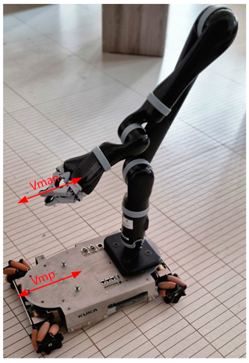
The assembled structure consists of two essential devices: a holonomic mobile platform and a six-degrees-of-freedom (6 DoF) robot manipulator (Figure 1). The mobile platform is a KUKA youBot holonomic platform, and the implemented spherical wrist robot is a Jaco Gen2 manipulator produced by the Canadian company Kinova.
This paper discusses the mathematical derivation of many important aspects that are related to the designed mobile manipulator: the forward and inverse kinematics of the mobile platform, forward and inverse kinematics of the manipulator Jaco Gen2, combined homogeneous transformation between the mobile platform and the end-effector, manipulator’s Jacobian matrix, manipulator’s inverse Jacobian matrix, and synchronization between the velocities of these two individual components. The obtained theoretical results have been verified via the conducted experimental test using a laboratory prototype of the above mobile manipulator. The implemented control software of the prototype uses ROS Melodic (Robot Operating System)-implemented packages, which were either provided by the manufacturers of the devices or are freely available from the web. The transfer of the control signals and feedback values is provided by the ROS’s topics, the ROS’s actions, and the ROS’s services. Each one of these types of communication is used depending on the existing situation. The presented results show the velocities of the mobile platform and the robot manipulator . These velocities allow for achieving a stable positioning of the end-effector during a movement of the mobile platform. The resulting velocity is .
2.2. The Mobile Platform KUKA youBot
The KUKA youBot mobile platform gives us the opportunity to expand the working space of the manipulator. Thus, the proposed structure of mobile manipulator enhances its functionalities.
However, in the design, this combination also increases the complexity of the whole robot system structure while increasing the mobile robot’s own weight and energy consumption. In order to complete complex work, the manipulator and omnidirectional vehicle must be in perfect harmony, and they also need to reduce energy loss. Therefore, the study of omnidirectional mobile operating robot has important theoretical and practical value.
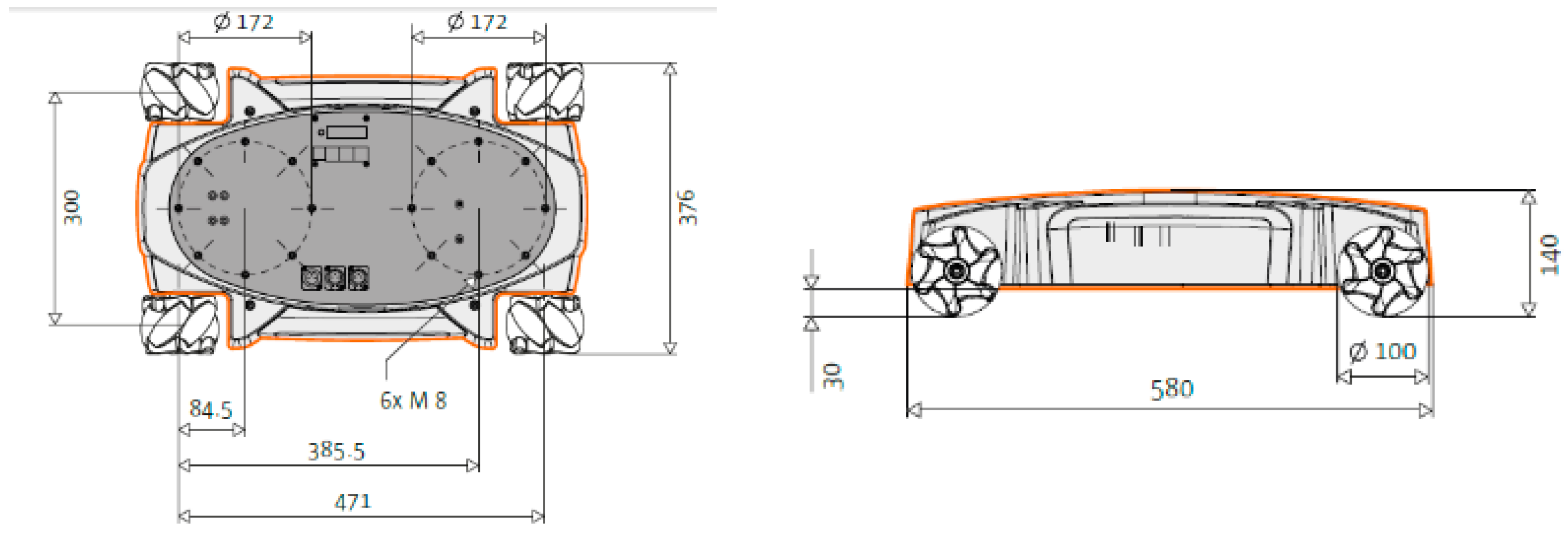
The next figure (Figure 2) shows the most significant dimensions of the KUKA youBot mobile platform and its structure.
The mobile platform is controlled by an onboard computer with embedded Intel Atom dual-core CPU and 2 GB RAM, 32 GB SSD, WLAN and a USB interface. Available interfaces are USB and EtherCAT/Ethernet. The existing WiFi connection makes possible the establishment of ROS communication.
The conventional approach for description of the motion of the mobile platform in a 2D plane requires the definition of coordinate frames. To specify the position and the orientation of the mobile platform onto the plane, we have to establish a relationship between the reference frame of the plane and the local frame of the platform. The axes and define an arbitrary inertial basis on the plane as the global reference frame from some origin . To indicate the position and orientation of the mobile platform, we choose a geometric center of the platform chassis-point P, and, thus, it is the origin of the platform’s local reference frame. The axes define the mobile platform’s local reference frame. The column vector (2) specifies the position and the orientation of the platform local reference frame in the global reference frame [25,26]:
where x and y are the displacements along the axis and axis, and the orientation is defined by .
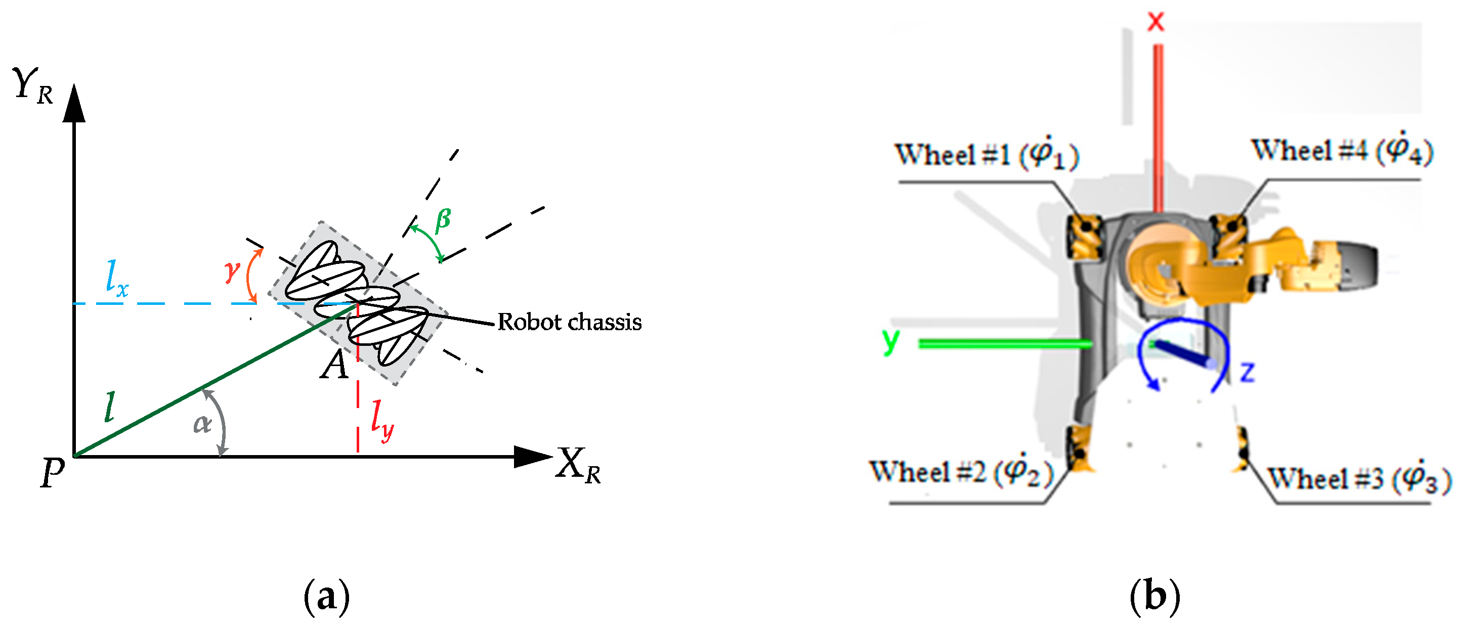
The KUKA youBot mobile robotic platform is controlled by varying the rotational speed of each of its omnidirectional wheels (Figure 3b).
The kinematic model describes the relationship between the rotational speeds of the four wheels , , and and the speed of the mobile platform in the 2D plane. The types of wheels and robot chassis geometry define this relationship. Each wheel introduces a set of mathematical constraints on the movement of the platform.
According to [25], using the constraints, we can obtain the kinematic model of the mobile robot. For a Swedish (mecanum) wheel, the following equations must be satisfied [25,26]:
where V1 and V2 denote the following three-element vectors:
the matrix R is the rotational matrix, and r denotes the radius of the wheels.
The index denotes the number of platform wheels.
Considering the construction parameters of the platform: the length , , (the robot dimensions are shown in (Figure 2) and the notations in (Figure 3a)), the angles and can be calculated according to the following equations [26]:
where, for the considered platform, and .
According to the theory of kinematics of the Swedish wheel [25], and considering the fact that the axes of the four wheels are perpendicular to PXR, then using the notations in Figure 3a, it is possible to express the angle and the length :
Table 1 contains the kinematic parameters of the mobile platform.
The forward kinematics of the mobile platform is described by the following matrix equation [26]:
And the inverse kinematic model is
2.3. The Manipulator KINOVA Jaco Gen 2
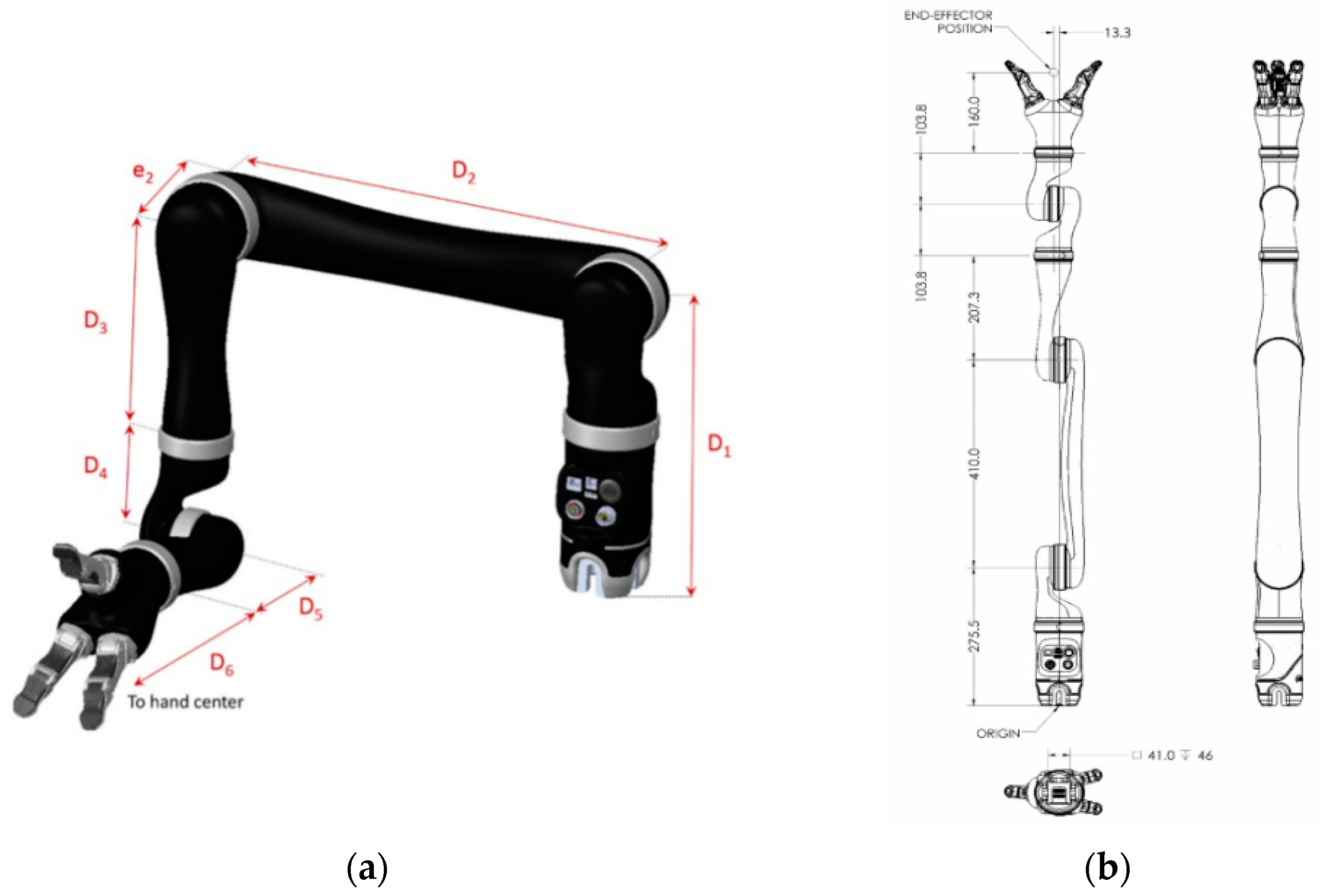
The geometric dimensions are shown in Table 2; these values are essential components of forward kinematics and notations: are structural elements of the homogeneous transformations.
In Table 3, some physical characteristics of the manipulator Jaco Gen2 Spherical Wrist are given.
Kinova Jaco Gen2 has specifically designed actuators mechanics and electronics. They use DC brushless motors with harmonic drive technology and are equipped with encoders, a torque sensor, a current sensor, a temperature sensor and accelerometers [23]. Kinova’s actuators and parameters are presented in Figure 5 and Table 4, respectively.
Multiple functionalities are offered by the software provided by the company Kinova (Boisbriand, QC, Canada). Using the Development Center and the Torque Console [27], researchers can monitor the manipulator’s state, activate admittance, switch between Cartesian and angular control and define trajectories. There is a C++ programming function integrated that can be used to access the API, for example, the API function can deactivate auto-avoidance behavior. Kinova Jaco 2 is an integrable device in ROS environment. The kinova-ros stack (set of ROS packages) provides a ROS interface for Kinova Jaco2. The stack is developed above the Kinova C++ API functions, which communicate with the DSP inside the robot base [27]. Using our knowledge of the robot’s structure and measurements, we define its forward kinematic table, using classical Denavit–Hartenberg convention (Table 5).
The classical Denavit–Hartenberg convention is defined by the following matrix [28]:
The modified Denavit–Hartenberg convention is defined by the following matrix [29]:
We mark the trigonometric functions and with and , respectively. Additionally, and are equal to and , respectively.
The Manipulator Jaco Gen 2 Inverse Kinematics
All approaches to obtain the inverse kinematics of a robot manipulator proposed in the scientific literature can be divided into two classes: (i) approaches using numerical solutions and (ii) approaches based on closed-form solutions. Due to their iterative nature, approaches based on the numerical solutions are much slower than those using closed-form solution. So, in the most applications, especially for online implementations, the numerical approach for solving inverse kinematics is not suitable.
“Closed form” denotes a solution method based on analytic expressions or the solution of polynomials of degree 4 or less. Although, in the general case, the six-degrees-of-freedom manipulator does not have a closed–form solution, for some particular manipulator structures characterized by either several intersecting joint axes or several angles equal to 0 or ±90 degrees, closed-form solutions exist.
Such an approach to obtain a closed-form solution is Pieper’s approach that studies manipulators with six degrees of freedom where three of their consecutive axes intersect at a point [29]. The inverse kinematic problem calculates the desired angular position of each rotational joint, according the predefined position and orientation in the final homogeneous transformation . We have implemented Pieper’s method for all six revolute joints of Jaco Gen 2, with the last three axes intersecting. The idea in Pieper’s solution is to split the calculation into two separate problems—the first one, taking into account the first three joints, and the second one, considering the last three joints. A brief formulation of the algorithm can be presented as follows:
- Locate the intersection point of the last three joint axes;
- Calculate the position of this intersection point, given that we know the desired position and orientation of the end-effector;
- Solve inverse kinematics for first three joints;
- Compute and determine ;
- Solve the inverse kinematics for the last three joints.
Using the modified Denavit–Hartenberg convention, given by (9) we can derive the homogeneous transformation (Table 6):
Where are the known angular displacements as follows:
The complete model of forward kinematics, using a modified Denavit–Hartenberg convention [29], taking into account the actual angular displacement of each rotational joint, is
In order to solve the inverse kinematics, we have to calculate the angular position of each rotational joint, knowing the desired orientation and position :
Values in (17) are the desired angular positions, and contents are the predefined desired orientations and positions. Using (17), we put on the left-hand side of the equation:
Inverting the matrix , we can write (18)
According to Pieper’s approach, we equate the element placed on row 2, column 4 inside the matric with the element placed on row 2, column 4 from the matrix . The unknown angular displacement θ1 can now be expressed by (20).
To solve an equation of this form, we make the following trigonometric substitutions:
where is the distance from the origin of the base coordinate system to the point defined by the x and y coordinates of the end-effector:
Substituting (21) into (20) [29],
From the difference-of-angles formula,
Hence,
and so
The solution for can be written as
We have found two possible solutions for the desired value of , corresponding to the plus-or-minus sign in (27). Now that is known, the left-hand side of (19) is known. By equating the elements on row 1, column 4 and row 3, column 4 from both sides of (19), we can write Equation (28) as follows [29]:
After taking the squares of Equations (28) and (20) and adding them, the resulting equations are obtained:
The plus or minus sign in (32) leads to two different solutions for the angle . We can rewrite Equation (17) so that the entire left-hand side becomes a function of three parameters . The only unknown parameter is :
or
If we equate the elements on row 1, column 4 and row 2, column 4 from both sides of (34), we can write [29]
These equations can be solved simultaneously for and , resulting in
The denominators are equal and positive, so we solve for the sum of and as follows [29]:
where and .
Equation (37) computes four values of , according to the four possible combinations of solutions for and ; then, four possible solutions for the desired angular position are computed as follows:
The entire left side of (34) is known. If we equate the elements on row 1, column 3 and row 3, column 3 from both sides of (34), we can write:
As long as , the solution for is
When , the manipulator is in a configuration in which axes 6 and 4 line up and cause the same motion of the last link of the robot. In this case, all that can be solved for is the sum or difference of and . This situation is detected by checking whether both arguments of the Equation (40) are near to zero. If so, is chosen arbitrarily, and when is computed later, it will be computed accordingly.
If we consider (17), we can rewrite it so that the entire left-hand side is a function of only knowns and , rewriting it as follows [29]:
If we equate the elements on row 1, column 3 and row 3, column 3 from the both sides of (42), we obtain
We solve for the desired value of as follows:
Applying the same method one more time, we compute and write (17) in the following form:
If we equate the elements on row 3, column 1 and row 1, column 1 from the both sides of (42), we can write
Because of the plus or minus signs appearing in (27) and (32), these equations compute four solutions. Additionally, there are four more solutions obtained by the wrist of the manipulator. For each of the four solutions computed above, we obtain the flipped solution by [29]
2.4. The Designed Mobile Manipulator’s Common Chain of Frames
To achieve a successful combination between the KUKA youBot mobile platform and the Kinova Jaco Gen 2 robot manipulator, we have to describe the position of the end-effector according the local frame, attached to the center of the mobile chassis (platform). In order to deploy the mathematical equations, we have to describe the connection between the Kinova manipulator’s base frame and the KUKA mobile platform frame using the classical Denavit–Hartenberg convention (18). The aim is to derive a homogeneous transformation between these two frames; the transformation will be sized as a matrix, and the matrix will include the rotations between frame and vector that describes the displacement between the origins of these two frames. The origin of the Kinova manipulator base frame is in negative direction according the axis of the mobile platform, a fact that causes a negative sign to be attached to the Denavit–Hartenberg parameter . The distance between the origins is denoted as .
To calculate the position and the orientation of the end-effector, we have to provide the product of seven homogeneous transformations:
The final result is shown in (Figure 6).
2.5. Jacobian
Since the Kinova Jaco Gen 2 manipulator is mounted upon the mobile platform KUKA youBot, in order to be able to maintain the stable position of the manipulator’s end-effector, while the platform is moving within its 2D workspace, we have to calculate the Jacobian matrix to determine the instantaneous velocity of the gripper along the Cartesian axis ( axis of the base coordinate system). The manipulator’s axis coincides with the mobile platform’s axis. The goal that we imposed for our experiments is even simplified: to keep the position of the gripper stable, according to the inertial coordinate system of the environment, while the mobile platform is moving along a straight line, its axis, for example. To achieve the purpose, we set the velocity of the youBot mobile platform according to the velocity of the gripper, using the opposite direction. The joint velocities are accessible through the messages, provided by the ROS stack, a concatenated set of ROS packages. The calculation of the Jacobi matrix is an essential mathematical element for the successful conduct of the experiments.
2.5.1. Linear Velocity
Consider frame to be attached to a rigid body. We must describe the motion of point relative to the frame , where we consider to be fixed. Frame is located relative to frame , the position vector is , the rotation matrix is , and we will assume that the orientation of is constant with time, that is, the motion of point relative to is due to [29]. Equation (52) solves the linear velocity of point in terms of . We have to express both components of the velocity in terms of and sum them, keeping the relative orientation between these two frames constant as follows:
2.5.2. Rotational Velocity
If the orientation between two frames is changing in time, the point that is fixed in frame is indicated by vector . The rotational velocity of the frame relative to frame is expressed by a vector . We will consider that the linear velocity vector is constant equal to zero. Point will have only rotational velocity according frame . We can observe both the magnitude and the direction of the change in vector , as viewed from . The differential change in is perpendicular to and . Additionally, it is observable that the magnitude of the differential change is
The vector cross-product is suggested by a defined condition of magnitude and direction. These conditions are satisfied by the following equation:
Generally, the vector can also be changed according the frame . This concept is described by
When the geometric approach is described, however, to investigate more precisely, we must describe also the mathematical approach.
To derive the relationship between the derivative of an orthonormal matrix and a certain skew-symmetric matrix, we will use orthonormal matrix :
the matrix is an identity matrix. Differenting (56), we derive
The matrix is an zero matrix; thus, (57) can be written as
where is a skew-symmetric matrix. The relationship between the derivative of orthonormal matrices and skew-symmetric matrices is
Let us consider a vector that is fixed in frame . Its description in another frame is
If frame is rotating, it means that the derivative is not a zero, so the resulting vector will also be changing:
Using the notation for velocity that it will give and (59), we have:
The skew-symmetric matrix in (59) is called the angular-velocity matrix. We assign the elements in a skew-symmetric matrix as follows:
The column vector , which corresponds to the angular-velocity matrix, is an angular-velocity vector:
Applying vector cross-product gives
where is any vector.
Hence, (59) can be written as follows:
where the notation for indicates that it is the angular-velocity vector specifying the motion of the frame with respect to frame [29].
2.5.3. Motion of the Robot’s Links
Notations and are the linear and angular velocities of the origin of link frame . The robot’s structure is a chain of connected links, where each one is capable of motion relative to its neighbors. To calculate the velocities of each link, the starting point is the robot’s base. The velocities of link will be calculated according to the velocity of link plus new velocity components added by link . We have to divide the velocity into two subparts: the linear velocity of the origin of the link frame and the rotational velocity of the link.
Rotational velocities can be added when both vectors are written with respect to the same frame. Therefore, the angular velocity of link is the same as that of link plus a new component caused by rotational velocity at joint . This statement can be written according to frame as follows:
Also
In order to represent the added rotational component due to motion at the joint in the frame , we have made use of the rotational matrix related to frames and . The rotational matrix describes the rotation of joint using its description in frame , and we can add the two components of angular velocities [29]. We can find the description of the angular velocity of link according to frame using:
The linear velocity of the origin of the frame is equal to the velocity of frame plus a new component caused by the rotation of link . It is described by the last part of (55), in frame . One term vanishes because is constant. We have
Premultiplying both sides by , we compute
Equations (69) and (71) are important results related to revolute joints. The corresponding relationships for the case when joint is prismatic are
Applying Equation (72) or (69) and (71) successively from link to link, we can compute and .
The multidimensional form of the derivatives is known as Jacobian. If we have six functions and the number of the independent parameters is also six, we have [29]
Using a vector notation (72) can be written as
We can use the chain rule to calculate as follows [29]:
In vector notation, (76) is
The Jacobian is a matrix. It contains partial derivatives, and the notion of the matrix is . If the functions through are nonlinear, then the partial derivatives are functions of , so we can use the following notation:
The Jacobian can be presented as mapping velocities in to
At each new instance, has changed, which means that the linear transformation has also changing. In robotics, the general purpose of Jacobian is that it relates joint velocities to the Cartesian velocities of the tip of the arm [29]
where the vector of joint displacements is , and the Cartesian velocities are represented by the vector . The superscript in front of the vector notations indicates in which frame the resulting Cartesian velocities are expressed. The shape of the vector is and the vector has the shape . The vector is split into two parts:
The first three elements of represent linear velocity, and the second three elements represent angular velocity. The Jacobian has a number of rows equal to the degrees of freedom in the Cartesian space, with columns representing the number of joints of the manipulator. The Jacobian can be found by directly differentiating the kinematic equations of the manipulator. This approach is easily implemented for linear velocities, but there is no orientation vector whose derivative is . That is the reason why we introduced Equations (69) and (71).
When the Jacobian is nonsingular, we can calculate joint velocities from the given Cartesian velocities:
2.6. Maintaining the Constant Position of the Manipulator’s Gripper While the Mobile Platform Is Moving
The position and orientation of the working tool of Kinova Jaco Gen2 are calculated by multiplying homogeneous transformations from (82) to (87). These transformations are derived using a classical Denavit–Hartenberg convention, as is presented in (18):
The vector contains all the angular positions of the joints:
The values of are instantaneous. Since the investigated mobile manipulator has only rotational joints, we can use (69) and (71) to calculate the Jacobian. The output will be a vector with velocities in the Cartesian space, while the input values are the velocities of the manipulator’s joints . As the values of and were previously saved, we will use them to calculate for each instance. The calculation of the Jacobian is performed in steps; in each step, the algorithm calculates a column of the matrix .
Using (86), we can calculate
The final Jacobian is derived by combining Equations (90) to (95).
The velocities of the joints are represented by
The final Cartesian velocities are calculated using (96) and (97) by
If we have to calculate , we use the inverse Jacobian
3. Experimental Results
The proposed approach is validated by conducting a real-world experiment with the laboratory prototype of the proposed mobile manipulator. Both components of the introduced manipulator are ROS-supported. This gives a universal point of view regarding the implemented solutions, despite the differences in the architecture of the mobile manipulator subsystems.
Using the message provided by the Kinova ROS stack:/’${kinova_robotType}_driver’/out/joint_state, we are able to observe the velocities and angular positions for each robot joint. The calculated movement speeds along the Kinova Jaco Gen 2′s Cartesian coordinate system’s x, y and z axes and angular velocities of are fed to KUKA youBot. The data recorded during the experiments are used to display the results. The velocities are measured in radians per second. Based on this, we structure a matrix that contains the joint velocities during the experiment. Using these measurements, we are able to determine the end-effector’s velocities along the Cartesian coordinate system’s axis and its angular velocities.
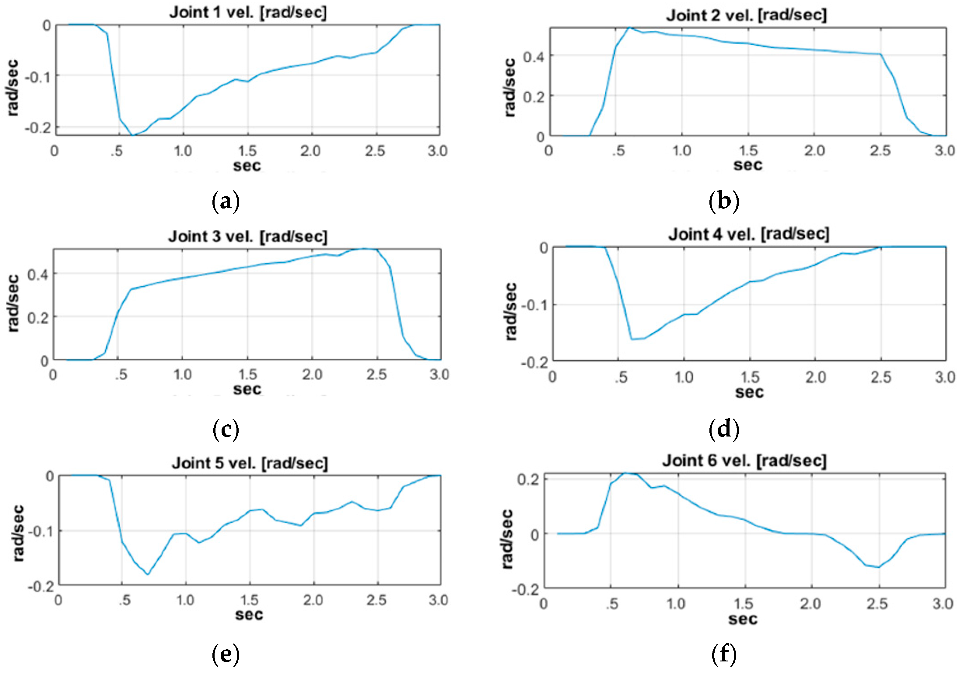
where , , , , and are joint velocities. Figure 7 shows the velocity ramp for each joint during the validation.
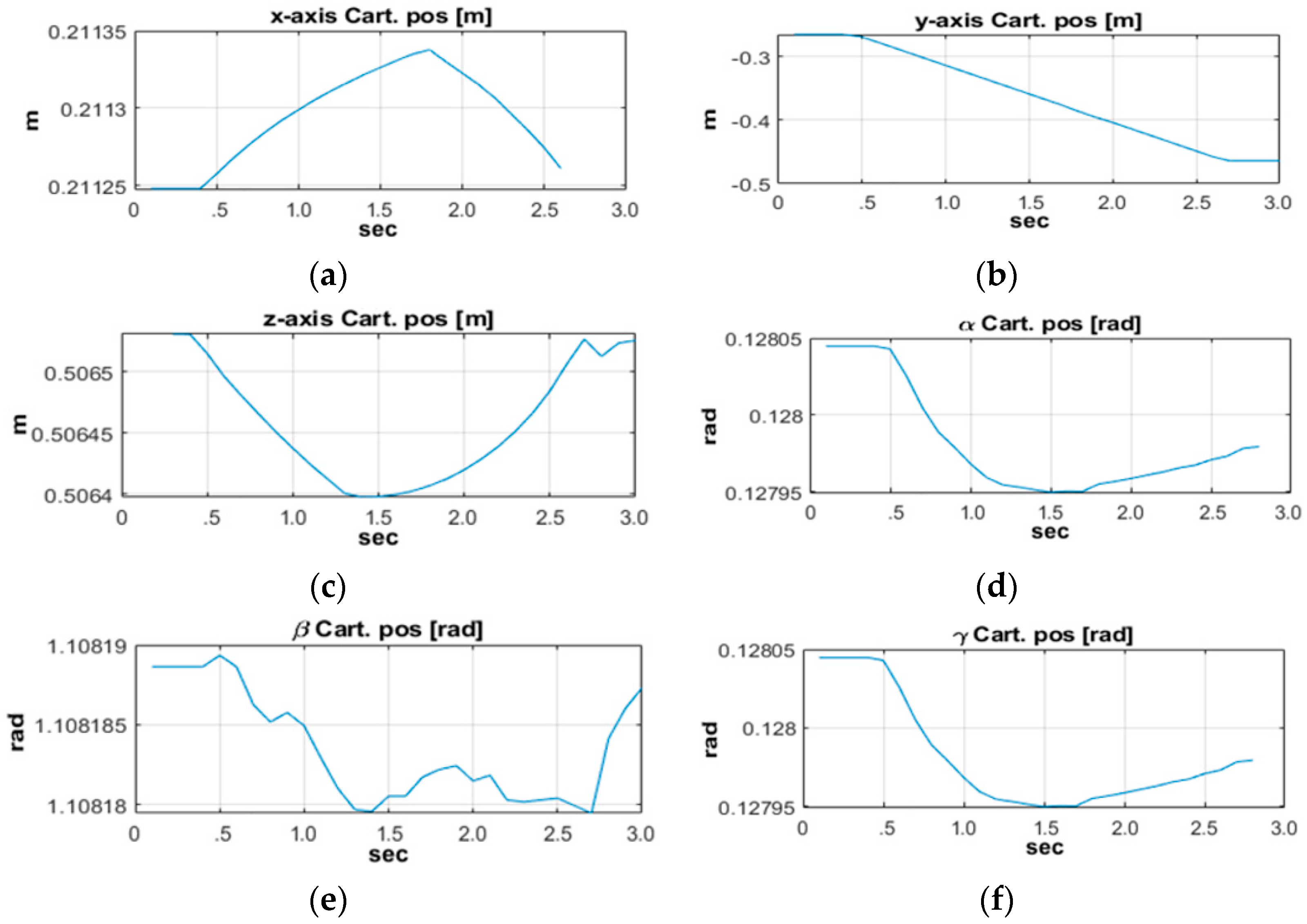
The positions along the axes and the orientations around them for the end-effector in the Cartesian coordinate system are shown in Figure 8.
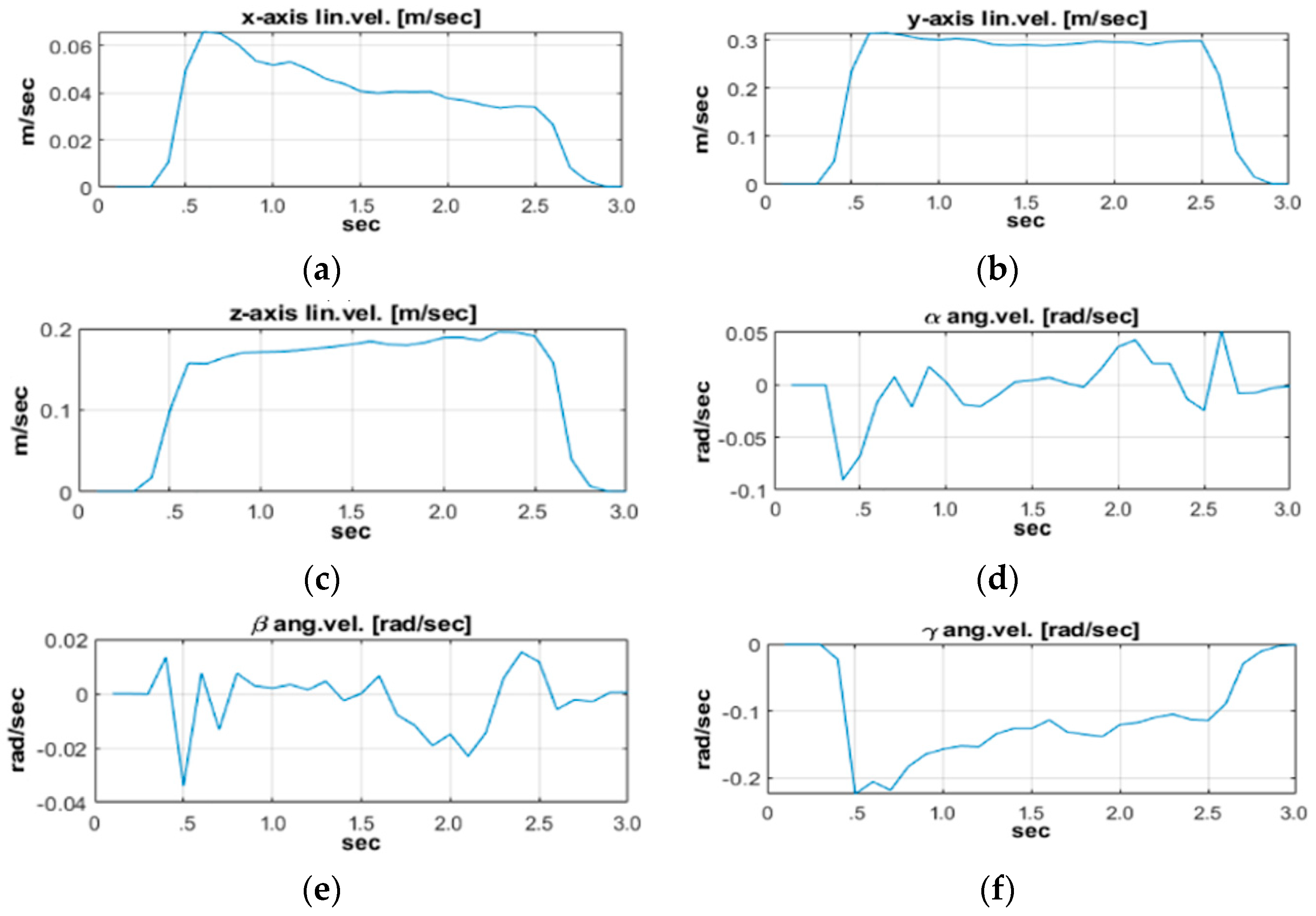
The values of the vector elements that represent the linear and angular velocities during the experiment are shown in Figure 9. It visualizes the results of applying formula (98). The velocities of the joints are applied to the earlier proposed algorithm. It calculates the vector that is given in . The values inside the vector provide a stable position for the end-effector in the 3D space, despite the movable base.
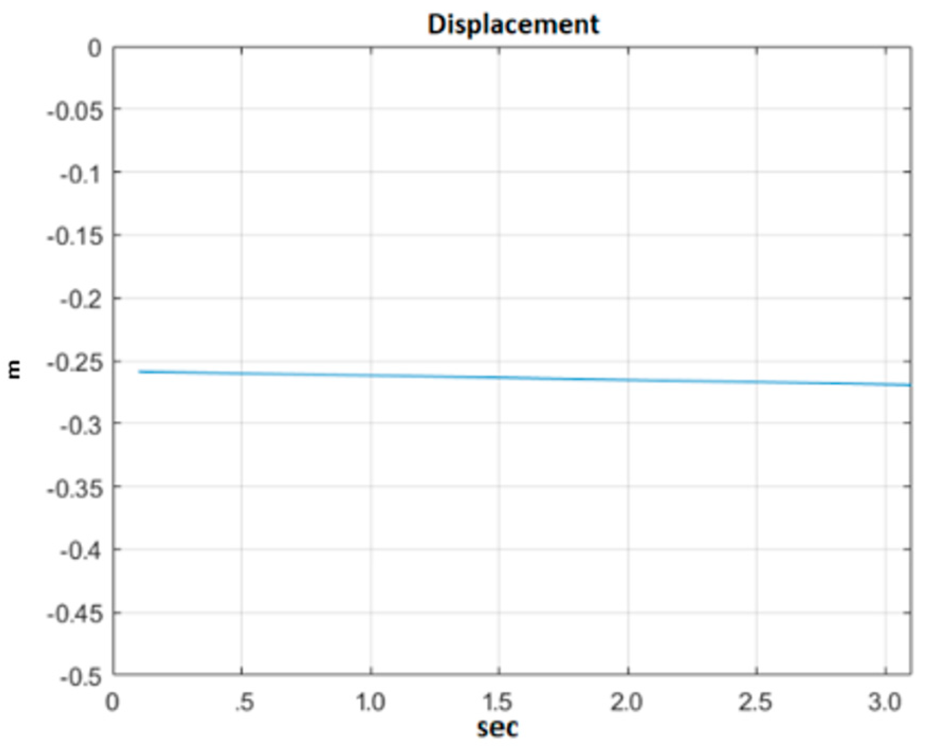
The displacement between the positions of the end-effector of the Kinova Jaco Gen 2 manipulator and the KUKA youBot mobile platform during the experiment is presented in Figure 10.
According to the proposed approach, we calculated the manipulator’s velocity along the axes of its base frame to keep its end-effector ’s position constant during the movement of the base. The base is attached to the mobile platform KUKA youBot. To validate the proposed approach, we visualized manipulator’s position along its y axis during the movement of the mobile robot. The manipulator’s home position along y axis is around −0.25 m. The horizontality of the line shows that the velocities of the manipulator and mobile robot are approximately the same, slightly observable slope may be caused by not perfect environment conditions like the slippage of the mobile platform’s wheels.
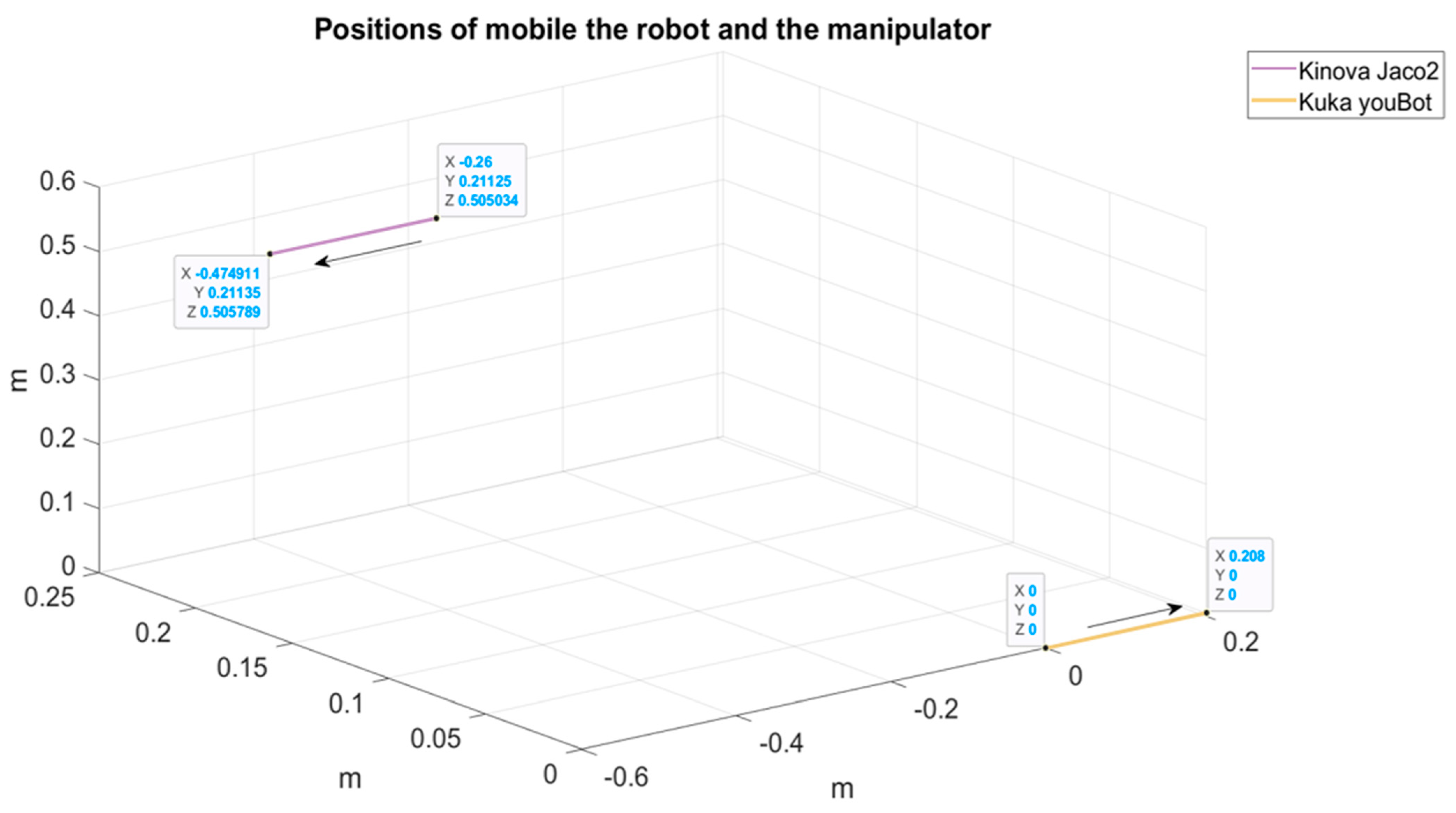
Figure 11 shows the positions of the mobile platform and the manipulator gripper during the experiment. Additionally, the starting and the final positions of their movements are visible.
4. Conclusions
We have proposed an affordable open-source mobile manipulator composed of the KUKA youBot mobile platform and a Kinova Jaco manipulator, and we have developed corresponding kinematic problems. The later have been verified by running experiments with the designed laboratory prototype. The proposed open-source character of the mobile manipulator and the initial software provided by the ROS community can help robot researchers to concentrate directly on their research topics. The latter can more easily complete challenging research and development tasks, which will accelerate the technology’s transfer and application.
Author Contributions
Conceptualization, A.V.T. and S.A.-S.; methodology, V.P. and S.A.-S.; software, V.P. and T.S.; validation, T.S. and V.P.; formal analysis, V.P.; investigation, S.A.-S.; resources, A.V.T. and S.A.-S.; data curation, T.S.; writing—original draft preparation, V.P.; writing—review and editing, A.V.T., T.S. and S.A.-S.; visualization, V.P. and T.S.; supervision, A.V.T.; project administration, S.A.-S.; funding acquisition, S.A.-S. and V.P. All authors have read and agreed to the published version of the manuscript.
Funding
The European Regional Development Fund within the Operational Programme “Bulgarian national recovery and resilience plan”, via the procedure for the direct provision of grants ”Establishing of a network of research higher education institutions in Bulgaria”, and under Project BG-RRP-2.004-0005, “Improving the research capacity anD quality to achieve intErnAtional recognition and reSilience of TU-Sofia (IDEAS)”.
Data Availability Statement
Data are available upon request.
Conflicts of Interest
The authors declare no conflicts of interest. The funders had no role in the design of the study; the collection, analyses, or interpretation of data; the writing of the manuscript; or the decision to publish the results.
References
- ISO/TS 15066:2016; Robots and Robotic Devices—Collaborative Robots. International Organization for Standardization: Geneva, Switzerland, 2016. Available online: https://www.iso.org/standard/62996.html (accessed on 16 January 2024).
- ISO 10218-1:2011; Robots and Robotic Devices—Safety Requirements for Industrial Robots—Part 1: Robots. International Organization for Standardization: Geneva, Switzerland, 2011. Available online: https://www.iso.org/standard/51330.html (accessed on 16 January 2024).
- ISO 10218-2:2011; Robots and Robotic Devices—Safety Requirements for Industrial Robots—Part 2: Robot Systems and Integration. International Organization for Standardization: Geneva, Switzerland, 2011. Available online: https://www.iso.org/standard/41571.html (accessed on 16 January 2024).
- Neto, P.; Pires, J.N.; Moreira, A.P. Accelerometer-based control of an industrial robotic arm. In Proceedings of the Robot and Human Interactive Communication RO-MAN 2009, Toyama, Japan, 27 September–2 October 2009. [Google Scholar] [CrossRef]
- Ben Abdallah, I.; Bouteraa, Y. Gesture Control of 3DOF Robotic Arm Teleoperated by Kinect Sensor. In Proceedings of the 19th International Conference on Sciences and Techniques of Automatic Control & Computer Engineering (STA), Sousse, Tunisia, 24–26 March 2019. [Google Scholar] [CrossRef]
- Ahmed, S.A.; Ramadan, M.M.; Fathy, E. Motion Control of Robot by Using Kinect Sensor. Res. J. Appl. Sci. Eng. Technol. 2014, 8, 1384–1388. [Google Scholar] [CrossRef]
- Waldherr, S.; Romero, R.; Thrun, S.A. Gesture Based Interface for Human-Robot Interaction. Auton. Robot. 2000, 9, 151–173. [Google Scholar] [CrossRef]
- Tchon, K.; Jakubiak, J.; Muszynski, R. Mobile manipulators with implicit aboard kinematics. In Proceedings of the 11th International Conference on Advanced Robotics ICAR 2003, Coimbra, Portugal, 30 June–3 July 2003. [Google Scholar] [CrossRef]
- Bischoff, R.; Huggenberger, U.; Prassler, E. KUKA youBot—A mobile manipulator for research and education. In Proceedings of the 2011 IEEE International Conference on Robotics and Automation, Shanghai, China, 9–13 May 2011. [Google Scholar] [CrossRef]
- Natarajan, S.; Kasperski, S.; Eich, M. An Autonomous Mobile Manipulator for Collecting Sample Containers. In Proceedings of the International Symposium on Artificial Intelligence, Robotics and Automation in Space, Montreal, Canada, 17-19 June 2014. [Google Scholar]
- Pepe, A.; Chiaravalli, D.; Melchiorri, C. A Hybrid Teleoperation Control Scheme for a Single-Arm Mobile Manipulator with Omnidirectional Wheels. In Proceedings of the 2016 IEEE/RSJ International Conference on Intelligent Robots and Systems (IROS), Daejeon, Republic of Korea, 9–14 October 2016. [Google Scholar] [CrossRef]
- Adiwahono, A.H.; Chua, Y.; Tee, K.P.; Liu, B. Automated door opening scheme for non-holonomic mobile manipulator. In Proceedings of the 2013 13th International Conference on Control, Automation and Systems (ICCAS 2013), Gwangju, Republic of Korea, 20–23 October 2013. [Google Scholar] [CrossRef]
- Zimmermann, S.; Poranne, R.; Coros, S. Go Fetch!—Dynamic Grasps using Boston Dynamics Spot with External Robotic Arm. In Proceedings of the 2021 IEEE International Conference on Robotics and Automation (ICRA), Xi’an, China, 30 May–5 June 2021. [Google Scholar] [CrossRef]
- Yamamoto, Y.; Yun, X. Coordinating locomotion and manipulation of a mobile manipulator. IEEE Trans. Autom. Contr. 1994, 39, 1326–1332. [Google Scholar] [CrossRef]
- Seraji, H. A unified approach to motion control of mobile manipulators. Int. J. Rob. Res. 1998, 17, 107–118. [Google Scholar] [CrossRef]
- Khatib, O.; Yokoi, K.; Chang, K.; Casai, A. Robots in human environments: Basic autonomous capabilities. Int. J. Rob. Res. 1999, 18, 684–696. [Google Scholar] [CrossRef]
- Yamamoto, Y.; Yun, X. Unified analysis of mobility and manipulability of mobile manipulators. In Proceedings of the Proceedings 1999 IEEE International Conference on Robotics and Automation (Cat. No.99CH36288C), Detroit, MI, USA, 10–15 May 1999; pp. 1200–1206. [Google Scholar] [CrossRef]
- Tchon, K.; Jakubiak, J.; Muszynski, R. Kinematics of mobile manipulators: A control theoretic perspective. Arch. Control Sci. 2001, 11, 79–105. [Google Scholar]
- Sharma, S.; Kraetzschmar, G.K.; Scheurer, C.; Bischoff, R. Unified Closed Form Inverse Kinematics for the KUKA youBot. In Proceedings of the ROBOTIK 2012, 7th German Conference on Robotics, Munich, Germany, 21–22 May 2012; ISBN 978-3-8007-3418-4. [Google Scholar]
- Liu, Y.; Li, H.; Ding, L.; Liu, L.; Liu, T.; Wang, J.; Gao, H. An Omnidirectional Mobile Operating Robot Based on Mecanum Wheel. In Proceedings of the 2017 2nd International Conference on Advanced Robotics and Mechatronics (ICARM), Hefei and Tai’an, China, 27–31 August 2017. [Google Scholar] [CrossRef]
- Li, X.; Luo, L.Z.; Zhao, H.; Ge, D.S.; Ding, H. Inverse Kinematics Solution Based on Redundancy Modeling and Desired Behaviors Optimization for Dual Mobile Manipulators. J. Intell. Robot. Syst. 2023, 108, 37. [Google Scholar] [CrossRef]
- Zhang, X.F.; Li, G.F.; Xiao, F.; Jiang, D.; Tao, B.; Kong, J.Y.; Jiang, G.Z.; Liu, Y. An inverse kinematics framework of mobile manipulator based on unique domain constraint. Mech. Mach. Theory 2023, 183, 105273. [Google Scholar] [CrossRef]
- Colucci, G.; Botta, A.; Tagliavini, L.; Cavallone, P.; Baglieri, L.; Quaglia, G. Kinematic Modeling and Motion Planning of the Mobile Manipulator Agri.Q for Precision Agriculture. Machines 2022, 5, 321. [Google Scholar] [CrossRef]
- Huang, Y.; Li, D.L.; Dong, K.J.; Zhang, W.C.; Gao, X.M. Inverse Kinematics Analysis and Mechatronics Design of Mobile Parallel Manipulator for Assisted Assembly. In Proceedings of the 2022 IEEE International Conference on Mechatronics and Automation (IEEE ICMA 2022), Guilin, China, 7–10 August 2022. [Google Scholar] [CrossRef]
- Siegwart, R.; Nourbakhsh, I.R.; Scaramuzza, D. Introduction to Autonomous Mobile Robots; The MIT Press: Cambridge, MA, USA, 2011. [Google Scholar]
- Ahmed, S.A.; Shakev, N.G.; Topalov, A.V.; Popov, V.L. Model-Free Detection and Following of Moving Objects by an Omnidirectional Mobile Robot using 2D Range Data. IFAC-PapersOnLine 2018, 51, 226–231. [Google Scholar] [CrossRef]
- User Guide KINOVA® GEN2 Ultra Lightweight Robot. Available online: https://artifactory.kinovaapps.com/ui/api/v1/download?repoKey=generic-documentation-public&path=Documentation%252FGen2%252FTechnical%2520documentation%252FUser%2520Guide%252FUG-009_KINOVA_Gen2_Ultra_lightweight_robot_User_guide_EN_R03.pdf (accessed on 21 October 2023).
- Craig, J.J. Introduction to Robotics: Mechanics and Control, 4th ed.; Pearson Prentice Hall: London, UK, 2017. [Google Scholar]
- Lewis, W.L.; Dawson, D.M.; Abdallag, C.T. Robot Manipulator Control Theory and Practice, 2nd ed.; Publisher Marcel Dekker, Inc.: New York, NY, USA, 2004. [Google Scholar]
Figure 1.
Mobile manipulator and velocities.

Figure 2.
Geometric dimensions (in [mm]) of the mobile platform KUKA youBot.

Figure 3.
A sketch with the necessary notations to calculate the forward kinematics of the mobile platform: (a) wheel parameters and (b) wheels and the corresponding speeds.
Figure 3.
A sketch with the necessary notations to calculate the forward kinematics of the mobile platform: (a) wheel parameters and (b) wheels and the corresponding speeds.

Figure 4.
Notations (a) and dimensions (b) of Jaco Gen 2 manipulator.

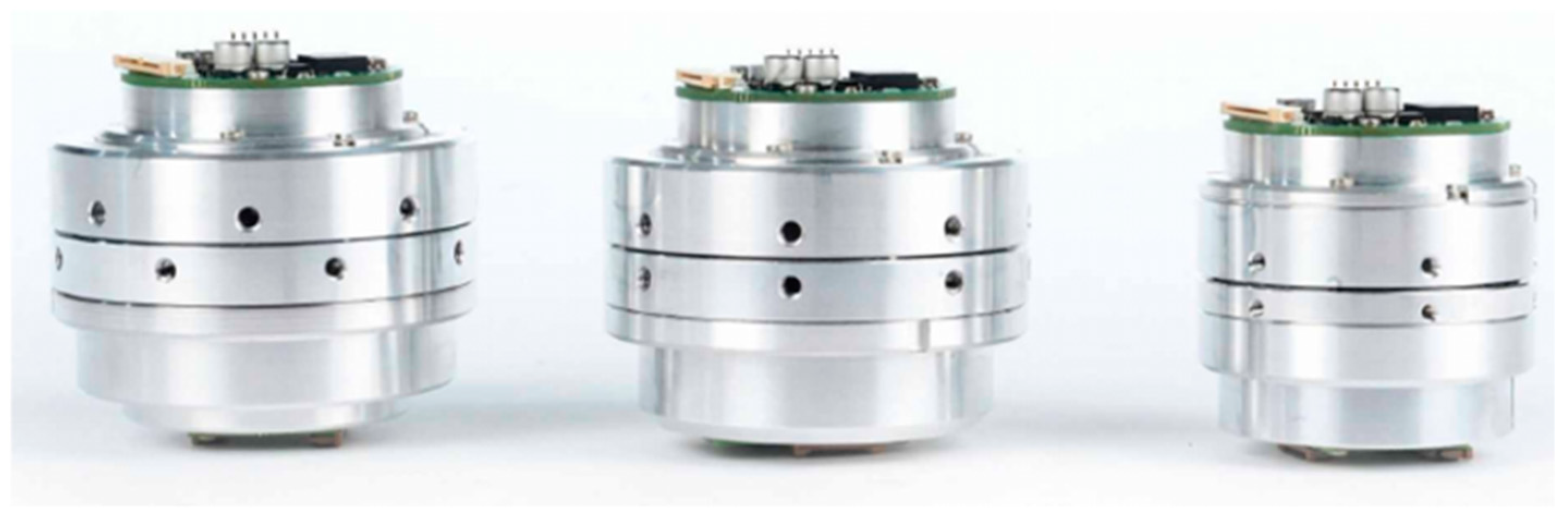
Figure 5.
Kinova’s actuators: K-75+, K-75 and K-58.

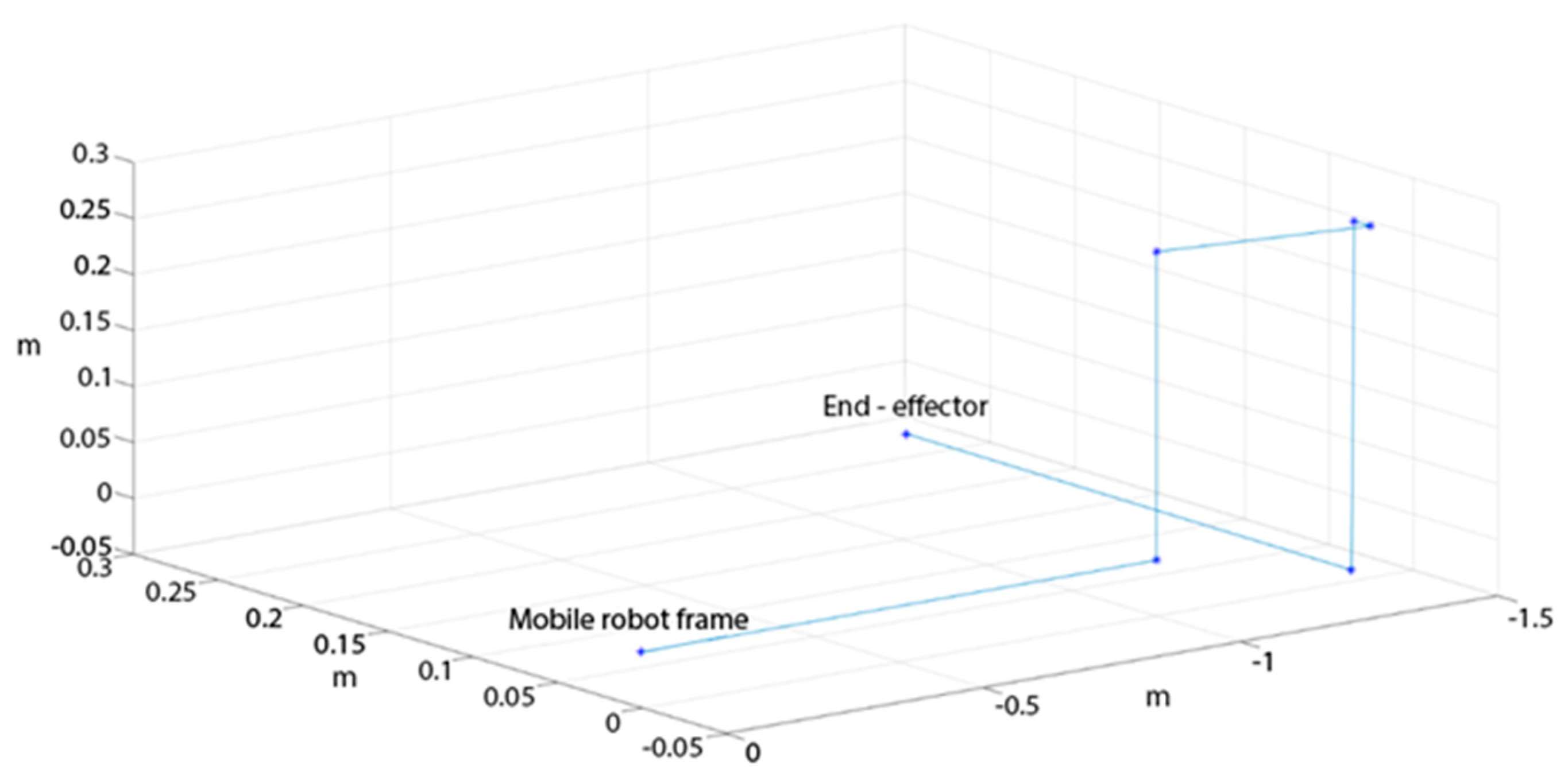
Figure 6.
Position of the end-effector according to the mobile platform frame. The manipulator is placed in home position.
Figure 6.
Position of the end-effector according to the mobile platform frame. The manipulator is placed in home position.

Figure 7.
Joint velocities: (a) velocity of the first joint; (b) velocity of the second joint; (c) velocity of the third joint; (d) velocity of the fourth joint; (e) velocity of the fifth joint; (f) velocity of the sixth joint.
Figure 7.
Joint velocities: (a) velocity of the first joint; (b) velocity of the second joint; (c) velocity of the third joint; (d) velocity of the fourth joint; (e) velocity of the fifth joint; (f) velocity of the sixth joint.

Figure 8.
Measured positions and orientations of the end-effector. There are 3 positions and 3 orientations according to the manipulator’s base (Cartesian) coordinate system: (a) position along the axis; (b) position along the axis; (c) position along the axis; (d) orientation around the axis—; (e) orientation around the axis—; (f) orientation around the axis—.

Figure 9.
Calculated velocities according to the manipulator’s base coordinate system, along each axis and around each axis. These velocities applied to the base provide constant position of the end-effector during its movement according to the adjusted joint velocities vector : (a) velocity along the axis; (b) velocity along the axis; (c) velocity along the axis; (d) velocity around the axis; (e) velocity around the axis; (f) velocity around the axis.

Figure 10.
Displacement between the position of the movable base coordinate system and the position of the end-effector.
Figure 10.
Displacement between the position of the movable base coordinate system and the position of the end-effector.

Figure 11.
The positions of the mobile platform and manipulator gripper during the experiment.


Table 1.
Kinematic parameters of the mobile platform.
| β [deg] | |||||
|---|---|---|---|---|---|
| Wheel (1) | 32.5 | 57.5 | −45 | 0.279 | 0.05 |
| Wheel (2) | 147.5 | −57.5 | 45 | 0.279 | 0.05 |
| Wheel (3) | −147.5 | −122.5 | −45 | 0.279 | 0.05 |
| Wheel (4) | −32.5 | 122.5 | 45 | 0.279 | 0.05 |
Table 2.
Structural elements of the homogeneous transformations [27].
Table 2.
Structural elements of the homogeneous transformations [27].
| Parameters | Descriptions | Length (m) |
|---|---|---|
| Base to shoulder | 0.2755 | |
| Upper Length (shoulder to elbow) | 0.41 | |
| Forearm length (elbow to wrist) | 0.2073 | |
| First wrist length | 0.1038 | |
| Second wrist length | 0.1038 | |
| Wrist to center of the hand | 0.16 | |
| Joint 3–4 lateral offset | 0.0133 |
Table 3.
Physical characteristics of the manipulator Jaco Gen2 [27].
Table 3.
Physical characteristics of the manipulator Jaco Gen2 [27].
| Characteristics | Values |
|---|---|
| Total weight | 4.4 kg |
| Reach | 98.4 cm |
| Maximum payload | 2.6 kg (mid-range)/2.2 kg (full-range) |
| Materials | carbon fiber/aluminum |
| Maximum linear arm speed | 20 cm/sec |
| Power supply voltage | 18–29 VDC |
| Average power | 25 W (15 W standby) |
| Peak power | 100 W |
| Communication protocol | RS485 |
| Communication cables | 20 pins flat flex cable |
| Water resistance | IPX2 |
| Operating temperature | −10 to 40 |
Table 4.
Kinova Jaco Gen 2’s actuator specifications.
| Title | |||
|---|---|---|---|
| Nominal torque (Nm) | 12 | 9.2 | 3.6 |
| Peak torque (Nm) | 30.5 | 18 | 6.8 |
| No load speed (rpm) | 12.2 | 9.8 | 20.3 |
| Nominal speed (rpm) | 9.4 | 7 | 15 |
| Weight (g) | 570 | 587 | 357 |
| Reduction ratio | 136 | 160 | 110 |
| Angular ranges, software limited (turns) | ±27.7 | ||
| Communication protocol | RS485 | ||
Table 5.
Table formed using Denavit–Hartenberg parameters, classical approach [27].
Table 5.
Table formed using Denavit–Hartenberg parameters, classical approach [27].
| 1 | 0 | |||
| 2 | 0 | |||
| 3 | 0 | |||
| 4 | 0 | |||
| 5 | 0 | 0 | ||
| 6 | 0 |
Table 6.
Table formed by Denavit–Hartenberg parameters, using a modified approach.
| 1 | 0 | 0 | ||
| 2 | 0 | 0 | ||
| 3 | ||||
| 4 | 0 | |||
| 5 | 0 | 0 | ||
| 6 | 0 |
Disclaimer/Publisher’s Note: The statements, opinions and data contained in all publications are solely those of the individual author(s) and contributor(s) and not of MDPI and/or the editor(s). MDPI and/or the editor(s) disclaim responsibility for any injury to people or property resulting from any ideas, methods, instructions or products referred to in the content. |
© 2024 by the authors. Licensee MDPI, Basel, Switzerland. This article is an open access article distributed under the terms and conditions of the Creative Commons Attribution (CC BY) license (https://creativecommons.org/licenses/by/4.0/).
Share and Cite
MDPI and ACS Style
Popov, V.; Topalov, A.V.; Stoyanov, T.; Ahmed-Shieva, S. Kinematic Modeling with Experimental Validation of a KUKA®–Kinova® Holonomic Mobile Manipulator. Electronics 2024, 13, 1534. https://doi.org/10.3390/electronics13081534
AMA Style
Popov V, Topalov AV, Stoyanov T, Ahmed-Shieva S. Kinematic Modeling with Experimental Validation of a KUKA®–Kinova® Holonomic Mobile Manipulator. Electronics. 2024; 13(8):1534. https://doi.org/10.3390/electronics13081534
Chicago/Turabian StylePopov, Vasil, Andon V. Topalov, Tihomir Stoyanov, and Sevil Ahmed-Shieva. 2024. "Kinematic Modeling with Experimental Validation of a KUKA®–Kinova® Holonomic Mobile Manipulator" Electronics 13, no. 8: 1534. https://doi.org/10.3390/electronics13081534
Note that from the first issue of 2016, this journal uses article numbers instead of page numbers. See further details here.