

The Emptying of a Perforated Bottle: Influence of Perforation Size on Emptying Time and the Physical Nature of the Process

Department of Mechanical Engineering, California Polytechnic State University, San Luis Obispo, CA 93407, USA
*
Author to whom correspondence should be addressed.
Fluids 2023, 8(8), 225; https://doi.org/10.3390/fluids8080225
Submission received: 9 July 2023
/
Revised: 17 July 2023
/
Accepted: 25 July 2023
/
Published: 4 August 2023
(This article belongs to the Special Issue Advances in Multiphase Flow Science and Technology, 2nd Edition)
Abstract
:An inverted bottle empties in a time through a process called “glugging”, whereby gas and liquid compete at the neck (of diameter ). In contrast, an open-top container empties in a much shorter time through “jetting” due to the lack of gas–liquid competition. Experiments and theory demonstrate that, by introducing a perforation (diameter ), a bottle empties through glugging, jetting, or a combination of the two. For a certain range of , the perforation increases the emptying time, and a particular value of is associated with a maximum emptying time . We show that the transition from jetting to glugging is initiated by the jet velocity reaching a low threshold, thereby allowing a slug of air entry into the neck that stops jetting and starts the glugging. Once initiated, the glugging proceeds as though there is no perforation. Experimental results covered a range of Eötvös numbers from Eo∼ 20–200 (equivalent to a range of 4–15, where is the capillary length). The phenomenon of bottle emptying with a perforation adds to the body of bottle literature, which has already considered the influence of shape, inclination, liquid properties, etc.
1. Introduction
1.1. Motivation: An Interesting and Novel Observation
A bottle (i.e., a single-outlet vessel) that is filled with liquid, inverted, and emptied will exhibit the familiar “glugging” phenomenon in which air and water compete for entry and exit through the neck. The motivation for the experimental and theoretical investigation presented in this work stems from an interesting set of original observations, shared with the authors [1], that were made during the course of such bottle emptying experiments. In those experiments, store-bought plastic water bottles were perforated, at a location opposite the neck, with various sizes of twist drills and needles. These bottles were then filled with water, corked, inverted, and emptied. The time to empty the bottle, , was recorded for each perforation diameter, . The quantitative results of those experiments are provided in Figure 1a and present an interesting picture.
Figure 1a shows that the maximum emptying time was not associated with glugging throughout the entire emptying event (which corresponds to = 0), which we denoted with time . In addition, the emptying time did not monotonically decrease with the increasing perforation diameter. Instead, there appeared to be a range of perforation diameters for which the emptying time exceeded , and there appeared to be a value of that corresponded to a maximum emptying time . For this particular bottle, the maximum emptying time was ∼25% larger than the . The original experiments that led to the data in Figure 1a were rather crude. The bottles were held in their inverted position by hand and timed by hand. Only eight different perforation sizes were used.
The phenomenon was replicated in a more systematic investigation. For this second set of experiments, a team of undergraduate student researchers were employed to again fill, invert, empty, and time bottles by hand. Improvements over the original experiments include: the use of several researchers (four) to reduce artifacts in the experiment data and observations that could be the result of a single investigator’s unintended bias; using thicker-walled plastic bottles (increased rigidity); and testing with a larger number of values near . Each researcher used the same fifteen bottles (one control bottle, , and fourteen different sizes). The results of these experiments are shown in Figure 1b. Again, the maximum emptying time was associated with a particular size perforation. What was striking was that the maximum emptying time was nearly 100% larger than the for this case.
Figure 1.
Data from simple bottle-emptying experiments (i.e., hand-held inverted bottles) yielded the interesting observation that a maximum emptying time occurred for a particular value of perforation diameter . (a) The original experiments that initiated the study (performed by Researcher 1). (b) A more complete set of experiments, performed by four new student researchers (listed as Researchers 2–5) and using a different bottle than (a), which confirmed the original observations. Error bars represent the standard deviation of measurements for each condition.

During these confirmation experiments, the researchers were also asked to make qualitative observations about how the bottles emptied by classifying the emptying as occurring by only glugging (air–water competition through the neck), only jetting (only water exiting the neck), or a combination of jetting and glugging J-G. It was observed that bottles emptied by these three mechanisms and that, if a bottle transitioned between the two, it always commenced with jetting, followed by glugging at some time and height during the emptying process. By combining the quantitative results for and the qualitative observations, a trend emerged, shown in Figure 1b, that the maximum emptying time was associated with a particular combination of emptying through jetting and glugging. Additionally, the overlap of data from the four researchers confirmed the repeatability of the observed behavior, both in terms of the magnitude of the emptying times and the value of leading to the .
Figure 2.
The characteristics of the emptying process, which translates directly into the value of the emptying time , of an inverted bottle are highly dependent on the size of a perforation introduced on the top of the bottle. Sequences (a–c) show images taken at equal intervals of time from 10–90% of the total emptying time. (a) A bottle with no perforation () empties through a “glugging” process and, in this case, takes ∼8 s. Note that the level in the bottle drops nearly linearly with time. (b) A bottle that has had the top removed, thus creating an open-top vessel () drains via a“jetting”process where no air enters into the neck. This particular draining event is rapid and takes ∼1 s. The undisturbed air–water interface within the bottle is seen to descend non-linearly. (c) If a small perforation is introduced on the top of the bottle (), draining initially proceeds through jetting but transitions at some time (and corresponding height) to glugging. This occurs between the sixth and seventh frames of the sequence. For this case, the total draining process takes ∼13 s, with glugging accounting for 38% of . The images in (a–c) are from experiments performed to highlight the various emptying regimes. A clear plastic bottle with a height H = 174 mm, = 21.6 mm, D = 62.5 mm, and internal volume of V = 490 mL was used. The perforation introduced in the bottle for case (c) was made using a #58 drill ( = 1.07 mm, = 0.050). Images were extracted from movies recorded using a Phantom v310 high-speed camera. Plots to the right of each image sequence show a measurement of the liquid jet diameter, , measured at a distance of from the outlet, during the emptying process (solid lines). Significant fluctuations in jet diameter occurred during glugging, but when jetting, the jet diameter smoothly decreases with time (and reduced flow rate). The plots show that when jetting transitions to glugging, the glugging is essentially indistinguishable from the glugging-only case. The dimensionless level of the air–water interface, , is also tracked (dashed lines).

To better illustrate the phenomenon, a few representative experiments were performed, using clear bottles and a high speed camera, in order to capture the various emptying processes. Sequences of images from emptying conditions that produce only glugging, only jetting, and a jetting-to-glugging transition are presented in Figure 2. These are provided only for the purpose of visually illustrating the phenomena described and do not constitute the formal results. In addition to photographs that illustrate the emptying processes, the diameter of the jet at a distance of one neck diameter from the outlet, as well as the fraction of the bottle height filled with water (i.e., tracking the air–water interface), was measured from the movie frames to further highlight the transition and distinct differences between glugging and jetting.
1.2. Key Questions
There are several key questions about the emptying of perforated bottles that emerge from the simple sets of experiments presented: (1) Under what conditions does a perforated bottle achieve its maximum emptying time? It is obvious from the results of Figure 1 that, for any particular bottle, there exists a value of that yields a . So for an individual bottle, at what ratio of does the occur? (2) What other variables related to the bottle shape and size have an impact on the conditions for the maximum emptying time? It can already be suggested from the differences between the results in Figure 1 that the neck diameter may play a role. However, is there a universal ratio of that yields a maximum emptying time? (3) Qualitative observations suggest that the maximum emptying time results from some combination of jetting and glugging. What fraction of time consumed by either jetting or glugging resulted in the ? (4) What prompts the transition from jetting to glugging? This transition appears to blend together two types of emptying processes that have already been studied. The mechanism that causes this transition is the link that can help explain the phenomenon of emptying with a perforation. What follows is a presentation of the results of the experiments and theoretical modeling, which attempt to answer the key questions.
2. Literature Review
Preliminary experiments have demonstrated the novel finding that a perforated bottle can empty by glugging, jetting, or a combination of the two regimes—meaning that the bottle will empty first by jetting and then transition to glugging at some point during the process (cf. Figure 2c). Thus, a basic review of the literature is in order to understand both the experimental results and the theoretical modeling presented later, in addition to providing a survey of the current state of the art for the field.
2.1. Glugging
The field of two-phase flow, including the study of the motion of bubbles in tubes (e.g., the work of Davies and Taylor [2] among others), has a long and rich history, as well as an extensive literature. A small portion of that literature has been occupied by investigations of the emptying of single-outlet vessels—either in the form of commercially available bottles or experimental apparatuses designed with controlled features and geometries (i.e., “ideal” bottles). The earliest published works in this area can be attributed to Whalley [3,4], who experimentally investigated the time to empty commercially available bottles. In recognizing that the competing flows of air and water at the bottle neck were similar to the processes of flooding and slugging in tubes, Whalley used his measurements to quantify and report flooding constants. He found that these constants, and, hence, the emptying time, could be influenced by the angle of bottle inclination, adjustments to the bottle neck length, and water temperature (an ∼10% decrease in emptying time with a 30 °C increase in water temperature). These findings were in addition to the basic discovered trends that the emptying time increases with decreasing neck diameter and increasing bottle volume. By using small commercially available bottles (less than a few liters in volume), Whalley was able to measure the overall emptying time, but not the details of the height of the air–water interface within the bottles. The influence of bottle inclination was investigated more recently by Rohilla and Das [5].
Following the works of Whalley, Schmidt and Kubie [6] used ideal bottles fabricated out of constant-diameter tubes having outlets formed by holes in thick flat plates (the outlets are somewhere between a sharp-edged orifice and an elongated bottle neck). Those authors tracked the air–water interface during the course of emptying, using a sight tube on the sides of their bottles, and reported that the magnitude of the interface velocity remained nearly constant during emptying but changed with the shape of the outlet. Kubie and his collaborators used these types of ideal bottles to further investigate the pressure oscillations during emptying [7] and the effect of outlet orifice inclination on the emptying process [8].
Many of the same trends observed by previous bottle emptying investigators were reported again by Clanet and Searby [9], who published the results of a detailed set of experiments and theory on the “glug-glug” of ideal bottles—hence our use of the term “glugging” to describe the regime shown in Figure 2a. For example, Clanet and Searby reported a near constant velocity of the air–water interface within the bottle while emptying. These authors not only studied the overall bottle emptying time (which they termed the ‘long time-scale’), but the nature of the oscillations as well. The transparent tubes used by Clanet and Searby allowed for internal visualization during emptying. The outlets of their bottles were formed by holes in thin plates (creating sharp-edged orifices). This type of outlet geometry was in contrast to those of Schmidt and Kubie [6], and both were distinct from the outlets used in the experiments reported in the present work (cf. Section 3).
A result from the Clanet and Searby study, utilized later, is their model that predicts the overall emptying time of a bottle. Their conclusion, which was validated by experiments, is that the time scale is related to the overall height of the bottle H, the bottle diameter D, and the neck diameter through the following equation:
This model, which we will refer to as the Clanet model, was developed by balancing over a unit time the incoming volume of air through the neck with the outflow of water (related to the velocity of the air–water interface within the bottle), and it assumes that the two fluids are incompressible. In other words, , where U is the velocity of the air–water interface within the bottle of diameter D, is the upward velocity of the air through the neck of diameter , and is a fraction that describes the occupancy of air in the neck over the unit time. Clanet and Searby, guided by the Davies and Taylor [2] analysis of long bubbles rising in tubes under conditions for which viscous and surface tension effects are negligible, chose to model . The variable is a dimensionless number, with limits of 0 and 1, which is related to the size of the slug that enters the bottle through the neck over the unit time. A value of was used by Clanet and Searby, which provided agreement with their data.
Experimental observations show that the velocity U within a bottle is a weak function of the air–liquid interface height h (which varies over time between the overall bottle height H and 0). Therefore, Equation (1) can be rearranged to show this relationship:
which indicates that U will increase with increasing and that . Since it has been reported that U is nearly constant throughout emptying via the glugging process, it is no surprise then that .
It is worth noting two more recent studies that were published during the course of our experiments, which are related to the phenomenon described here. The first new study by Kumar et al. [10] involved the draining of constant-diameter, vertically oriented tubes whose ends were initially capped but then sequentially pierced to allow the entry of air into the top of the tube. This is equivalent to a bottle for which . They found that these piercings, similar to our work with bottles, influenced both the nature of the flow and the overall emptying time. A key difference between that study and the work presented here is that the tubes did not empty via a glugging process, but rather drained by the introduction of a long Taylor finger (when not pierced) or through full bore draining when . However, they did find that, for a range of piercing sizes such that , a coupling of the mechanisms could be achieved. With respect to even more recent than the work of Kumar et al., Liang et al. [11] reported on the emptying of tanks with cylindrical and elliptical outlets and found that venting the tank could produce different trends in . It is unclear from their study whether they observed any conditions for which the emptying process transitioned from jetting to glugging. Instead, it appears that they only noticed the difference between trends for the glugging-only case and the jetting-only case. This was likely due to the values of , which we estimated to be ∼. Liang et al. did not identify that “ventilation”, as they termed it, could lead to an increase in the emptying time beyond that achieved by glugging.
2.2. Jetting
The term “jetting” refers to the scenario in the emptying of a perforated inverted bottle (or the extreme case of an open top bottle), where a sufficient quantity of air is allowed through the perforation such that only liquid exits the neck (cf. Figure 2b). This is in stark contrast to “glugging”. Note that “jetting” implies that the velocity (and flow rate) of the jet of liquid exiting the bottle neck is sufficient to the point that no “dripping” occurs during the emptying process. In other words, the breakup length of the jets are observed to be very long in comparison to the jet diameters. The transition from jetting to dripping, which is caused by a reduction in the imposed flow rate, has been studied, see, e.g., Clanet and Lasheras [12], but not for the case of bottles where the flow rate is not a controlled parameter. The conditions of our experiments (i.e., large neck sizes—well above the capillary length—and sufficiently large flow rates) were such that dripping played no role.
Because of the single-phase flow nature through both the perforation (gas) and neck (liquid), the jetting scenario can be treated using a traditional energy method (e.g., treating the flow through either the perforation or the neck as a pipe flow problem). Since this technique is ubiquitous, a review is not given here. Instead, the necessary equations are introduced in Section 4, but note that the velocity of liquid through the neck is not only dependent on the height of the liquid in the bottle, but also on the pressure above the air–water interface. This means that jetting is characterized by a non-linear trend of .
2.3. Jetting to Glugging and Bubble Rising
The transition from jetting-to-glugging behavior represents a change in flow regimes from single- to two-phase flow through the neck of a perforated inverted bottle. In addition, as glugging was already related to the phenomenon of bubble rising in tubes, and this must be related to the transition behavior, it makes sense to elaborate further on the subject. The early work of Davies and Taylor [2] examined the motion of a single air bubble rising through a vertical tube filled with liquid. In particular, the increasing of the velocity of large bubbles—those for which viscous and surface tension effects can be neglected—was under investigation. Davies and Taylor developed an experimentally validated relation for bubble rise velocity, , based on the tube diameter (we used the neck diameter as the tube diameter in the relations to follow) and gravity g. When reported as a dimensionless ratio, their findings follow,
where the dimensionless ratio is also used to define the bubble velocity coefficient k. The value shown in Equation (3) can be considered a limiting case corresponding to large bubbles, whereas, for single bubbles rising in smaller diameter tubes, k has been found to be less than this limiting condition. For example, Davies and Taylor found that for , , but for , . Other investigators, e.g., Dumitrescu [13] and White and Beardmore [14], reported similar values of k for large bubbles: and , respectively. Wallis [15] has referred to the value obtained by White and Beardmore as the preferred value of k.
When the bubble size decreases, i.e., tube diameter decreases, viscous and surface tension effects become more pronounced and lead to a reduction in the bubble rise velocity (hence, a reduction in k). These effects are captured in the following empirical relation provided by Wallis [15]:
where is the dimensionless inverse viscosity defined as , is the Eötvös number defined as , and m is a function of but is equal to 10 for the range of values of interest in this study, i.e., 1100–35,000. Within these dimensionless numbers, and are the liquid and gas densities, respectively (where ), is the liquid phase dynamic viscosity, and is the liquid–gas interfacial tension. The neck diameter was used frequently throughout this work, so we used to allow us to employ the convenient ratio of length scales when plotting the trend in k in the Results and Discussion section. The variable is the capillary length, which is . The conditions of our experiments corresponded to , which was a range of of (corresponding to 20–200). Another feature to point out from Equation (4) is that at the bubble velocity is predicted to be zero. This is the length scale below which a bubble cannot enter the tube due to surface tension effects. Such a value was reported by White and Beardmore [14] to be consistent with their experimentally observed limit of (provided as the value in the exponent of Equation (4)), but it was in contrast to the theoretical value predicted by the Rayleigh–Taylor instability of .
3. Materials and Methods
A series of experiments was implemented to investigate the emptying of a perforated bottle and answer key questions. Unfortunately, the COVID-19 pandemic coincided with this project. As with many institutions that were forced to curb research activities, our lab resources were restricted. Thus, we developed a simple experimental setup that could be used in an at-home setting and for which data could be collected manually (this is reminiscent of many of the early works on bottle emptying [3,6]). Since we relied on manual data collection, and one of the key questions was related to the fraction of bottle height and time occupied by either the jetting or glugging regimes, a very large bottle was constructed so that the height and time could be measured manually but with an attempt at minimizing measurement uncertainties. Note that all measurements were originally made using English units and have been converted to SI units for this paper. This explains some of the choices of dimensions (e.g., values of neck diameter ). Because of the limits on our equipment and facility resources, we had no method to control the temperature of the water used in our experiments, so we relied on ambient conditions. The collection of water temperature measurements using a Type K thermocouple from the experiments pointed to an average temperature of 26±1 °C (with a standard deviation of 2 °C). Even considering the extreme range of the measurements (approximately 20 °C to 30 °C), the fluid property variations were not significant enough to account for the phenomenon observed, and this was consistent with the temperature influence found by Whalley [3].
The bottle used for experiments was constructed from a commercially available (15 gallon, nominal volume) high density polyethylene (HDPE) plastic drum. A schematic diagram of the bottle is shown in Figure 3. The bottle had a diameter of and a height of approximately (with an estimated uncertainty of for both).
Figure 3.
(a) Schematic diagram of the large bottle with sight tube attached to measure . (b) A representative photograph of one of six 3D-printed plastic necks installed on the bottle.
Figure 3.
(a) Schematic diagram of the large bottle with sight tube attached to measure . (b) A representative photograph of one of six 3D-printed plastic necks installed on the bottle.

As supplied, the drum possessed two threaded ports on the top. The first port accommodated a diameter threaded drum plug. The plug had a rubber gasket to create a seal—which was necessary to prevent any unwanted perforation. This port was used to fill the drum with tap water prior to the start of each experiment. The second port accepted a smaller threaded plug. For each experiment that required a perforation, a hole was drilled into a PVC plug and inserted into this port. The diameter of the drill set the perforation diameter . The range of perforation sizes varied with neck diameter. Table 1 contains the range of sizes and the number of unique perforations tested for each neck. A majority of holes were drilled using either standard numbered drills, i.e., #1–#60 (5.79–1.02 mm diameters) or numbered micro-drills, i.e.,#61–#80 (0.99–0.34 mm diameters). For these perforation sizes, holes were drilled manually using a drill press or vertical mill, with a hand feed chuck for small drills (spindle speeds of ≈3 krpm). Measurements using a Micro-Vu Spectra optical comparator confirmed hole sizes within ≈ of nominal values (this represents the average over all numbered drill sizes). A few experiments required drills with nominal sizes of , , and . For these very small drill bits, a Haas Super Mini Mill 2 was utilized in order to achieve the 10 krpm speeds necessary. Holes made from these very small drills were then measured using a Micro-Vu Vertex coordinate measuring machine. For experiments requiring no holes, simulating a non-perforated bottle in order to measure , an un-perforated PVC plug was used. Teflon pipe tape was used on all plug threads to improve sealing.
The drum was modified into a bottle by incorporating an outlet and neck. The outlet was fabricated by first cutting a centrally located hole in the base of the drum that was approximately in diameter. Six holes were drilled circumferentially around this large hole to accept machine screws. Using these machine screws, 3D-printed plastic necks with a matching hole pattern could be secured to the base of the drum. A gasket between the 3D-printed neck and the drum base was installed. Each neck had a length of with one of six nominal neck diameters : , , , , , and . Measured neck diameters are reported in Table 1. Only one neck length and shape (i.e., square edge at neck) was tested in the present study.
Because the bottle was made of opaque plastic (HDPE), a means was necessary for viewing the height of the liquid level h inside the bottle. To accomplish this, a sight tube was constructed using clear plastic tubing (ID = 9.5 mm), which was fitted to the top and bottom of the bottle using threaded-to-barb fittings. A long metal ruler with (i.e., 1/8-inch) divisions was secured to the bottle next to the sight tube. We estimated that our ability to manually track the interface via the sight tube was accurate to within approximately half the resolution of the ruler or ±2 mm. The large bottle was secured in an upright position atop two metal sawhorses. These provided clearance so that a livestock feed tub of approximately capacity could be placed beneath the bottle to catch the water from the emptying bottle. A submersible pump was used to refill the bottle from the tub. Prior to the start of each experiment, the bottle neck was plugged with a rubber stopper. The submersible pump was used to transfer water into the bottle until a level of (i.e., ) was measured in the sight tube. Threaded plugs at the top of the bottle, which allowed for filling and for providing a perforation of known diameter, were secured and sealed. The motion of the water in the bottle, caused by filling, was then left to settle by waiting at least one hour.
To begin an experiment, the rubber stopper in the neck was removed while a digital stopwatch was simultaneously triggered. The sight tube was then monitored visually, and the stopwatch time recorded the level at which the sight tube passed ≈25 mm (i.e., 1-inch) increments on the ruler (e.g., , , etc.) until the bottle was emptied. Although the stopwatch had a resolution of , we recorded values to the nearest . Assessing when a bottle has completely emptied can be open to some interpretation (e.g., Do you record until the last drop?); therefore, we estimated that the individual measurements of overall emptying time were only accurate to . Notes were taken as to how the bottle was emptying—either by jetting or glugging. If a transition occurred, the height and time of the transition was noted.
For each neck size , the bottles were first emptied with no perforation (causing only glugging). These tests, yielding , were then followed with perforation sizes that varied randomly to cover a range of values in no particular order. Once the approximate range of diameters which appeared to provide maximum emptying times was determined, additional experiments were performed with other drill sizes filling in this range (see Table 1). Each unique neck diameter and perforation diameter was tested only once, but keep in mind that an important aspect of this study was to elucidate the range of behavior caused by these diameter combinations, and not to focus on the precision of any individual measurement—especially given the limitations of our experimental setup. Although we have mentioned that we estimated any individual measurement of emptying time to be accurate to , another question was whether the measurements were repeatable. To address that question, we can first look back to the results for the small bottle presented in Figure 1b. The collapse of the four datasets hints at the repeatability of the phenomenon (as does the appearance of a maximum emptying time for all bottles tested). For the large bottle, to gain some insight as to the repeatability of measurements, we repeated the experiments four more times using only the neck with (to check the glugging-only case) and (to check the maximum emptying time scenario). We found that, for the case of glugging-only, the range of emptying time for amounted to a ∼1% variation. For the maximum emptying time condition, the overall range of emptying times for the five measurements of corresponded to a variation from high to low values, with a statistical uncertainty of . Thus, we could reasonably estimate that each of the 80 single measurements, each with unique values of both and , were likely repeatable to within ∼±5%.
4. Results and Discussion
4.1. Key Results—A Broad Picture
The primary experimental results using the large bottle are shown in Figure 4, Figure 5 and Figure 6. These figures capture much of the overall picture of the perforated emptying phenomenon, including the characteristics of the regimes of glugging-only (G), a transition from jetting to glugging (J-G), and jetting-only (J).
One of the key questions posed in Section 1.2 was related to the influence of the bottle geometry on the observed phenomenon. With the large bottle of a fixed volume, height, and diameter, we could only investigate the influence of the neck diameter . Figure 4 clearly shows the effect of both neck diameter and perforation diameter on the emptying time . We began by looking at any single data set within this plot, e.g., . When , the bottle emptied through glugging only and resulted in an emptying time of or a dimensionless time of . As the perforation diameter increased, there was a range of values for which the bottle still only glugged (and so ) before reaching values of for which, during an emptying event, the flow transitioned from jetting to glugging. Within this region, a maximum value of emptying time, , was achieved. With a further increase in the perforation diameter, the flow transitioned to a regime in which the bottle emptied only through jetting. Within the jetting regime, the emptying time decreased and eventually reached a value of that was no longer dependent on the . The trend just described was no different than that observed in the initial and confirmation experiments presented in Section 1.1. However, Figure 4 uses a dimensionless form of versus . The purpose of the change from dimensional to dimensionless quantities was the dramatic difference in emptying times for the range of neck sizes tested. To highlight these differences, the times for and for each are provided in Table 2. This data covers a range of emptying times from to . Note that each data set in Figure 4 showed a similar qualitative trend.
Upon comparing the datasets in Figure 4 for the six values tested, two trends emerged. First, the ratio of that corresponded to the maximum emptying time decreaseed with a decreasing neck diameter. So, it appears that there is no universal constant value of that always predicts a maximum emptying time. Second, as the neck diameter decreased, not only did the emptying time increase (which is intuitive), but the ratio of increase. Along these lines, imagine that, as approaches the minimum value (below which the bottle will not empty due to surface tension effects), the data set would be such that .
Recall that can exceed when the emptying process involves a transition from jetting to glugging. The glugging, jetting-to-glugging, and jetting behavior are captured in Figure 5 in which several representative datasets for are provided (certain datasets for this have been left out for clarity). Shown in Figure 5, when , the bottle emptied via glugging with the characteristic linear variation in observed and predicted by others [6,7,9,16]. This means that the velocity of the air–water interface within the bottle was constant. Note that subtle deviations in the trends could be observed at the very end of the emptying process, i.e., as (or ). This is because the bottom of the large bottle has a radius of ≈25 mm and thus we no longer had a constant bottle diameter in this region. In addition, the liquid level was so low in the bottle at this height that the bottle self-vented (i.e., an incoming air bubble punctured the air–water interface within the bottle) [6].
Continuing to inspect Figure 5 as a perforation was introduced and increased, the bottle emptied first by jetting. This was the shallow non-linear decreasing trend in . As the slope of this trend decreased with increasing time, the velocity of the air–water interface decreased. By conservation of mass, the velocity of the water in the jet leaving the bottle neck also decreased. At some height h and/or time t, i.e., , this trend abruptly changed to a linear decrease. This was the transition from jetting to glugging. The slope of when the bottle glugged appeared consistent with the slope of the glugging-only data (). Note that the emptying times for these experiments produced the largest values of , which is seen by looking at the horizontal axis intercepts. With a further increase in , the bottle emptied by jetting only. These events produced lower emptying times and were characterized by non-linear trends in .
Figure 5.
An example of the behavior of for a fixed () and various perforation diameters. For this particular case, the curves have been numbered to correspond to the following perforation diameters (and ratios in brackets): (0) [0], (1) [0.036], (2) [0.041], (3) [0.049], (4) [0.070], (5) [0.096], and (6) [0.13].

A key question posed was what fraction of the emptying time would be taken up by glugging (there being perhaps a universal fraction for all bottles). Using the observations from our experiments, the fraction of the total bottle height that was occupied by glugging, , was extracted and reported. Thus, a bottle that only glugs will have a value of for that event, a bottle that empties only through jetting will have , and a bottle that undergoes a jetting-to-glugging transition will have a value . This ratio, plotted against dimensionless perforation diameter, is shown in Figure 6.
Figure 6 suggests that, for the range of values tested, the maximum emptying time occurred within a band of between 20–40%. Although the data were limited, it appears that decreased with increasing , as the value of shifted to larger values with an increasing neck diameter. What we can also conclude from this is that there was no universal value of that corresponded to maximum emptying conditions.
Figure 6.
Fraction of bottle emptying occupied by glugging, , plotted against dimensionless perforation diameter . For bottles that emptied only through glugging and only through jetting, the ratio was either 0 or 1. The sudden drop in the curves corresponded to jetting-to-glugging behavior. The curves shifted right as neck diameter increased, as did the value of for maximum emptying time. The value of corresponding to this time appeared to decrease with this shift and was bound by the 20–40% range.

4.2. A Summary of Observations
To review, the trends shown in Figure 1, Figure 2, and Figure 4, indicate that when a bottle is not perforated, it empties only by a glugging process—which appears, qualitatively, to be the same process as described in the earlier works of Whalley [3,4], Clanet [9], and others.
Figure 7.
Sketch of the emptying behavior observed in experiments. For small , emptying times, this can be modeled by the known glugging process. For large , emptying through jetting can be modeled using conventional viscous flow analysis. For intermediate , the emptying process is a combination of these two phenomenon with the nature of the transition as yet determined (thus the use of the ? in the sketch).

As a perforation is introduced, and as that perforation is increased in size, the emptying time of the bottle first increases, subsequently reaches a maximum value, and then decreases. For a range of emptying times around the peak, the bottle empties through a process that first involves jetting and then transitions to glugging. During an emptying event when the bottle transitions from jetting to glugging, the data of Figure 5 suggest that glugging behaves as if there were no perforation at all. The fraction of time or height for which the bottle glugs continuously decreases during this range with an increase in (cf. Figure 6). Finally, at a particular perforation size (and for all perforations above this size), the bottle empties only by jetting. The flow rate, hence the overall emptying time , during jetting is influenced by the perforation (e.g., the required inflow of air can attempt to arrest the flow of water), or at large enough perforations, the air is not restricted.
It appears that the range of behaviors observed in experiments can be thought of as bridging two well-studied cases. This is diagrammed in Figure 7. In what follows, we continue our discussion by verifying the glugging and jetting behavior and then explain the transition.
4.3. Assessing Perforated Bottle Glugging
Because our work explores a phenomenon that includes the emptying of bottles via glugging both without a perforation and with a perforation, we must first address whether the glugging that we observed with a perforation was in fact the traditional glugging behavior addressed by previous investigators. To determine whether this was the case, recall the relevant glugging theory provided in Section 2.2. In particular: (1) glugging is associated with a constant velocity of the liquid–air interface within the bottle during emptying (i.e., will exhibit a linear trend), (2) the Clanet model suggests that , and (3) the Clanet model suggests that glugging is influenced by . All of these we consider as traits of traditional (i.e., non-perforated) glugging. With this reminder of the characteristics of glugging, the results from our experiments are reviewed.
Figure 8.
Glugging data from bottle emptying experiments (). Only the glugging portions of are shown for these datasets. For this particular case, the curves have been numbered to correspond to the following perforation diameters (and ratios in brackets): (0) [0], (1) [0.030], (2) [0.036], (3) [0.041], (4) [0.046], (5) [0.049], and (6) [0.055]. (Inset) Data shifted in time shows all glugging was similar in behavior, even when perforated.

The first observation was that whether our bottles emptied through a process that only involved glugging (e.g., = 0) or whether the bottles transitioned from jetting to glugging, the measured behavior of was nearly linear with time. To demonstrate this, the glugging data for for the = 21.7 mm case are plotted in Figure 8 using dimensional form for the ease of interpretation. Each dataset was for a unique perforation diameter. This plot is similar to the trends shown in Figure 5 but with the jetting data removed. The slopes of the trends can be compared directly if we transform the horizontal axis to so that all curves are shifted horizontally to the same ending time. This is shown in the inset of Figure 8, where it is difficult to distinguish between the various datasets because of the agreement. From this trend, which is consistent with the other neck diameters tested, it appeared that glugging with a perforation indeed proceeded in a manner that was un-influenced by the perforation. This is likely due to the rather small amount of air that enters through the perforation as compared to the large amount of air that enters via the neck during glugging.
The second observation is related to the influence of by considering only the experimental results from the glugging cases (). It follows from the first observation (cf. Figure 8) that if the glugging-only data are consistent with the Clanet trend, then all instances of glugging—even if they occur with a perforation—will also be consistent. The influence of is captured in the trends of Figure 9 (both the main plot and the inset). The inset of Figure 9 shows, qualitatively, that, as the neck diameter increased the emptying time through glugging, decreased (see horizontal axis intercepts). To quantitatively evaluate the glugging behavior, the data from the inset of Figure 9 are plotted in the body of Figure 9 using the form versus , as inspired by Equation (1). Log–log axes were used, and the resulting trend appeared to be linear on this plot, thus suggesting a power–law relationship. A straight-line representing a power–law exponent of was added, which appeared to match the trend. Thus, the glugging behavior observed in our experiments—even with perforations—followed the dependence on the neck diameter predicted by Clanet.
The third and final observation from our glugging data is related to the influence of , which was introduced in Section 2.2 as a fraction of the glugging cycle time in which air occupies the neck. In other words, it serves to reflect the size of the slug of air responsible for bringing air into the neck during the glugging process. Clanet found good agreement between their data and model using . By using our data and Equation (1), the values of for our bottle/neck conditions were calculated. The results are shown in Figure 10, and the average value of suggests that there was a noticeable difference between the glugging bubbles in our experiments and those in previous investigations. This begs the question—is traditional glugging only associated with a value of , or is this value instead tied to the shape, or size, of the neck?
The answer to this question requires returning to the literature to look at the neck conditions from the limited published experiments involving experimentally constructed bottles with known and measured neck geometries (unlike experiments using commercially available bottles). Clanet and Searby [9] used bottles without necks and instead used plates to create orifices with a wide range of 9–80 mm. These orifice plates were machined with a bevel so as to produce a sharp edge, i.e., and . The experimental studies of Kubie [16] and Schmidt and Kubie [6] used cylindrical orifices in thick plates with . For diameters ranging from 12–70 mm, this corresponded to 0.3–1.7 (where, with the exception of one experiment whose results are reported, ). For this set of conditions, the results yielded the estimates of . Compare this to our experiments for which 0.7–2, where the smallest five of six neck sizes yielded . For our experiments, we reported an average , but note that, as can be seen in Figure 10, the value of appeared to be influenced by the size of the neck. So, although the quantity of data on was limited, and no systematic visual evidence of the size of bubbles in the experiments of Clanet and Kubie were provided (nor were sufficient and systematic images gathered during the present large bottle experiments), it is expected that the size and shape of the neck influenced the size of the bubbles that rose through the neck and entered the bottle. Thus, it is reasonable to conclude that will vary, and no single value of exists for traditional glugging.
The conclusion from all three of these observations is that the glugging encountered in the perforated bottles (after a period of initial jetting), is the same type of glugging that occurs in a non-perforated case. As such, the behavior of this glugging can be modeled using Equation (1) so long as an empirically determined value of is used, which is set by the characteristics of the bottle (which, for our case, we used an estimate of ). The variation in emptying time, caused by , between different bottles can have a dramatic impact on the modeling of the glugging regime (and, hence, on our ability to accurately model the influence of the perforation diameter on the overall emptying when glugging occurs for even a fraction of the time). To illustrate this influence, see the results using Equation (1) within the inset of Figure 10, which used three values of to compare to the data for one of the Figure 9 inset.
4.4. Details of Jetting
As seen in Figure 5, the shape of the trend during jetting was influenced by . This occurred whether jetting was part of a jetting–glugging combination during emptying or whether it was the only regime associated with the emptying. This influence is further illustrated in Figure 11, where plotted jetting behavior for a range of perforation sizes that produce both jetting and jetting-to-glugging transition is shown. The inset of the Figure 11 contains a more detailed view of the slopes of the curves leading up to the transition to glugging. Here, despite changes in the , the slopes of were similar at the transition (gray data sets). This suggests that the transition from jetting to glugging took place at some constant value of for any neck diameter of . This behavior is explored later in Section 4.5.
Modeling the jetting regime of emptying starts with a basic understanding of what physics the perforation introduces into the emptying process. Note that when jetting is modeled, glugging is not allowed (thus, we can produce non-physical behavior as ). When the size of has an influence, i.e., it is far from the condition of an open-topped container, the perforation introduces a pathway for air to enter into the top of the bottle. The flow of air will be caused by a reduction in the pressure within the bottle, which is caused by the descent of the air–water interface having a speed U. This reduction in pressure, to values below atmospheric (), causes a decrease in U, which, in turn, reduces the velocity of the liquid through the neck, . The reduced is below that predicted when the perforation has no influence and only gravity plays a role in dictating and , and so is actually related to , , U, g, and the various losses associated with the contractions and expansions through the perforation and neck.
Modeling the jetting regime to predict and requires the use of the conservation of mass to relate h in the bottle to U, the velocity of the air–water interface in the bottle to the velocity of the water through the neck (i.e., ), and to relate the mass flow of air entering the bottle to the mass flow of water leaving the bottle. The compressibility of air in our analysis was neglected given the small departures from atmospheric pressure (), so the volumetric flow rates of the air and water are equivalent, and the speed of the air and that of the water within the bottle is given by U. This velocity becomes small as becomes large. Thus, we derive the following equation:
The energy equation, i.e., the coupling velocity, pressure, and head losses, is used to relate the changes in velocity and pressure separately for the flow of air through the perforation and for the flow of water out of the bottle. These energy equations are then coupled through the connection between and U, which is shared by both the air flow and water flow inside the bottle. The velocity profiles are considered to be uniform for both air and water at all locations in the system; hence, this reduces to an unsteady 1D problem in height, . Uniform profiles are considered to be reasonable both for the large diameter regions inside the bottle, and for liquid flow through the neck as fully developed conditions were not achieved with . Major head losses are also neglected, and minor losses are accounted for using several loss coefficients K.
The water velocity through the neck is related to h, (a negative gauge pressure), U, and g, in addition to the loss incurred due to the contraction from , which is accounted for using . Since this is a sudden contraction with a large area ratio, . The air–water interface velocity U is related to and the loss incurred in the air as it is first pulled into the perforation (from the infinite reservoir of the atmosphere) and then as it expands to fill the space within the bottle interior above the air–water interface. The initial contraction uses a loss coefficient , whereas the sudden expansion employs . Since we do not, at present, have measurements of , a model is sought that eliminates it from our equations by coupling the flows of air and water. Thus, by combining our equations, the rate of change of h within the bottle can be computed using the following equation:
where the term containing the radical is and where
and
As a check of Equation (6), if the problem is assumed to be inviscid and without any influence of the flow of air, then the following applies: , , ; since there is no influence of air, (as this term is related to the flow of air). With these conditions, , as would be expected.
Equation (6) was solved for by forward stepping in time, starting at and ending with . This was accomplished using . But what remains in Equation (7) is to determine an appropriate value of . To do this, jetting data was used to find a value of that appeared to fit the data for a wide range of conditions for our experiments. Note that there is no single value of that works for all experimental conditions, and this will lead to discrepancies between the experimental data and the theoretical model that describes emptying. This is similar, and in addition, to the discrepancy we anticipate because of the use of an average value of for all neck sizes. Nevertheless, the goal here is to broadly describe the phenomenon and not necessarily to achieve high precision for each and every experiment (which would be nothing more than individual empirical fits for any and all conditions).
With a working model for jetting behavior, by selecting a value of and , the details of can be predicted. Using this, is found when . In addition, by sweeping through values of , the effect of the perforation diameter on the jetting behavior for a fixed value of can be seen. The trend from such a sweep is similar to the curve sketched in Figure 7. As anticipated, as increases, the emptying time via jetting decreases. The trend approached a value of predicted by a viscous open-top bottle case, i.e., , where there was no restriction from the air. Furthermore, as decreases, the emptying time via jetting increases, and this occurs in such a way that as , which can be rationalized in the following way. If , then no air can flow into the top of the bottle; thus , which implies that . In other words, a bottle cannot empty through jetting unless there is some means to ventilate the top, no matter how small. Why this does not happen in practice is that the bottle will glug for very small perforations or for no perforation. However, our theoretical jetting model does not allow for this glugging to occur. One more insight we can take away from the jetting model is that the rise in as decreases helps to explain the occurrence of a maximum emptying time in the bottle emptying data.
4.5. Jetting-to-Glugging Transition
Since we now can conclude that a bottle undergoes emptying via glugging in the same manner with or without a perforation (i.e., the Clanet model applies), and the regime of jetting can be modeled as a single-phase flow through the neck with a flow rate reduced by the need to simultaneously pull air through the perforation, what remains is to connect the two regimes and predict the onset of transition (cf. Figure 7).
As reviewed in Section 2.3, the literature contains predictions for the rise velocity of single bubbles confined within tubes. This velocity can be computed using the bubble velocity coefficient k, which is related to . The simplest possible explanation for the jetting-to-glugging transition can be thought of in terms of a competition between the bubble and liquid velocities at the outlet of the neck.
Consider a bottle with a perforation that is large enough that it empties first through a jetting process. In experiments, over time, as the liquid height h decreases in the bottle, the flow rate decreases. Hence, the velocity of the liquid at the neck, , decreases with time as well. If this liquid velocity is sufficiently large such that it exceeds the bubble rise velocity, , then the bottle will continue to empty via jetting. This assumes that the bubble velocity is computed using . Under these conditions, a bubble can never penetrate into the neck. However, when the liquid velocity at the neck is decreased so that , then a bubble can penetrate into the neck and initiate glugging. Once the bottle begins to empty via glugging, it will continue to glug for the remainder of emptying.
To test this hypothesis, the results from the jetting-to-glugging experiments were used to compute the neck velocity at the time of transition. This was done by fitting a second-order polynomial to the last several jetting data points (just prior to transition), and then using the slope of this curve fit to find U at the transition. Relating U and via can solve for at the transition (defined as ). After the transition, the value of is dictated by the glugging model. The values of for each at fixed values of were calculated, and, as no strong trend was discovered between and (for fixed ), average values were used. When transformed into dimensionless values using , the data can be plotted and compared to the theoretical bubble velocity coefficient given by Equation (4). This is shown in Figure 12, where the error bars represent the standard deviation of the collection of measurements used to create the average values.
A comparison of the experimental results to the theoretical prediction in Figure 12 suggest that, although qualitatively the transition velocity increased with increasing neck diameter (as anticipated), there was no quantitative agreement until large neck diameters were approached. We can conclude that as decreases, the jet velocity at which the transition occurs is considerably less than the theoretical bubble velocity (e.g., is less than for ). This difference increases with decreasing . It also appears that the minimum value of for which there was any emptying (i.e., ) seemed to approach a value in the neighborhood of , and not the value of ∼2, as was measured in the White and Beardmore experiments [14]. Hence, the hypothesis that the transition from jetting to glugging occurs with a simple balance of , with based on k, was deemed invalid over the entire range of tested. A point of interest is that, despite the lack of quantitative agreement, using this criteria to establish the transition did lead to the prediction in a maximum emptying time for perforated bottles, but, as with the quantitative disagreement in k, significant quantitative disagreement existed between that mode of transition and the experimental data (e.g., that shown in Figure 4).
In seeking to discover a physical mechanism that both explains the transition from jetting to glugging and provides reasonable quantitative agreement between theory and experiment, assistance was sought from the literature on slug flow and Taylor bubbles. As examples, experimental [17,18] and theoretical [19] studies have been undertaken to investigate the motion of bubbles rising in tubes through which there is an imposed downward flow of liquid. The focus of these works has been the influence of the downward liquid motion on the bubble shape and bubble rise velocity, and none indicated the significant decreases in bubble rise velocity that were apparent in the low transition jet velocities in our measurements. Furthermore, these types of experiments tended to use bubbles that were injected into pipes rather than bubbles that formed naturally at the outlets of tubes exposed to the atmosphere, as we had in our experiments. In addition, although we did not record complete and thorough visual details (e.g., movies and photographs) of the jetting to glugging in our experiments, the limited photographic evidence that we do have suggests that when transition occurs, the initial bubble entry into the neck does not occur by one symmetric Taylor bubble (cf. Figure 13). Instead, the initial shape and speed of the bubble that flows into the neck, causing an end to jetting, must be related to how the interface becomes unstable and deforms. This process is likely to be highly complex and related to the Rayleigh–Taylor instability, which remains to be investigated in a more controlled fashion and is beyond the current scope of this work.
4.6. Toward a Complete Model
The lack of a conclusion about the mechanism that causes transition does not prevent using the experimentally determined transition velocities to model the behavior of the collection of experiments, although by doing this, the data were fitted rather than attempting to generate a purely theoretical model. To create a expression, Equation (4) was mimicked in that a form for which as became large was found. In addition, the exponent which was paired with the Eötvös number such that when , as suggested by the Rayleigh–Taylor instability, was modified. The result is given by the following equation:
where one adjustable parameter is included, which was originally m in Equation (4) but is now solely used to provide a fit to the data. By seeking a minimum of difference between the experimental data and the curve fit, a value of 70 was found and reported in Equation (9). Plotting this expression in Figure 12 highlights the goodness of fit.
With the empirical condition for transition, i.e., when (calculated using ), the glugging and jetting regimes can be connected to obtain a complete picture of the overall behavior and to model the original primary results of our experiments—namely, the behavior of versus as shown in Figure 4. To do this, was used to simulate the emptying of our bottle for a range of dimensionless perforation diameters. The numerical simulation in can use either the Clanet model to compute velocity U, and hence , or the viscous jetting model to compute . The choice of the model, made at each time step, depends on the velocity U, and by connection, . If , then the simulation proceeds to use the jetting model. However, if , the simulation proceeds by using U from Equation (1). The simulation starts with and ends when . Three representative simulation cases are provided in Figure 14, which correspond to , along with the perforation diameters (causing glugging), (leading to a jetting-to-glugging transition), and (causing jetting). What is shown in this figure is that the simulations were not necessarily precise for any given and . This can be expected, given the use of values of and which were taken as averages that generally represented all of the experimental results. What is important is that the simulation captures the three regimes encountered during emptying.
By fixing the value of in the simulations, sweeping through a large number of values, and then extracting values from those simulations, what appeared as a continuous trend for versus was created. A dimensionless form of this plot is shown in Figure 15. Included in this figure are the relevant experimental data from Figure 4, in addition to three theoretical curves: the viscous jetting model result (that predicts as ), the complete model that captures the transition from jetting to glugging (but using the hypothesis that the transition occurs when with k from Equation (4)), and the complete model that captures the transition but uses to determine the transition. Within this plot, the arrows denote the values of for which the data has been plotted for in Figure 14. By comparing the two figures, the reason for differences in the predicted values of can be noticed. Despite the differences, we can conclude that all of the relevant behavior was captured by the simulation.
The results from the simulation for all used in experiments are shown in Figure 16. Here, we can see that the simulation captured the increase in the value of corresponding to , the reduction in the value of , and the increase in the value of at which transition occurred—with all of these changes occurring with increase in . We can conclude from the figure that the disagreement between the simulation and the experimental data increased with . This may be attributable to the change in with increasing , which, when coupled with the overall reduction in the emptying time as increases (hence, resulting in an increase in percent uncertainty for the fixed resolution errors or timing errors), lead us to expect a decreased agreement in this direction. Despite a lack of complete quantitative agreement, the overall emptying behavior of the perforated bottles was captured.
Figure 15.
Detailed comparison between experimental data () for versus and model predictions. Note that even when the transition was predicted using k or , the model predicted the experimentally observed trends. A curve that corresponds to the jetting only model is provided to show how the jetting-to-glugging model blends into the jetting model at large . Arrows align with specific values of shown in detail in Figure 14.

5. Conclusions
Within this work, a novel set of observations on the emptying of perforated single-outlet vessels (i.e., bottles) has been reported. The most important consequences of the perforation is that, given the size of , the bottle can empty through three possible regimes: only glugging, only jetting, or jetting followed by glugging. These different regimes give rise to different values of the emptying time , and one value of corresponds to a maximum emptying time . The value of is dependent on . The phenomenon encountered in these experiments can be predicted by using pre-existing models for glugging and jetting, but the transition must be bridged by a criteria in which the velocity of the liquid out of the neck achieves a lower limit value, thus leading to the interface becoming unstable such that a bubble can enter the neck. Currently, an empirical fit was used to drive this transition in the model. With this empirical fit, the behavior of the emptying of a perforated bottle was predicted. We remind the reader that the present study has only considered one neck length and shape, so the quantitative results (e.g., magnitude of ) might not be valid for other bottle geometries. What remains are further interesting and open questions regarding the behavior outside of the range of liquid properties, scales (e.g., bottle volume), and shapes (e.g., neck length and shape) tested here. In addition, probing the details of what happens at the neck that allows for the jetting-to-glugging transition, which can only be undertaken through a careful photographic study, is left for future work.
Author Contributions
Both C.S. and P.N. contributed to conceptualization, data curation, formal analysis, visualization, and writing—helping to formulate elements that went into the original draft in addition to review and editing. H.C.M. supervised all work by C.S. and P.N. (and thus contributed to the activities listed) in addition to building the experimental setup and performing experiments. H.C.M contributed to writing—including preparation, review, and editing. All authors have read and agreed to the published version of the manuscript.
Funding
This research received no external funding. Internal financial support for this project was provided by funding through the Cal Poly San Luis Obispo Mechanical Engineering Department Constant and Dorothy Chrones Endowed Professorship.
Institutional Review Board Statement
Not applicable.
Informed Consent Statement
Not applicable.
Data Availability Statement
The data presented in this study are available upon request from the corresponding author.
Acknowledgments
The authors would first like to acknowledge D. Morrisset for making the initial observations and performing the first set of experiments. Without his creativity and bringing these observations to our attention, we would not have proceeded down this path of discovery. HCM would like to acknowledge Cal Poly SLO undergraduates M. Roth, L. Mezzetti, M. Willis, C. Thornton, and G. Petersen for their help with early experiments to confirm the phenomenon. Cal Poly SLO undergraduate students and Mustang 60 Shop Techs, W. Minehart and S. Hughes, should be recognized for helping to drill the very small holes. Without these, the largest maximum empty times would not have been measured.
Conflicts of Interest
The authors declare no conflict of interest.
References
- Morrisset, D.; California Polytechnica State University, San Luis Obipso, CA, USA. Private communication, 2017.
- Davies, R.; Taylor, G. The mechanism of large bubbles rising through liquids in tubes. P. R. Soc. Lond. 1950, 200, 375–390. [Google Scholar]
- Whalley, P.B. Flooding, slugging, and bottle emptying. Int. J. Multiphas. Flow 1987, 13, 723–728. [Google Scholar] [CrossRef]
- Whalley, P.B. Two-phase flow during filling and emptying of bottles. Int. J. Multiph. Flow 1991, 17, 145–152. [Google Scholar] [CrossRef]
- Rohilla, L.; Das, A. Fluidics in an emptying bottle during breaking and making of interacting interfaces. Phys. Fluids 2020, 32, 042102. [Google Scholar] [CrossRef]
- Schmidt, O.; Kubie, J. An experimental investigation of outflow of liquids from single-outlet vessels. Int. J. Multiphas. Flow 1995, 21, 1163–1168. [Google Scholar] [CrossRef]
- Kordestani, S.; Kubie, J. Outflow of liquids from single-outlet vessels. Int. J. Multiphas. Flow 1996, 22, 1023–1029. [Google Scholar] [CrossRef]
- Tang, S.; Kubie, J. Further investigations of flow in single inlet/outlet vessels. Int. J. Multiphas. Flow 1997, 23, 809–814. [Google Scholar] [CrossRef]
- Clanet, C.; Searby, G. On the glug-glug of ideal bottles. J. Fluid Mech. 2004, 510, 145–168. [Google Scholar] [CrossRef] [Green Version]
- Kumar, A.; Ray, S.; Das, G. Draining phenomenon in closed narrow tubes pierced at the top: An experimental and theoretical analysis. Sci. Rep. 2018, 8, 14114. [Google Scholar] [CrossRef] [PubMed] [Green Version]
- Liang, J.; Ma, Y.; Zheng, Y. Characteristics of air-water flow in an emptying tank under different conditions. Theor. Appl. Mech. Lett. 2021, 11, 100300. [Google Scholar] [CrossRef]
- Clanet, C.; Lasheras, J. Transition from dripping to jetting. J. Fluid Mech. 1999, 383, 307–326. [Google Scholar] [CrossRef] [Green Version]
- Dumitrescu, D. Stromung an einer Luftblase im senkrechten Rohr. Z. Angew Math. Mech. 1943, 23, 139–149. [Google Scholar] [CrossRef]
- White, E.; Beardmore, R. The velocity of rise of single cylindrical air bubbles through liquids contained in vertical tubes. Chem. Engr. Sci. 1962, 17, 351–361. [Google Scholar] [CrossRef]
- Wallis, G. One-Dimensional Two-Phase Flow; McGraw-Hill Book Co.: New York, NY, USA, 1969. [Google Scholar]
- Kubie, J. A model of liquid outflow from single-outlet vessels. Proc. Instn. Mech. Engrs. Part C 1999, 213, 833–847. [Google Scholar] [CrossRef]
- Fershtman, A.; Babin, B.; Barnea, D.; Shemer, L. On shapes and motion of an elongated bubble in downward liquid pipe flow. Phys. Fluids 2017, 29, 112103. [Google Scholar] [CrossRef]
- Fabre, J.; Figueroa-Espinoza, B. Taylor bubbles rising in a vertical pipe against laminar or turbulent downward flow: Symmetric to asymmetric shape transition. J. Fluid Mech. 2014, 755, 485–502. [Google Scholar] [CrossRef] [Green Version]
- Lu, X.; Prosperetti, A. Axial stability of Taylor bubbles. J. Fluid Mech. 2006, 568, 173–192. [Google Scholar] [CrossRef] [Green Version]
Figure 4.
Bottle emptying time versus perforation diameter for all of the large bottle experiments. Overall emptying time was normalized by the glugging-only emptying time for the specific value of (i.e., each dataset has been made non-dimensional for a unique value of —values are provided in Table 2), so all datasets began at . The individual data markers were coded to correspond to (G), (J-G), and (J). Maximum emptying time, indicated with a white cross.

Figure 9.
Data from the glugging-only experiments established the dependence of on . The slope of the trend, plotted on log–log axes, shows . This is consistent with the scaling predicted by Clanet as presented in Equation (1) and supports the conclusion that, once glugging commences, it is not influenced by the perforation. (Inset) Data from glugging-only experiments confirmed () that glugging proceeded with and followed a nearly linear trend. The time at which each dataset ended, , decreased with increasing neck diameter .

Figure 10.
Variation in with . We see that, in our experiments, , but there was variation with the smallest values occurring at large values of . Differences existing from the values of Kubie et al. and Clanet and were likely associated with neck shape differences. (Inset) The value of can have a dramatic influence on the overall emptying time, as it governs U within the bottle.

Figure 11.
Example jetting data from bottle emptying experiments (). Only the jetting portions of are shown. For this particular case, the curves have been numbered to correspond to the following perforation diameters (and ratios in brackets): (1) [0.042], (2) [0.053], (3) [0.064], (4) [0.081], (5) [0.11], (6) [0.15]. (Inset) Details of these curves near the point of transition, which were shifted in time and height for direct comparison.

Figure 12.
Bubble velocity coefficient, k, plotted versus dimensionless neck diameter . The solid curve is a plot of Equation (4) evaluated using fluid properties at 26 °C. Data points represent values of k, which were computed using from experiments when bottle emptying transitioned from jetting to glugging. Although k increased with neck diameter, it did not follow the theoretical prediction, except at large values of neck diameter. The vertical dash–dot line corresponds to .

Figure 13.
Representative images showing bubble entry at a bottle neck extracted from images within the movie used to create Figure 2b. The inside diameter of the bottle neck was . The image labeled , (b), was selected as the time associated with transition from jetting to glugging. The black arrow shows where air begins to enter into the neck. Note the asymmetric position of the jet. Image (a) is prior to during jetting (jet is concentric within the neck). Images (c–e), after , show progression of the first bubble into the neck. White triangles point to the approximate location of the bubble tip.

Figure 14.
An example comparison between experimental data () and the complete theoretical model (solid lines) that couples jetting and glugging using a transition. Three representative curves have been chosen to show that the complete model can describe the basic phenomenon observed in a sweep of values.

Figure 16.
A complete comparison of all of the data from Figure 4 compared to the theoretical model including glugging, jetting, and transition behavior. The inset is used to show further detail. Note that symbols used in this figure are the same as those used in Figure 4—please refer back for meaning of symbol shape and fill.


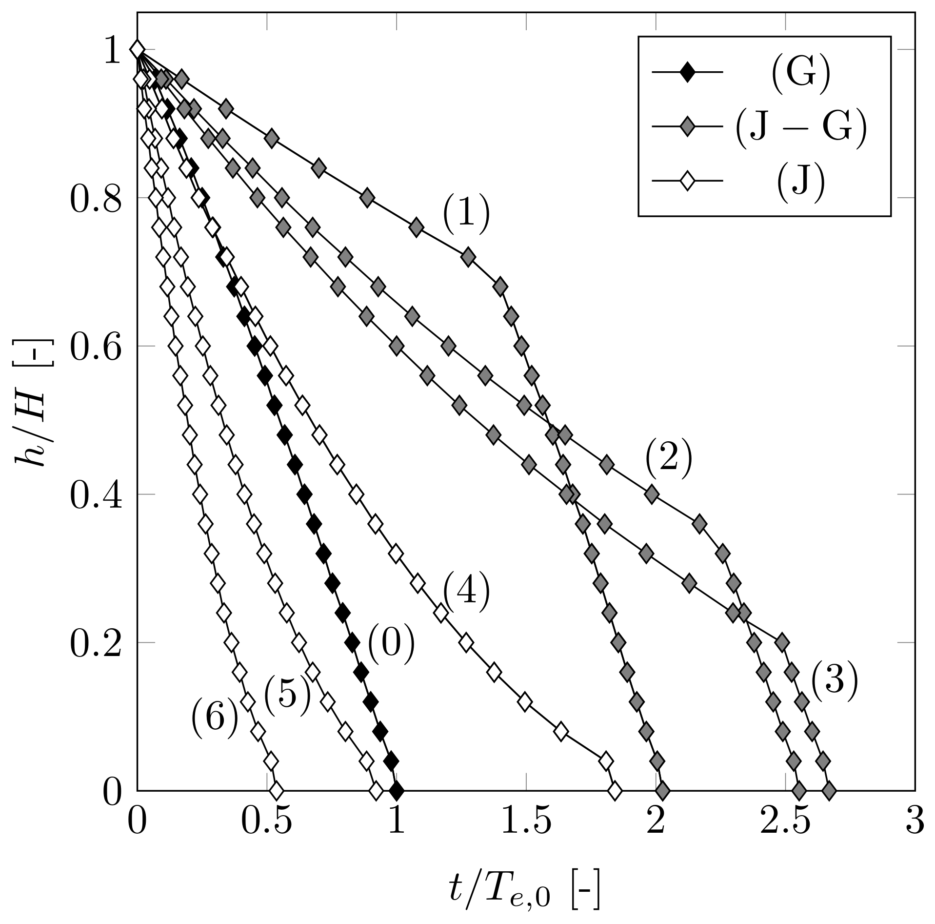
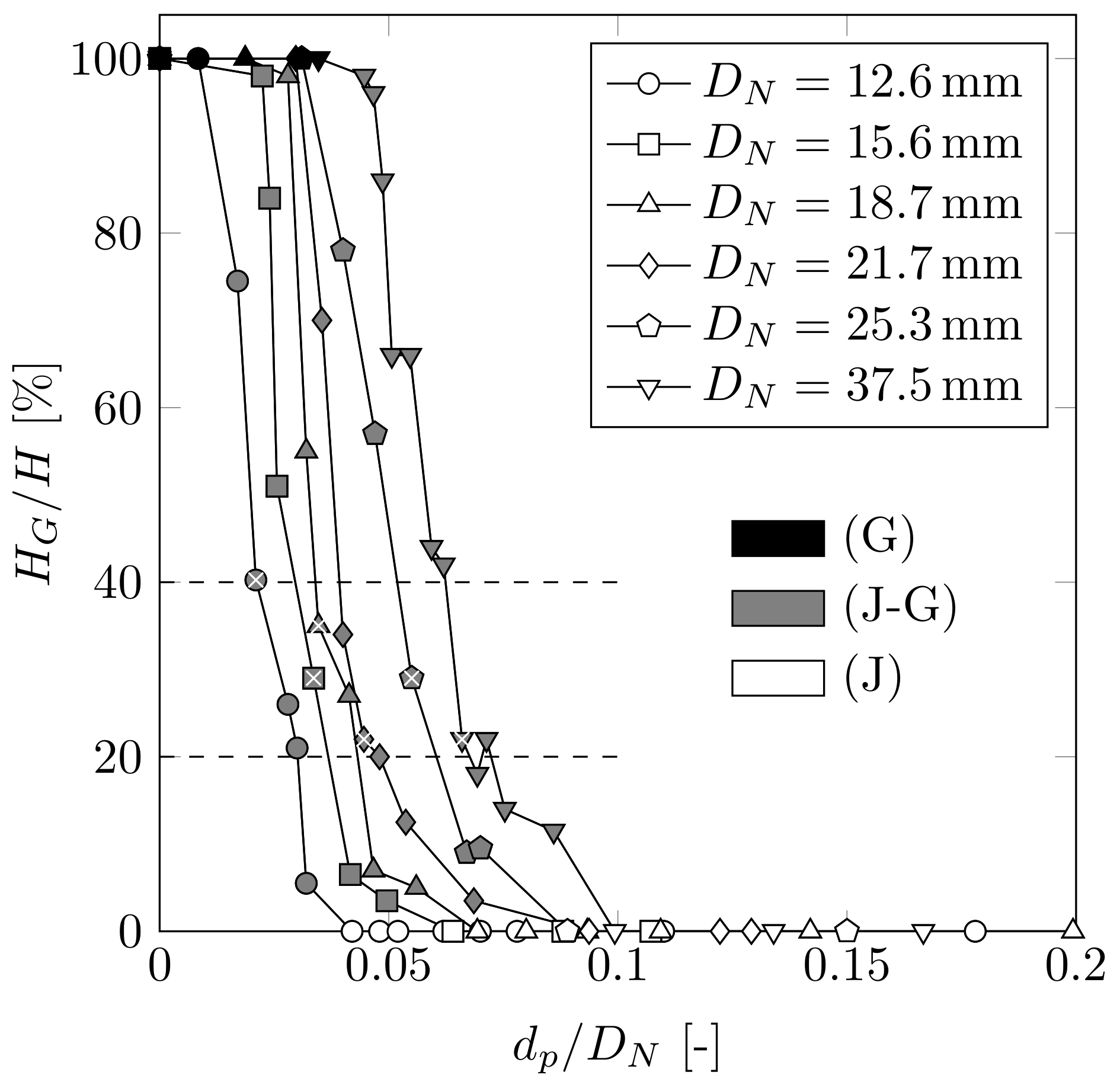
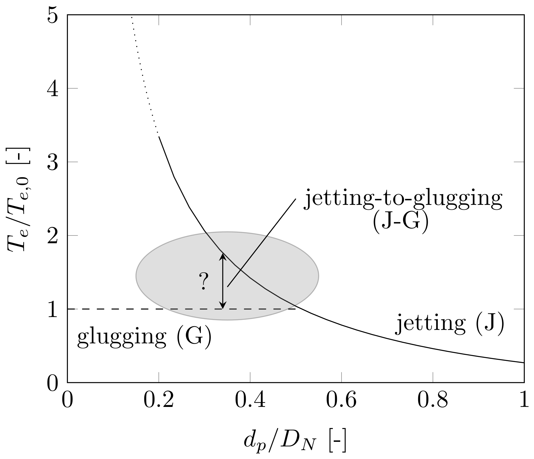
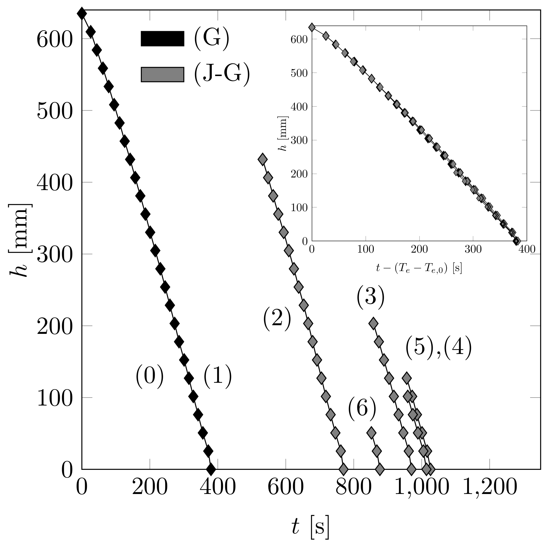
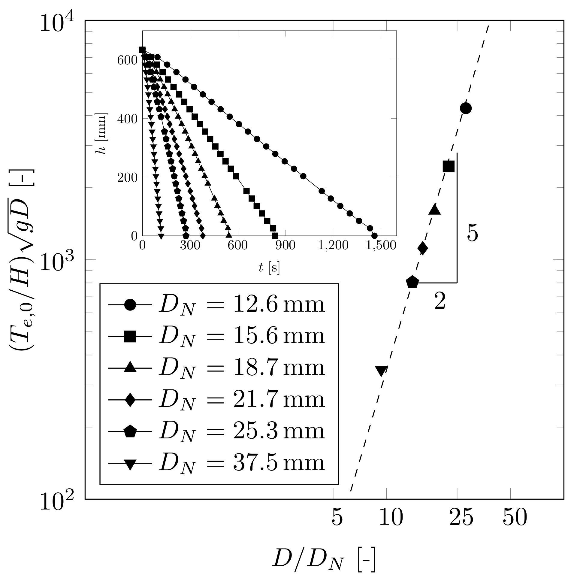
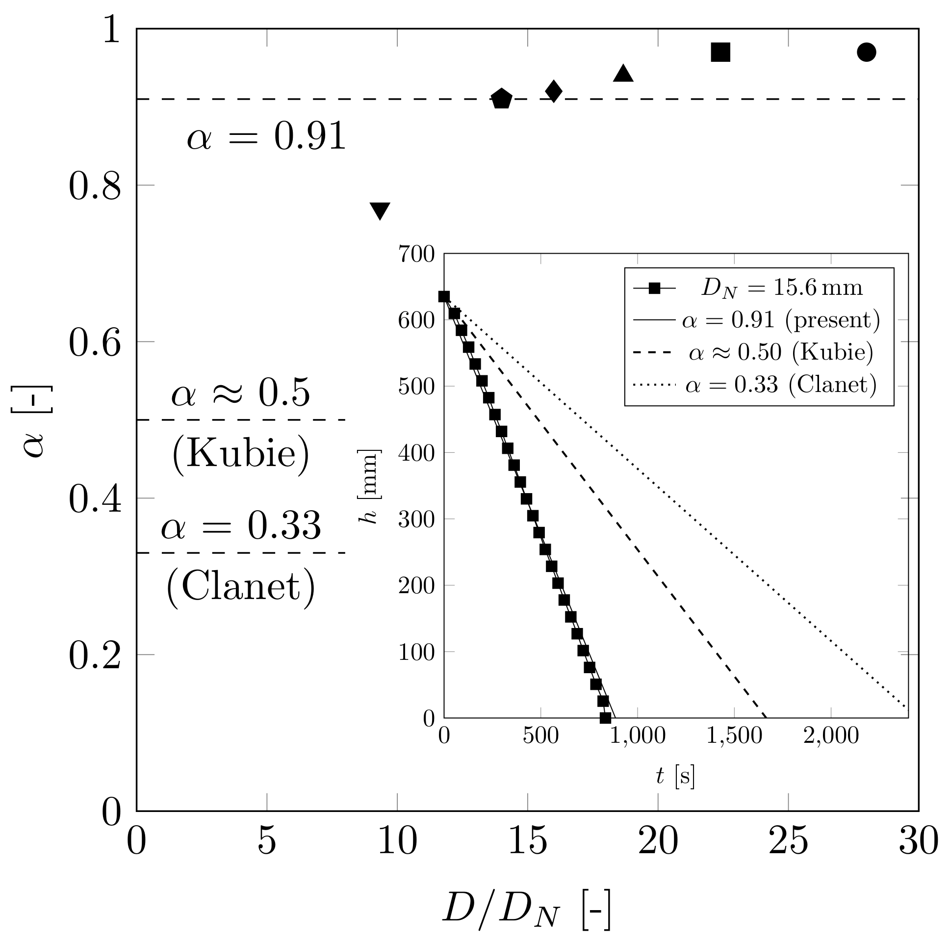
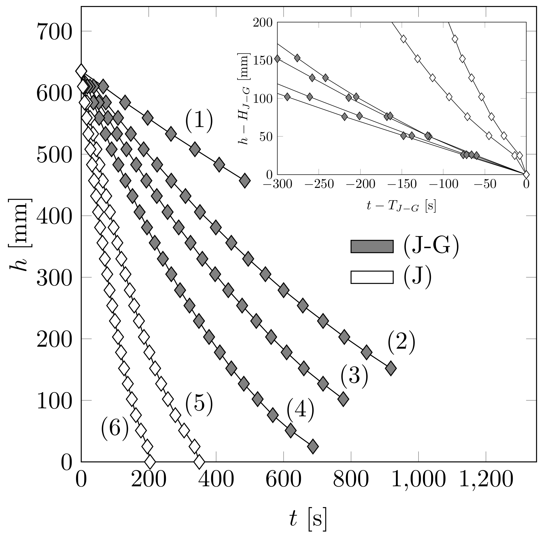
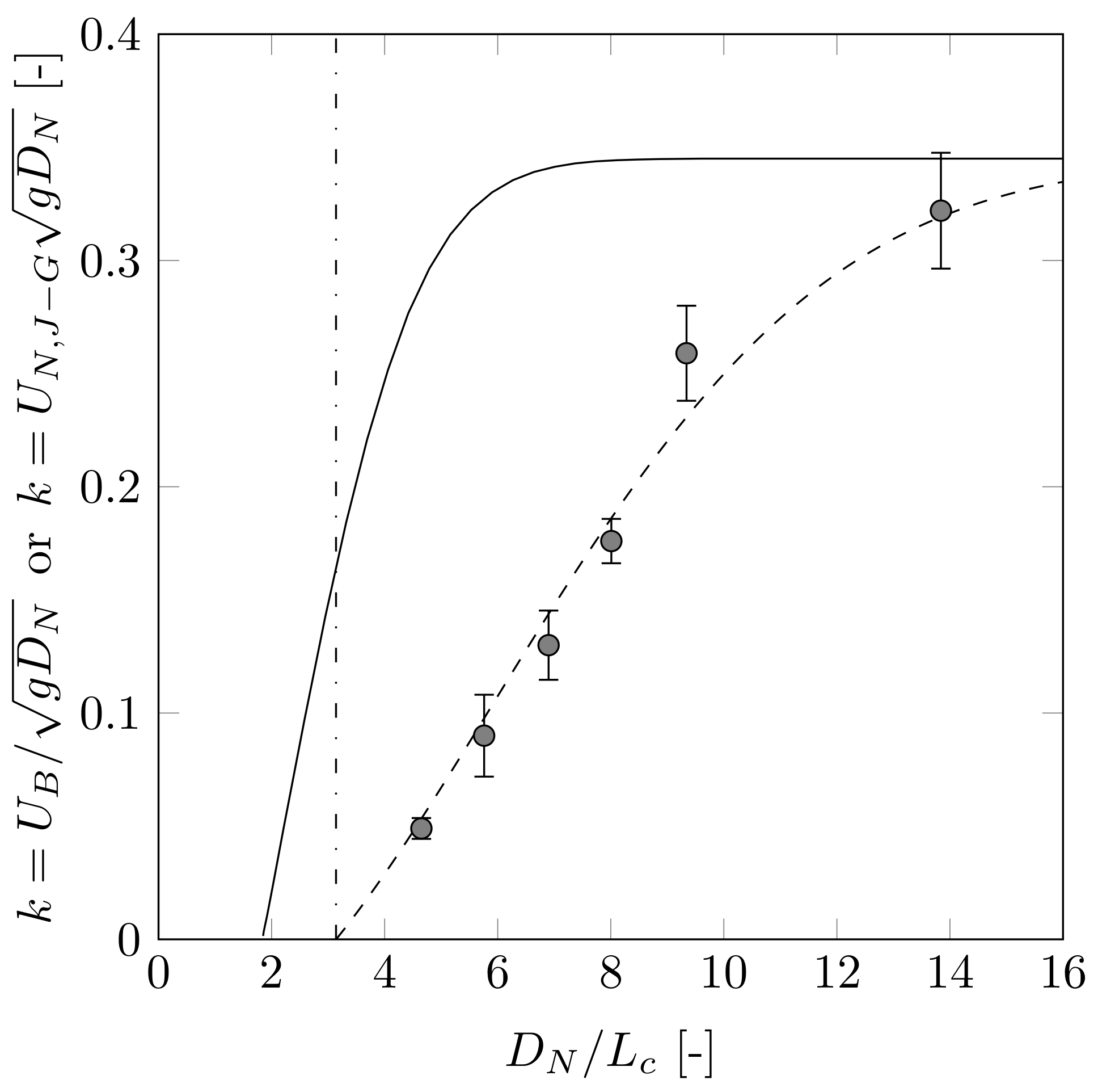
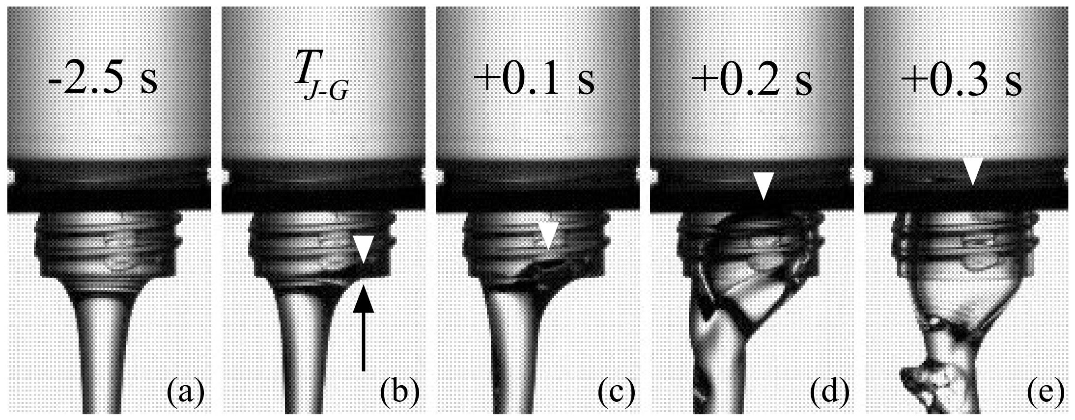
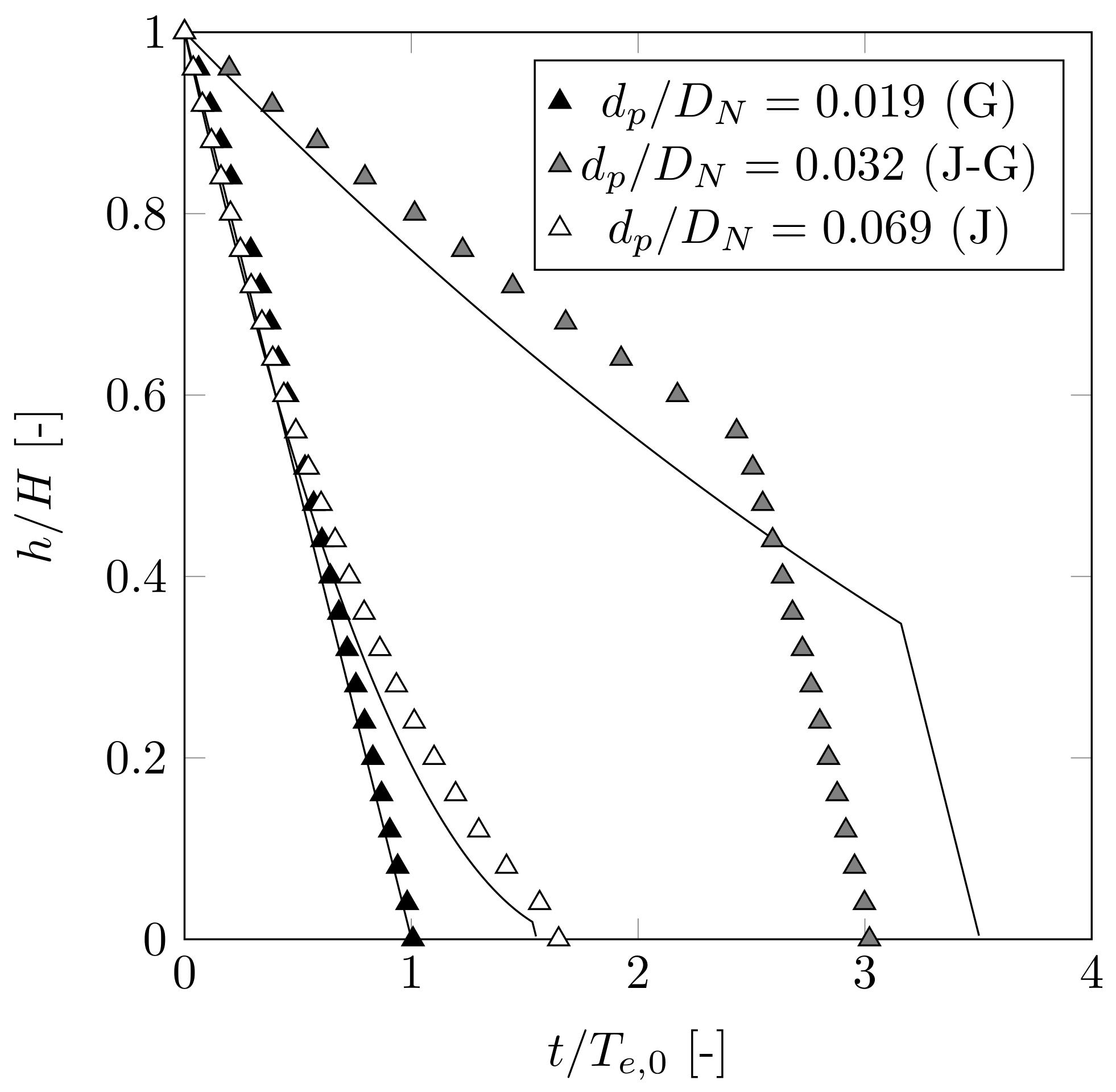
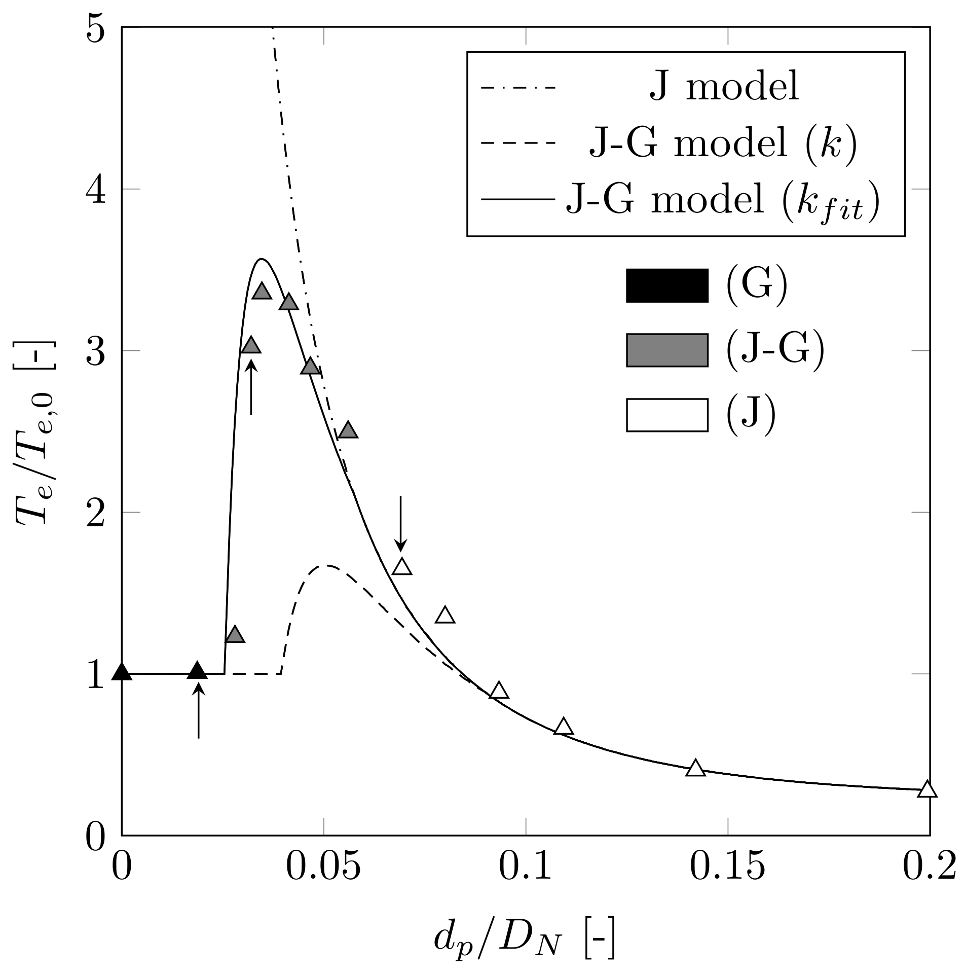
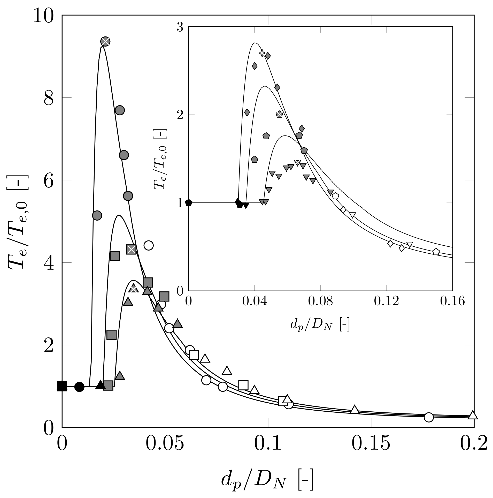
Table 1.
Neck and perforation diameters used for bottle emptying experiments ( and ). When including the experiments performed with , a total of 80 experiments were performed in this investigation. The provided ranges do not include values.
Table 1.
Neck and perforation diameters used for bottle emptying experiments ( and ). When including the experiments performed with , a total of 80 experiments were performed in this investigation. The provided ranges do not include values.
| Neck Diameter (Nominal) [mm] | Neck Diameter (Measured) [mm] | Perforation Diameter (Range) [mm] | Diameter Ratio (Range) [-] | Number of Perforations Tested [-] |
| 12.7 | 12.60.3 | 0.11–5.11 | 0.009–0.41 | 16 |
| 15.9 | 15.60.1 | 0.36–3.28 | 0.029–0.21 | 10 |
| 19.1 | 18.70.3 | 0.36–3.81 | 0.019–0.20 | 13 |
| 22.2 | 21.70.2 | 0.66–2.87 | 0.030–0.13 | 10 |
| 25.4 | 25.30.2 | 0.66–6.35 | 0.026–0.25 | 9 |
| 38.1 | 37.50.2 | 1.32–6.35 | 0.035–0.17 | 16 |
Table 2.
Range of emptying times and fraction of glugging height for the large bottle experiments. Uncertainty information for diameter and time values can be found in the Materials and Methods section. Ranges below diameter ratios and height ratios were determined from half the difference between the nominal and the bounding high–low values.
| [mm] | [s] | [s] | [-] | [-] | [%] |
| 12.6 | 1580 | 14730 | 9.4 | 0.021 | 40 |
| (0.019–0.025) | (33–58) | ||||
| 15.6 | 856 | 3693 | 4.3 | 0.034 | 29 |
| (0.030–0.038) | (18–40) | ||||
| 18.7 | 548 | 1838 | 3.4 | 0.035 | 35 |
| (0.034–0.039) | (31–45) | ||||
| 21.7 | 380 | 1026 | 2.7 | 0.045 | 22 |
| (0.043–0.047) | (21–28) | ||||
| 25.3 | 263 | 527 | 2.0 | 0.055 | 29 |
| (0.051–0.061) | (19–43) | ||||
| 37.5 | 118 | 172 | 1.5 | 0.066 | 22 |
| (0.065–0.069) | (20–32) |
Disclaimer/Publisher’s Note: The statements, opinions and data contained in all publications are solely those of the individual author(s) and contributor(s) and not of MDPI and/or the editor(s). MDPI and/or the editor(s) disclaim responsibility for any injury to people or property resulting from any ideas, methods, instructions or products referred to in the content. |
© 2023 by the authors. Licensee MDPI, Basel, Switzerland. This article is an open access article distributed under the terms and conditions of the Creative Commons Attribution (CC BY) license (https://creativecommons.org/licenses/by/4.0/).
Share and Cite
MDPI and ACS Style
Schwefler, C.; Nienaber, P.; Mayer, H.C. The Emptying of a Perforated Bottle: Influence of Perforation Size on Emptying Time and the Physical Nature of the Process. Fluids 2023, 8, 225. https://doi.org/10.3390/fluids8080225
AMA Style
Schwefler C, Nienaber P, Mayer HC. The Emptying of a Perforated Bottle: Influence of Perforation Size on Emptying Time and the Physical Nature of the Process. Fluids. 2023; 8(8):225. https://doi.org/10.3390/fluids8080225
Chicago/Turabian StyleSchwefler, Callen, Peyton Nienaber, and Hans C. Mayer. 2023. "The Emptying of a Perforated Bottle: Influence of Perforation Size on Emptying Time and the Physical Nature of the Process" Fluids 8, no. 8: 225. https://doi.org/10.3390/fluids8080225