
The Multicomponent Higher-Order Chen–Lee–Liu System: The Riemann–Hilbert Problem and Its N-Soliton Solution


College of Mathematics and Systems Science, Shandong University of Science and Technology, Qingdao 266590, China
*
Author to whom correspondence should be addressed.
†
These authors contributed equally to this work.
Fractal Fract. 2022, 6(6), 327; https://doi.org/10.3390/fractalfract6060327
Submission received: 15 May 2022
/
Revised: 7 June 2022
/
Accepted: 10 June 2022
/
Published: 13 June 2022
(This article belongs to the Topic Advances in Nonlinear Dynamics: Methods and Applications)
Abstract
:It is well known that multicomponent integrable systems provide a method for analyzing phenomena with numerous interactions, due to the interactions between their different components. In this paper, we derive the multicomponent higher-order Chen–Lee–Liu (mHOCLL) system through the zero-curvature equation and recursive operators. Then, we apply the trace identity to obtain the bi-Hamiltonian structure of mHOCLL system, which certifies that the constructed system is integrable. Considering the spectral problem of the Lax pair, a related Riemann–Hilbert (RH) problem of this integrable system is naturally constructed with zero background, and the symmetry of this spectral problem is given. On the one hand, the explicit expression for the mHOCLL solution is not available when the RH problem is regular. However, according to the formal solution obtained using the Plemelj formula, the long-time asymptotic state of the mHOCLL solution can be obtained. On the other hand, the N-soliton solutions can be explicitly gained when the scattering problem is reflectionless, and its long-time behavior can still be discussed. Finally, the determinant form of the N-soliton solution is given, and one-, two-, and three-soliton solutions as specific examples are shown via the figures.
1. Introduction
Many phenomena in natural science and engineering technology are nonlinear. These phenomena are complex and changeable, and cannot be described only with simple linear models. Therefore, nonlinear models can describe complex phenomena in daily life and scientific research more accurately than linear models, so as to reflect the nature of the relevant phenomena more accurately. As one type of nonlinear partial differential equations (nPDEs), the integrable equations have attracted more attention for their good properties [1,2,3]. In general, the integrable equations have their own Lax pair, Hamiltonian structure, and infinity symmetries. However, at the same time, it is very difficult to solve the exact solution of nPDEs due to the nonlinear term of the equation. In 1967, Gardner et al. proposed a new method for solving integrable equations—the inverse scattering method, which not only provided new concepts and methods for applied technology, but also had a profound impact on the development of mathematics [1]. The inverse scattering method uses the Lax pair of integrable systems and the spectral theory of ordinary differential equations to transform the Cauchy problem into a linear integral equation which can provide an explicit solution in the case of a degenerate kernel. However, when the kernel of the integral equation is non-degenerate, an explicit expression for the solution is hard to come by. In 1975, Shabat first used the RH method to study the spectral problem of integrable systems [4]. Compared with the classical inverse scattering method, the RH method has a wider application range, such as: for the second-order spectral problem, the generalized linear model (GLM) theory is equivalent to the RH method, but for the higher-order spectral problem, there is no GLM theory. Therefore, some parts of the inverse scattering problem need to be transformed into the RH problem. Most importantly, the long-time asymptotic properties of the non-soliton solution can be obtained by analyzing the RH problem [5]. Recently, scholars have studied the RH problem of many integrable equations, such as the Kundu–Eckhaus equation [6], the Wadati–Konno–Ichikawa equation [7], the derivative nonlinear Schrödinger equation [8], the quartic nonlinear Schrödinger equation [9], the vector modified Korteweg–de Vries equation [10], the focusing Hirota equation [11], and so on.
In particular, the nonlinear Schrödinger(NLS) equation and the derivative NLS equation are the most popular, and they are reduced from two different hierarchies, Ablowitz–Kaup–Newell–Sugar (AKNS) and Kaup–Newell (KN), respectively. The general formula of the derivative NLS equation can be written as [12]
which can be used to describe the propagation of short light pulses [13]. Equation (1) is reduced to the KN equation when [14], Equation (1) changes into the CLL equation when [15,16], and Equation (1) changes into the Gerdjikov–Ivanov (GI) equation when [17,18]. As three types of derivative NLS, they can be changed with a gauge transformation, CLL → KN → GI. From a physical point of view, the GI equation has a high-order nonlinear term, while the KN equation has a self-dispersion term. From a mathematical point of view, these are three types of equations which have their unique Lax pairs. Up to now, there have some studies of these three equations, which mainly focus on the construction of the solution and the long-time asymptotic analysis.
In this paper, a mHOCLL equation is derived with a third-order dispersion and quintic nonlinear term:
from a high-order hierarchy, where , and denotes the complex conjugate. When , it is a scalar equation, whose Liouville integrability and multi-Hamiltonian structure have been given in [19]. Afterwards, its corresponding N-soliton was also obtained via the RH problem. Furthermore, the rogue wave and the N-soliton are constructed under the non-zero condition [15,16]. Compared to the general CLL, the high-order system behaves differently due to the effect of the high-order dispersion. More importantly, the multicomponent system produces richer characteristics between the different components. In recent years, multicomponent systems have received more and more attention [20,21,22,23]. Feng et al. studied the integrable semi-discretization of a multicomponent short pulse equation [20]. Gerdjikov et al. constructed the Jost solutions and the minimal set of scattering data for the case of local and non-local reductions [21]. Marvan et al. constructed a point transformation between two integrable systems, the multicomponent Harry Dym equation and the multicomponent extended Harry Dym equation, that does not preserve the class of multi-phase solutions [22]. Therefore, we intend to study the multicomponent equations as well as their Hamiltonian structure. Given this, the RH problem is constructed to obtain the N-order soliton.
In this paper, we mainly study the construction of the mHOCLL equation and obtain its soliton solution through a special correlated RH problem. According to the RH method, there are generally two standard steps required to solve nPDEs [24,25,26,27]. One is that nPDEs be transformed into the RH problem on the complex plane; that is, nPDEs must be raised to the complex plane for consideration. The other one is that the unsolvable RH problem be transformed into a solvable RH problem by decomposing the jump matrix, the deformation integral path, etc.
This paper is structured as follows. Section 2 constructs the mHOCLL integrable system and its bi-Hamiltonian structure. Section 3 studies the analytical properties of the Jost solution and builds the RH problem associated with the mHOCLL system. Section 4 gives the formal solution when the RH problem is regular and the N-soliton solution when there is no reflection coefficient, and discusses its long-time asymptotic state. Then, the determinant form of the N-soliton solution is given and one-, two-, and three-soliton solutions as specific examples are shown via the figures. Section 5 is the conclusion.
2. Multicomponent Higher-Order Chen–Lee–Liu Integrable Hierarchies
The Lax pair of the scalar CLL system is well known and has been well studied, but the mHOCLL system is rarely studied. Therefore, in this section, we build a mHOCLL system and its bi-Hamiltonian structure which certifies that the constructed system is integrable.
Firstly, we extend the scalar potential to the vector potential and introduce a spectral problem as follows:
where denotes the spectral parameter, and is defined in Equation (2).
Then, a solution is considered as
where A is a scalar, , are two n-dimensional columns, is an matrix, and denotes matrix the transpose. Based on Equation (A2), we can obtain
Then, is written in the following form:
where
Then, we can obtain four recursion relations:
To obtain the mHOCLL system, we take a specific set of initial values
Then, we can obtain
Meanwhile, according to the recursion relations (8), we can know
where
Secondly, the Lax matrix is rewritten as
where the subscript represents the positive part of the polynomial with respect to , and is the modification term. Then, according to the compatibility condition, we gain and . Then, the mHOCLL hierarchies are gained using the zero-curvature equation, Equation (A4) in Appendix A:
where with
When , the mHOCLL hierarchy is transformed into the mHOCLL equation:
which can be reduced to the higher-order CLL equation as .
Then, we determine the Liouville integrability of the mHOCLL hierarchies (14) using bi-Hamiltonian structures which are presented by the trace identity or the variational identity [28,29,30]. It is easy to gain from the matrix and
According to the trace identity (A8), we have
Substituting
into Equation (17) yields
Plugging these into the trace identity, we find that , and thereby it is easy to have
where
Then, we obtain the bi-Hamiltonian structure of the mHOCLL system:
where the Hamiltonian pairs .
3. Riemann–Hilbert Problem
In this section, we construct the RH problem of the mHOCLL system, acquire the symmetries of some matrices, and discuss the time evolution of the time-dependent scattering coefficients.
Firstly, the Lax pairs of the mHOCLL system need to be rewritten as
with
where
Here, , are defined in Equation (7) and is defined in Equation (14). We can easily find that the tr, and thus we need an appropriate transformation to make tr. Let us take a kind of gauge transformation
where and . Then, Equations (22) and (23) are transformed into
with
where
Here,
When all the potentials rapidly vanish as , the asymptotic behavior is easy to obtain from Equations (26) and (27): . Then, we introduce a new function
which satisfies the canonical normalization , when . Substituting Equation (29) into Equations (22) and (23), it is easy to obtain
Consider a solution to Equations (36) and (37) of the form
where D and are independent of the spectral parameter . Substituting Equation (32) into Equations (36) and (37) and comparing the same order of , it is easy to know that D is diagonal and satisfies
According to the , and Equation (A4), we can know
Therefore, we can define D as
and then we introduce a new function which satisfies . Based on the asymptotic behavior of , it is evident that
Then, we can obtain from Equations (30) and (31)
where
The Jost solutions obey the constant asymptotic condition
when , respectively.
Based on the boundary conditions (38) and the method of variation of the parameters, Equation (36) can be transformed into the Volterra integral equations [5] as follows:
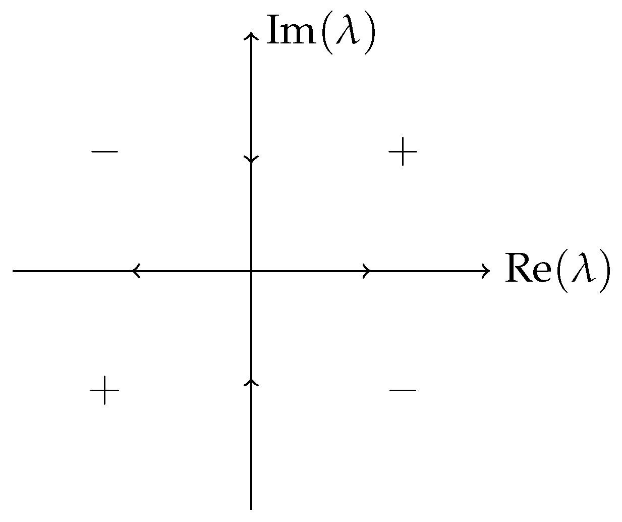
where and From Equation (39), it is evident that the first column of involves only the exponential factor . When is in , the first column of decays because of , and allows for analytical continuations to . Meanwhile, the last n columns of involve only the exponential factor . Therefore, when is in , they decay because of , and this allows for analytical continuations to the real and imaginary axis. Similarly, it is obvious that the last n columns of and the first column of are analytical in and analytically continued to (see Figure 1).
There is a linear relationship with matrix
because
are they are both solutions of Equation (22). Here, is the scattering matrix and satisfies det , and
It is easy to know that allows for analytic extension to , and are analytically extended to .
Then, we build two matrix eigenfunctions and make them continue analytically to and , respectively. We define as
Then, according to the analyticity of , we obtain
where and are defined by
is analytic in and continuous to . Substituting into Equation (40), it is evident that
Then,
The matrix eigenfunction which is analytic in has been constructed above. Now, we build the matrix eigenfunction which is analytic in , which need the adjoint matrix spectral problems
Due to det , the adjoint matrix . Similarly, we define as
Then, the corresponding matrix eigenfunction is written as
and
Here, , det, and is analytic in and continuous to .
According to the matrix functions , it is easy to obtain from Equations (40), (43), and (47)
where
Then, the generalized RH problem for the mHOCLL systems is expressed as
where denotes the jump contour.
Secondly, the symmetries of some matrices are considered. Due to , we can obtain the Hermitian equation of Equation (36):
where denotes the conjugate transpose. Combine Equations (45) and (51), and the properties of differential equations, and it is obvious that the involution relation is
Then, we obtain the involution property of through Equation (40):
The similar analysis shows that the Jost solutions the satisfy symmetry relation
where Then, it is easy to obtain
Next, we study the properties of and , which play an important role in a later analysis. From Equations (52) and (53), we obtain the following relations:
and
Based on the symmetry relation, we can know that if is a zero of , is another zero of . According to the involution relation, it is visible that has two zeros, namely, .
4. Solutions with the Riemann–Hilbert Method
In this section, we use the RH method to obtain the solutions to the mHOCLL system. There are two cases of the RH problem. One is the regular RH problem; the other is the non-regular RH problem.
Firstly, when the RH problem is regular, i.e., and , the explicit expression for the mHOCLL solution is not available, but we can obtain the formal solution obtained with the Plemelj formula. are introduced and used to rewrite the RH problem with the boundary condition
and
when . Then, according to Equation (48) and the Plemelj formula, we obtain
where and .
Suppose that and are two sets of solutions to Equation (58); then, , namely,
If and are analytic in and , respectively, a matrix function in the whole plane is defined by virtue of analytic continuation. According to Equation (59), this analytic function approaches the unit matrix when . In complex analysis, Liouville’s theorem tells that if a function is analytic and bounded in the entire complex plane, then this function must be a constant. Then, based on this theorem, it is easy to know that
in the whole plane. Thus, , which indicates that the solution is unique.
Secondly, we discuss the soliton solution for the RH problem with and . The uniqueness of the solutions to each associated RH problem (48) does not hold unless the zeros of det in are specified, and the structures of ker at those zeros are determined in [32,33,34].
From Equations (40), (43) and (47) it is visible that
According to the symmetry and involution relations of and , we suppose that has zeros , and has zeros . Here, we only discuss the case of a single zero; that is, all zeros and are simple. In this case, each of ker and ker only contain a single basis column vector and row vector, respectively. Then, it is easy to know that
According to [35,36,37], we know that the RH problem, which has the canonical normalization condition and zero structures in Equation (62), can be solved. When , we obtain ; that is, no reflection exists in the scattering problem. The solutions to this RH problem can be expressed as
where
with . Because the space part and time part are independent, we can easily obtain from Equation (36) and Equation (62)
If we combine this with Equation (62), we know that the vectors and have a linear relationship. Without loss of generality, we take the simplest case
Similarly, the time part of is taken as
In summary,
where is an arbitrary constant column.
Finally, is expanded at as
Substituting the above formula into Equation (36), it is easy to obtain
where . Equivalently,
From Equation (63), we obtain
If we combine Equations (72) and (73), the N-soliton solution of the mHOCLL system is obtained:
where the matrix is defined by Equation (64), and and , respectively.
4.1. N-Soliton Solution
In this subsection, we provide the specific expression and long-time asymptotic behavior of the N-soliton solution.
Firstly, according to , and Equations (64) and (68), if we take and
where
the solution in Equation (74) can be written as
where is the following matrix:
where the matrix is defined in Equation (64) with
Next, we provide the long-time asymptotic behavior of the N-soliton solution as . Since can be expressed as the adjoint matrix of divided by det , the N-soliton solution (77) is rewritten as
When , the asymptotic behavior of is given on the limit . Without loss of generality, assume .
In one case, according to the above assumption, it can be known that
when . Then, we consider the N region – with the following definitions, respectively:
The dominant terms contain the factor . Then, the numerator of with the factor is
and the denominator of is
Then, the asymptotic state of the solution (77) is
where ; is an odd number and is an even number.
The dominant terms contain the factor . With calculations similar to those in the case of , we obtain the asymptotic state of given by Equation (85) with .
In another case, it is easy to know that
when . Similarly, we consider the N region –, respectively.
The dominant terms contain the factor , and the asymptotic state is
where .
The dominant terms contain the factor , and the asymptotic state is
where .
The dominant terms contain the factor . With calculations similar to those in the case , we obtain the asymptotic form of given by Equation (88) with .
If we combine Equations (84) and (85), or Equations (87) and (88), it is easy to obtain the following theorem.
Theorem 1.
The long-time asymptotic states of the N-soliton solution of the n-th mHOCLL system are as follows (see Figure 2):
when
when
where
with ; is an odd number and is an even number.
Theorem 1 defines the collision laws of N-solitons in the n-th mHOCLL system.
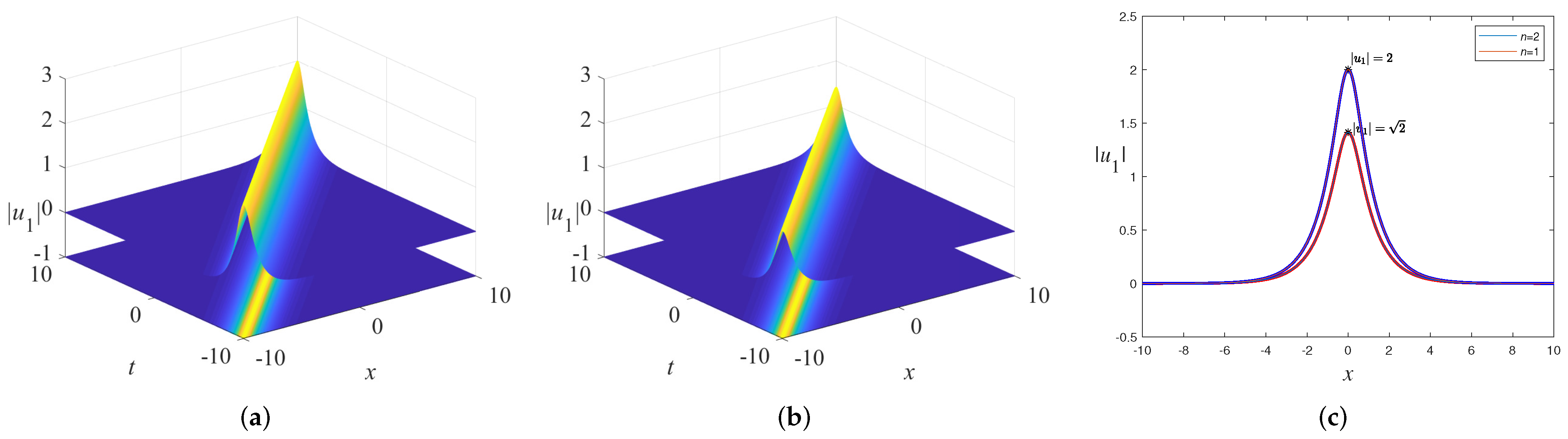
4.2. One-Soliton Solutions
When , the solution (77) is
Letting
we can rewrite Equation (91) as
where and are real parameters, , is odd number, and is even number. Without loss of generality, we give two cases of a one-soliton solution in Figure 3.
From Figure 3, we can see that the amplitude of the solitary wave decreases as n increases. Its peak amplitude and velocity are , and , respectively. The phase of the solution is linearly related to space x and time . The spatial gradient of the phase is proportional to the wave velocity.
4.3. Two-Soliton Solution
According to the factor of the exponential function in Equations (77)–(79), we can know that there are two different states of the two-soliton solution. One is , the other one is . Without loss of generality, we take
which makes the two-soliton solution elastically collide as shown in Figure 4a. Similarly, when we take
the two-soliton solution appears in the bound state shown in Figure 4b. Note that we only provide the figures for with .
From Figure 4a, it can be seen that when , the solution contains two single-solitons which are far apart and moving toward each other as . When they collide, they interact strongly. However, when , they reappear from the interaction without changing shape or velocity; that is, no energy radiation is emitted into the far field. Hence, the interactions of the solitons are elastic. The elastic collision is one of the most important characteristics of solitary waves, which can indicate that the mHOCLL system (22) is integrable. However, although the elastic collision occurs, it will inevitably leave some collision marks. From Figure 4, we can see that after the collision, each soliton is position-shifted and phase-shifted.
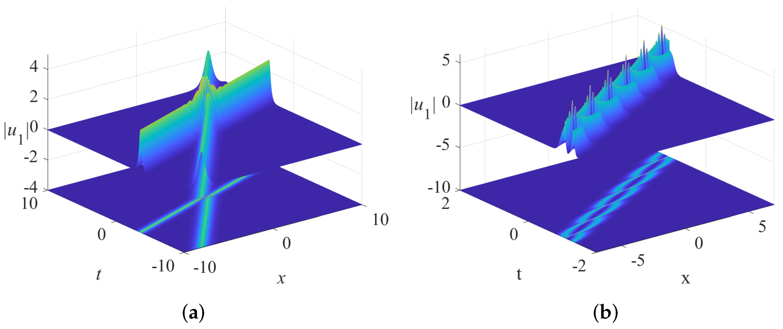
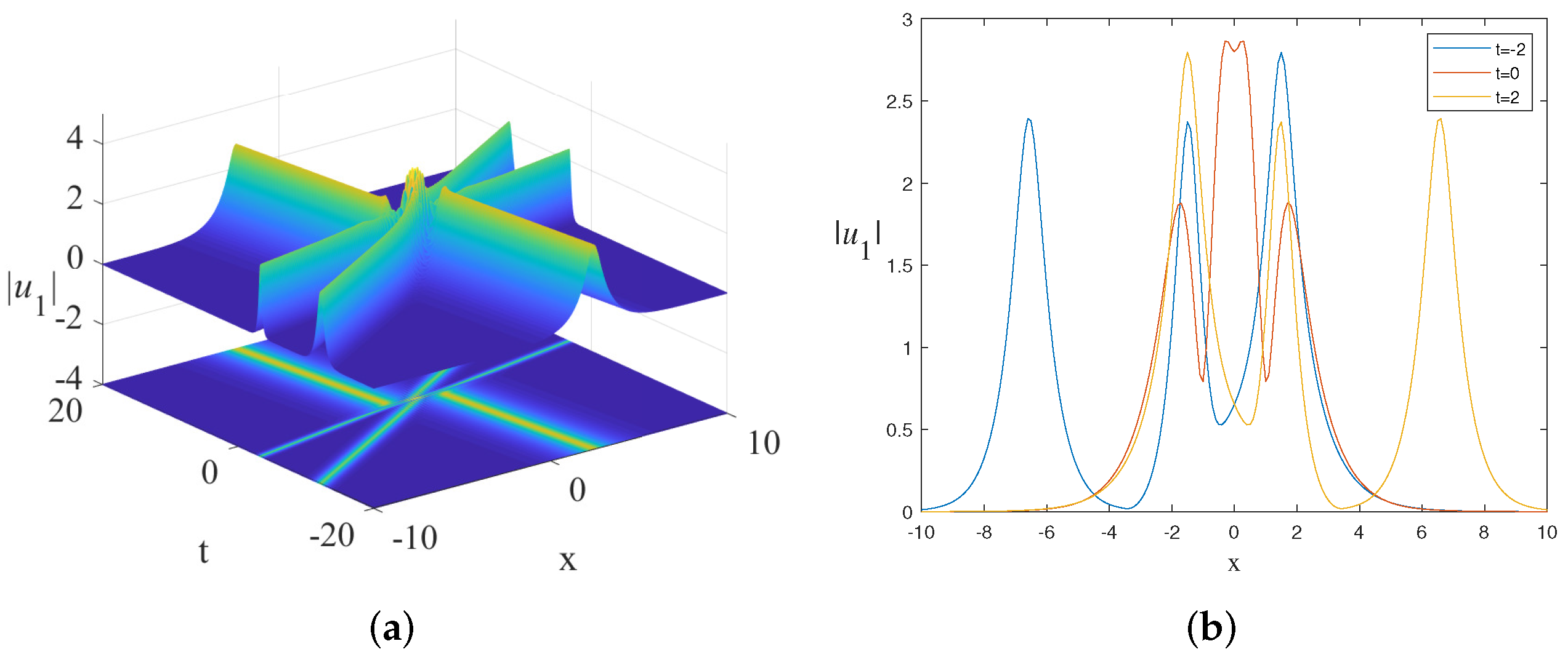
4.4. Three-Soliton Solution
Take
we give the figures of three-soliton solution in Figure 5.
5. Conclusions
In this paper, an arbitrary order matrix spectral problem was used to generate the mHOCLL system. Meanwhile, the bi-Hamiltonian structure of this system was given by the trace identity. Then, the corresponding RH problem was constructed with zero background. To obtain the exact solution of the system, we discussed two cases of the RH problem. One was that the RH problem is regular. The other one was that the RH problem is non-regular and the scattering problem is reflectionless. When the jump matrix J was an identity matrix, the N-soliton solution of the mHOCLL system presented the explicit formulas, and its long-time asymptotic behavior was analyzed. Finally, we provided the determinant form of the N-soliton solution and the figures of one-, two-, three-soliton solutions as specific examples.
The RH method is a very efficient method for obtaining soliton solutions. We obtained some results in this paper and we look forward to studying multicomponent systems, which include different Lie algebras [38], quadratic spectral parameters [21,39,40], and polynomial spectral parameters [41]. In addition, we will investigate where the jump matrix can be obtained at non-zero boundary branch cuts and use the RH method to obtain rogue waves. Our results from the perspective of the RH method will hopefully be of great help in studying the exact solutions of integrable equations.
Author Contributions
Conceptualization, H.D.; methodology, Y.F.; software, Y.Z.; validation, Y.Z., H.D. and Y.F.; formal analysis, H.D.; resources, Y.F.; writing—original draft preparation, H.D. and Y.Z.; writing—review and editing, Y.F.; visualization, Y.Z. All authors have read and agreed to the published version of the manuscript.
Funding
The research is funded by the National Natural Science Foundation of China (No. 11975143, 12105161, 61602188), the Shandong Provincial Natural Science Foundation (No. ZR2019QD018), and the Scientific Research Foundation of Shandong University of Science and Technology for Recruited Talents (No. 2017RCJJ068, 2017RCJJ069).
Institutional Review Board Statement
Not applicable.
Informed Consent Statement
Not applicable.
Data Availability Statement
Not applicable.
Acknowledgments
Thanks to the editors and reviewers for their great contributions to the improvement of the paper.
Conflicts of Interest
The authors declare no conflict of interest.
Appendix A. Zero-Curvature Method
The zero-curvature method is a very efficient way to construct an integrable hierarchy. It mainly uses the spectral matrix and the matrix to be solved, where can be generated from loop algebras, and Lie algebras can be semi-simple [28] or non-semi-simple [30].
Introduce a matrix
where is a potential vector and is the spectral parameter. In order to solve the matrix , we need to obtain the recursion relation of the parameters via the stationary zero-curvature equation
When we obtain the recursion relation, if we give an initial matrix , we can obtain a unique matrix . From the matrix , we generate a series of Lax matrices
Through the zero-curvature equation
we can obtain and integrable hierarchies
where the matrices and are a Lax pair of integrable systems [42]. Therefore, it can be expressed as spatial and temporal spectral problems
where is a matrix eigenfunction, and their compatibility condition is zero-curvature Equation (A4).
Then, we construct the bi-Hamiltonian structure to analyze Equation (A5)’s Liouville integrability [43]:
where and are Hamiltonian pairs and denotes the variational derivative [44]. We usually use the trace identification [28]
or the variational identity [30]
to obtain the Hamiltonian structure. Here, is a symmetric, ad-invariant, and non-degenerate bilinear form. The bi-Hamiltonian structure ensures conserved quantities and infinite commutative Lie symmetry
where or , and means the Gateaux derivative of K with respect to .
For an integrable equation with potential functions, we know that is a conserved functional, iff is an adjoint symmetry [29]. Therefore, the existence of adjoint symmetry is necessary to permit conservation laws for systems of completely non-degenerate differential equations, and a pair of symmetry and adjoint symmetry creates the conservation laws of differential equations [45].
References
- Gardner, C.S.; Greene, J.M.; Kruskal, M.D.; Miura, R.M. Method for solving the Korteweg-de Vries equation. Phys. Rev. Lett. 1967, 19, 1095. [Google Scholar] [CrossRef]
- Zakharov, V.E.; Shabat, A.B. Exact theory of two-dimensional self-focusing and one-dimensional self-modulation of waves in nonlinear media. Sov. Phys. JETP 1972, 34, 62–69. [Google Scholar]
- Date, E.; Jimbo, M.; Kashiwara, M.; Miwa, T. KP hierarchies of orthogonal and symplectic type-transformation groups for soliton equations VI. J. Phys. Soc. Jpn. 1981, 50, 3813–3818. [Google Scholar] [CrossRef]
- Shabat, A.B. Inverse-scattering problem for a system of differential equations. Funct. Anal. Appl. 1975, 9, 244–247. [Google Scholar] [CrossRef]
- Novikov, S.P.; Manakov, S.V.; Pitaevskii, L.P.; Zakharov, V.E. Theory of Solitons: The Inverse Scattering Method; Consultants Bureau: New York, NY, USA, 1984. [Google Scholar]
- Wang, D.S.; Wang, X.L. Long-time asymptotics and the bright-soliton solutions of the Kundu-Eckhaus equation via the Riemann-Hilbert approach. Nonlinear Anal. Real. 2018, 41, 334–361. [Google Scholar] [CrossRef]
- Zhang, Y.S.; Rao, J.G.; Cheng, Y.; He, J.S. Riemann-Hilbert method for the Wadati-Konno-Ichikawa equation: Simple poles and one higher-order pole. Phys. D Nonlinear Phenom. 2019, 399, 173–185. [Google Scholar] [CrossRef]
- Zhao, P.; Fan, E.G. Finite gap integration of the derivative nonlinear Schrödinger equation: A Riemann-Hilbert method. Phys. D Nonlinear Phenom. 2020, 402, 132213. [Google Scholar] [CrossRef]
- Liu, N.; Guo, B.L. Solitons and rogue waves of the quartic nonlinear Schrödinger equation by Riemann-Hilbert approach. Nonlinear Dyn. 2020, 100, 629–646. [Google Scholar] [CrossRef]
- Wang, X.B.; Han, B. Application of the Riemann-Hilbert method to the vector modified Korteweg-de Vries equation. Nonlinear Dyn. 2020, 99, 1363–1377. [Google Scholar] [CrossRef]
- Zhang, X.F.; Tian, S.F.; Yang, J.J. The Riemann-Hilbert approach for the focusing Hirota equation with single and double poles. Anal. Math. Phys. 2021, 11, 86. [Google Scholar] [CrossRef]
- Hisakado, M.; Wadati, M. Integrable multi-component hybrid nonlinear Schrödinger equations. J. Phys. Soc. Jpn. 1995, 64, 408–413. [Google Scholar] [CrossRef]
- Mio, K.; Ogino, T.; Minami, K.; Takeda, S. Modulational instability and envelope-solitons for nonlinear Alfvén waves propagating along the Magnetic field in Plasmas. J. Phys. Soc. Jpn. 1976, 41, 667–673. [Google Scholar] [CrossRef]
- Xu, S.W.; He, J.S.; Wang, L.H. The darboux transformation of the derivative nonlinear Schrödinger equation. J. Phys. A Math. Theor. 2011, 44, 305203. [Google Scholar] [CrossRef] [Green Version]
- Zhang, J.; Liu, W.; Qiu, D.Q.; Zhang, Y.S.; Porsezian, K.; He, J.S. Rogue wave solutions of a higher-order Chen-Lee-Liu equation. Phys. Scripta 2015, 90, 055207. [Google Scholar] [CrossRef]
- Zhao, Y.; Fan, E.G. N-soliton solution for a higher-order Chen-Lee-Liu equation with nonzero boundary conditions. Mod. Phys. Lett. B 2020, 34, 2050054. [Google Scholar] [CrossRef]
- Gerdjikov, V.S.; Ivanov, M.I. The quadratic bundle of general form and the nonlinear evolution equations. Bulg. J. Phys. 1983, 10, 1–16. [Google Scholar]
- Fan, E.G. Darboux transformation and soliton-like solutions for the Gerdjikov-Ivanov equation. J. Phys. A Math. Gen. 2000, 33, 6925. [Google Scholar] [CrossRef]
- Fan, E.G. A family of completely integrable multi-hamiltonian systems explicitly related to some celebrated equations. J. Math. Phys. 2001, 42, 4327. [Google Scholar] [CrossRef]
- Feng, B.F.; Maruno, K.; Ohta, Y. Integrable semi-discretization of a multi-component short pulse equation. J. Math. Phys. 2015, 56, 043502. [Google Scholar] [CrossRef] [Green Version]
- Gerdjikov, V.S.; Grahovski, G.G.; Ivanov, R.I. On integrable wave interactions and Lax pairs on symmetric spaces. Wave Motion 2017, 71, 53–70. [Google Scholar] [CrossRef] [Green Version]
- Marvan, M.; Pavlov, M.V. A new class of solutions for the multi-component extended Harry Dym equation. Wave Motion 2017, 74, 151–158. [Google Scholar] [CrossRef] [Green Version]
- Li, Y.; Li, J.; Wang, R.Q. Multi-soliton solutions of the N-component nonlinear Schrödinger equations via Riemann–Hilbert approach. Nonlinear Dyn. 2021, 105, 1765–1772. [Google Scholar] [CrossRef]
- Zakharov, V.E.; Shabat, A.B. Integration of the nonlinear equations of mathematical physics by the method of inverse scattering II. Funct. Anal. Appl. 1979, 13, 166–174. [Google Scholar] [CrossRef]
- Doktorov, E.V.; Leble, S.B. A Dressing Method in Mathematical Physics. In Mathematical Physics Studies; Springer: Dordrecht, The Netherlands, 2007. [Google Scholar]
- Gerdjikov, V.S.; Vilasi, G.; Yanovski, A.B. Integrable Hamiltonian Hierarchies: Spectral and Geometric Methods; Springer: Berlin/Heidelberg, Germany, 2008. [Google Scholar]
- Ma, W.X. Application of the Riemann-Hilbert approach to the multicomponent AKNS integrable hierarchies. Nonlinear Anal. Real World Appl. 2019, 47, 1–17. [Google Scholar] [CrossRef]
- Tu, G.Z.; Meng, D.Z. The trace identity, a powerful tool for constructing the Hamiltonian structure of integrable systems (II). Acta Math. Appl. Sin. 1989, 5, 89–96. [Google Scholar] [CrossRef]
- Ma, W.X.; Zhou, R.G. Adjoint symmetry constraints leading to binary nonlinearization. J. Nonlinear Math. Phy. 2002, 9, 106–126. [Google Scholar] [CrossRef] [Green Version]
- Ma, W.X.; Chen, M. Hamiltonian and quasi-Hamiltonian structures associated with semi-direct sums of Lie algebras. J. Phys. A Math. Gen. 2006, 39, 10787–10801. [Google Scholar] [CrossRef] [Green Version]
- Fuchssteiner, B.; Fokas, A.S. Symplectic structures, their Ba¨cklund transformations and hereditary symmetries. Phys. D Nonlinear Phenom. 1981, 4, 47–66. [Google Scholar] [CrossRef]
- Shchesnovich, V.S. Perturbation theory for nearly integrable multicomponent nonlinear PDEs. J. Math. Phys. 2002, 43, 1460–1486. [Google Scholar] [CrossRef] [Green Version]
- Shchesnovich, V.S.; Yang, J.K. General soliton matrices in the Riemann-Hilbert problem for integrable nonlinear equations. J. Math. Phys. 2003, 44, 4604–4639. [Google Scholar] [CrossRef] [Green Version]
- Yang, J.K. Nonlinear Waves in Integrable and Nonintegrable Systems; SIAM: Philadelphia, PA, USA, 2010. [Google Scholar]
- Lenells, J. Dressing for a novel integrable generalization of the nonlinear Schrödinger equation. J. Nonlinear Sci. 2010, 20, 709–722. [Google Scholar] [CrossRef] [Green Version]
- Guo, B.L.; Ling, L.M. Riemann-Hilbert approach and N-soliton formula for coupled derivative Schrödinger equation. J. Math. Phys. 2012, 53, 073506. [Google Scholar] [CrossRef]
- Kawata, T. Riemann Spectral Method for the Nonlinear Evolution Equations; Cambridge University Press: Cambridge, UK, 1984. [Google Scholar]
- Gerdjikov, V.S. Algebraic and analytic aspects of soliton type equations. Ann. Phys. 2002, 301, 35–68. [Google Scholar]
- Gerdzhikov, V.S.; Ivanov, M.I.; Kulish, P.P. Quadratic bundle and nonlinear equations. Theor. Math. Phys. 1980, 44, 784–795. [Google Scholar] [CrossRef]
- Valchev, T.I. Dressing method and quadratic bundles related to symmetric spaces. Vanishing boundary conditions. J. Math. Phys. 2016, 57, 021508. [Google Scholar] [CrossRef] [Green Version]
- Gerdjikov, V.S.; Ivanov, R.I.; Stefanov, A.A. Riemann-Hilbert problem, integrability and reductions. J. Geom. Mech. 2019, 11, 167–185. [Google Scholar] [CrossRef] [Green Version]
- Lax, P.D. Integrals of nonlinear equations of evolution and solitary waves. Commun. Pur. Appl. Math. 1968, 21, 467–490. [Google Scholar] [CrossRef]
- Magri, F. A simple model of the integrable Hamiltonian equation. J. Math. Phys. 1978, 19, 1156. [Google Scholar] [CrossRef]
- Ma, W.X.; Fuchssteiner, B. Integrable theory of the perturbation equations. Chaos Soliton. Fract. 1996, 7, 1227–1250. [Google Scholar] [CrossRef] [Green Version]
- Drinfel’d, V.G.; Sokolov, V.V. Lie algebras and equations of Korteweg-de Vries type. J. Soviet Math. 1985, 30, 1975–2036. [Google Scholar] [CrossRef]
Figure 1.
The jump contour in the complex -plane.

Figure 2.
N-soliton collision in the n-th mHOCLL system.

Figure 3.
One-soliton solutions to the mHOCLL system: (a) ; (b) ; (c) when , the comparison of the two cases.
Figure 3.
One-soliton solutions to the mHOCLL system: (a) ; (b) ; (c) when , the comparison of the two cases.

Figure 4.
Two-soliton solutions to the mHOCLL system: (a) collision, where ; (b) bound stste, where .
Figure 4.
Two-soliton solutions to the mHOCLL system: (a) collision, where ; (b) bound stste, where .

Figure 5.
Three-soliton solutions to the mHOCLL system with : (a) 3D image; (b) plane diagrams at three different times.
Figure 5.
Three-soliton solutions to the mHOCLL system with : (a) 3D image; (b) plane diagrams at three different times.

Publisher’s Note: MDPI stays neutral with regard to jurisdictional claims in published maps and institutional affiliations. |
© 2022 by the authors. Licensee MDPI, Basel, Switzerland. This article is an open access article distributed under the terms and conditions of the Creative Commons Attribution (CC BY) license (https://creativecommons.org/licenses/by/4.0/).
Share and Cite
MDPI and ACS Style
Zhang, Y.; Dong, H.; Fang, Y. The Multicomponent Higher-Order Chen–Lee–Liu System: The Riemann–Hilbert Problem and Its N-Soliton Solution. Fractal Fract. 2022, 6, 327. https://doi.org/10.3390/fractalfract6060327
AMA Style
Zhang Y, Dong H, Fang Y. The Multicomponent Higher-Order Chen–Lee–Liu System: The Riemann–Hilbert Problem and Its N-Soliton Solution. Fractal and Fractional. 2022; 6(6):327. https://doi.org/10.3390/fractalfract6060327
Chicago/Turabian StyleZhang, Yong, Huanhe Dong, and Yong Fang. 2022. "The Multicomponent Higher-Order Chen–Lee–Liu System: The Riemann–Hilbert Problem and Its N-Soliton Solution" Fractal and Fractional 6, no. 6: 327. https://doi.org/10.3390/fractalfract6060327