Article

Spatial and Paleoclimatic Reconstruction of the Peña Negra Paleoglacier (Sierra de Béjar-Candelario, Spain) during the Last Glacial Cycle (Late Pleistocene)

by
Carlos E. Nieto
,
Ana Calvo
,
Raquel Cruz
,
Antonio Miguel Martínez-Graña
,
José Luis Goy
and
José Ángel González-Delgado
*
Department of Geology, Faculty of Sciences, Merced Square, University of Salamanca, 37008 Salamanca, Spain
*
Author to whom correspondence should be addressed.
Sustainability 2023, 15(23), 16514; https://doi.org/10.3390/su152316514
Submission received: 3 November 2023 / Revised: 29 November 2023 / Accepted: 1 December 2023 / Published: 3 December 2023

Abstract

:
The study of the Peña Negra paleoglacier during the Last Glacial Maximum reveals its sensitivity to paleoclimatic variations. The evolutionary phases of the paleoglacier are correlated with the evolutionary models proposed for the Sierra de Béjar-Candelario and the Central Iberian System. To recognize the mechanisms of ice advance/retreat and the response of the glacier to paleoclimatic variations, modeling is carried out based on a geographic information system tool. This model is key to establishing the spatial extent of the ice and the estimation of the Equilibrium line altitudeequilibrium line altitudes at each moment, which makes it easier to infer the approximate climatic conditions of each phase (temperature and precipitation) and allows us to improve the understanding of the glacial dynamics versus variations in paleoenvironmental conditions and paleoglacial morphometry. The spatial reconstruction data show that the paleoglacier had 0.526 km3 of ice during the phase of maximum extension, while the paleoclimatic data reflect an increase in precipitation and a slight decrease in average summer temperatures compared to today. The stability phases are associated with the periods of greatest precipitation when the mass balance was positive.

1. Introduction

The successive climatic changes during the recent Late Pleistocene played a significant role in the glacial development of the mountains in southern Europe [1] and in their current landscapes. Abundant marine sedimentary records bordering the Iberian Peninsula reflect the region’s susceptibility to North Atlantic climatic changes [2]. These climatic variations are well documented in all mountain ranges and massifs. The major mountain chains preserve a valuable record of past glaciation, primarily linked to the Last Glacial Cycle (LGC).
Glacial landscapes have been a subject of research since the 19th century and have gained particular attention in recent decades. This research aims to comprehend the timing, extent, and complexity of the Quaternary glaciation concerning past climatic changes and oceanic and atmospheric circulation patterns. Investigations have led to detailed and robust cartography, focusing on the main mountain chains and massifs, as well as specific valleys. Morphostratigraphic sequences and existing chronologies based on dating of 14C, OSL, 14Be, Cl and Ne indicate four significant advances primarily centered on MIS 4–MIS 2, though these advances vary in extent and are not uniformly identified in some specific sectors or valleys. The northernmost sector of the Iberian Peninsula (Cantabrian Cordillera and Pyrenees) experienced extensive glaciation with multiple fluctuations, related to pronounced southward shifts in the polar front, which directed moist masses from the Atlantic towards the continent, driven by the westerly winds (a significant component of atmospheric circulation at these latitudes). Detailed cartography and chronologies have allowed the reconstruction of two major advances related to the Middle European Glaciation (MIS 4–MIS 3) and the Last Glacial Maximum (MIS 2), followed by a progressive retreat during the Late Glacial period. This period records two significant pulses, one centered on the Older Dryas during a cold/dry episode initiated during a period of weak Atlantic Meridional Overturning Circulation (AMOC) and another during the Younger Dryas, which is only recorded in the highest cirques [3]. In the Sierra de Gredos (central sector of the Iberian Peninsula), this last glaciation was important, with extensive MIS 2 glaciers affecting its peaks [4,5,6,7]. This northeast-to-southwest-oriented range is also influenced by westerly winds. Glacial research began in the late 19th century [8,9] and developed substantially in the 20th and early 21st centuries, resulting in detailed descriptions, cartography, and models regarding the evolution of glaciers during the LGC [10,11,12,13,14]. In recent decades, research has focused on establishing chronologies, environments, and ice mass reconstructions [15,16,17].
The Sierra de Béjar-Candelario (the westernmost sector of Gredos in the southeastern region of the province of Salamanca, Spain) was notably affected by these climatic changes, particularly during the LGC, which shaped its landscapes. During cold periods (glacials and/or stadials) of this cycle, ice accumulation on the hills, cirques, and glacial valleys led to significant erosive actions, resulting in cirque incisions (escarpments) and valley-side step features, as well as the deposition of moraines at the margins of the glacial valleys, both in front of and behind the ice cap. During warm periods (interglacials and/or interstadials), the ice melted, leaving behind englacial and supraglacial materials on the valley floor moraines and river incision in the fluvial valleys. Detailed cartography [13] has enabled the separation of moraine sequences in the cirques and glacial valleys, providing a general relative chronosequence for the study area during Late Pleistocene moments. The geometrical and spatial characteristics of these glacial deposits have also allowed for the differentiation of four key stages within the LGC.
Currently, the region features a Dsb climate type according to the Köppen classification, which is characterized as cold with temperate summers [18]. The moisture regime is high, particularly on the southwest and northwest slopes, where dominant winds bring rainy fronts. From a thermal perspective, the northern slopes are colder due to the influence of north winds and reduced insolation [13,19].
This study aims to reconstruct the ancient paleogeographies of the Peña Negra Glacier (located on the north-northeastern slope of Sierra de Béjar) (Figure 1) to calculate its equilibrium line altitudes (ELAs) and infer the climatic conditions. Furthermore, it seeks to reconstruct the chronological sequence from the Late Upper Pleistocene to the Holocene based on glacial records from the study area, employing geomorphological and cartographic analyses, and Geographic Information Systems (GISs).
The primary objective of this research is to enhance the geomorphological mapping of the Peña Negra glacier system using the latest high-resolution techniques with GIS and image analysis from drones (photogrammetry). This approach aims to obtain and describe ice volume data and the position of glacier equilibrium lines for each phase, where mass balance is in equilibrium [20]. Additionally, it intends to correlate the different phases observed at Peña Negra with obtained dating data and relate them to the stages described in the evolution of the LGC (Late Pleistocene) of the Sierra de Béjar-Candelario and the Iberian Central System [4,5,6,7,16,21,22,23]. Finally, a paleoclimatic reconstruction will be conducted using paleoELAs data, which is presented as a main novelty for the Sierra of Béjar-Candelario, to approximate how climatic conditions have changed in each phase of glacial equilibrium [24,25,26].

2. Materials and Methods

2.1. Regional Setting

The geological history of the Sierra de Béjar-Candelario reflects an extensive and complex evolution, evidenced by the present lithologies, primarily pre-Variscan metasediments and syn- and post-kinematic granitoids, as well as the succession of recorded tectonic events [27] (Figure 2). The current topography is the result of the main process of compressive deformation during the Alpine Orogeny, which occurred during the Cenozoic (Oligocene–Lower Miocene). The Iberian Central System is an incomplete chain of structures responding to intraplate deformation caused by stress transmission from the nearest active plate boundaries. In this region, mountain chains are located, representing plate boundaries with a similar tectonic evolution, such as the Pyrenees and the Betic Cordilleras [28].
Due to its involvement in deformation, the Iberian Central System exhibits geological facies typical of the internal zones of an orogeny, including anatectic granitoids. It represents a large, thick-skinned pop-up mountain chain, characterized by a polyphasic and double-vergent nature. The Sierra de Béjar-Candelario is considered one of the uplifted (pop-up) blocks with an ENE–WSW orientation, laterally bounded by reverse faults and separated from adjacent blocks (Sierra de Francia to the west and Sierra de El Barco to the southeast) by depressions such as the Jerte Valley and the Alagón-Ambroz Valley [28]. Following the Alpine event, which led to a significant rejuvenation of the landscape, the entire area was exposed to external geological processes. During the Quaternary cold phases (glacials and stadials), the glacial morphogenetic system developed. These conditions of erosion, frost, and nivation, primarily, are responsible for the morphological structures observed throughout the area, including the glacial features of Peña Negra [29,30].
As a result of its extensive geodiversity and scientific, educational, and tourist importance of its different geosites, the Sierra de Béjar-Candelario also presents great interest from the point of view of geological and hydrological heritage [31,32].

Geomorphology

The Peña Negra Glacier is a small paleoglacier with a northeastern orientation situated on the northern slope of the Sierra de Béjar-Candelario. Its cirque, located from 1840–2100 m in altitude, is adjacent to that of El Endrinal (Figure 3). During the LGC, this glacier accumulated enough ice to form a glacier tongue approximately 1500 m in length, reaching altitudes as low as 1580 m.
Within the cirque, distinct sedimentary records of well-defined forms are present, which can be attributed to this last glaciation, with few records of erosional features (Figure 4D,E). The sedimentary record comprises three prominent moraine complexes displaying different retraction arcs; these sequences are a testament to the rapid response of this glacier to the climatic changes that have occurred over time. Within these records lie the various fluctuations that the Sierra has experienced during its glaciation.
In the outermost position, we find remnants of a moraine complex that distinguishes two climatic oscillations, along with a filled marginal basin containing peat material. This deposit defines the boundaries of a valley glacier, associated with stages when the ice reached its maximum extent (Figure 3).
In the innermost zone, two major moraine complexes (each composed of five units) are visible, separated by an area covered by ground moraine and glaciolacustrine deposits resulting from the blockage of meltwater by the moraine front. The morainic retraction arcs correspond to records of various climatic pulses during the deglaciation stage, to which this glacier responded by diminishing in thickness and extent. These arcs represent the successive positions adopted by the glacier front during its retreat, delineating the ice domain occupied at those times. In total, there are ten distinct retraction arcs with associated embedding and overlapping features, corresponding to as many glacial pulses of varying magnitudes (Figure 4A,B).
Finally, remnants of a small moraine are found at the most northwestern sector of the cirque, likely corresponding to the last episode of glacial retreat or stabilization.
In the interfluve between this glacier and the adjacent El Endrinal, a moraine blanket is discernible, which is likely related to the presence of ice covering all summits [33].
The glacier is embedded in the summit paleosurface, and the lower part of the cirque wall is covered by periglacial cones and talus deposits, providing evidence of the intensity of cryoclastic processes during the deglaciation phases (Figure 4C). These processes were facilitated by favorable lithological, structural, and climatic conditions in this small glacier. Periglacial processes occurred concurrently with the glacier during the latter stages and continue to exhibit some activity.

2.2. Methodology

The methodology followed in this study is divided into three main parts: Improvement of information and detail of geomorphology; 3D reconstruction of the paleoglacier and paleoELAs; and paleoenvironment calculation (paleotemperatures and paleoprecipitation).

2.2.1. Improvement of Information and Detail of Geomorphology

The geomorphological mapping at a scale of 1:18,000 previously carried out in Peña Negra (Figure 3) [13,29] was revised by combining photointerpretation and fieldwork with GIS techniques. This allowed us to work with modern aerial photography and a 1 × 1 m resolution DEM. In areas of challenging access, such as the cirque section, photogrammetry was performed using a drone at a constant altitude of 100 m, which enabled the acquisition of a DEM with a resolution of 5.14 cm/pixel.

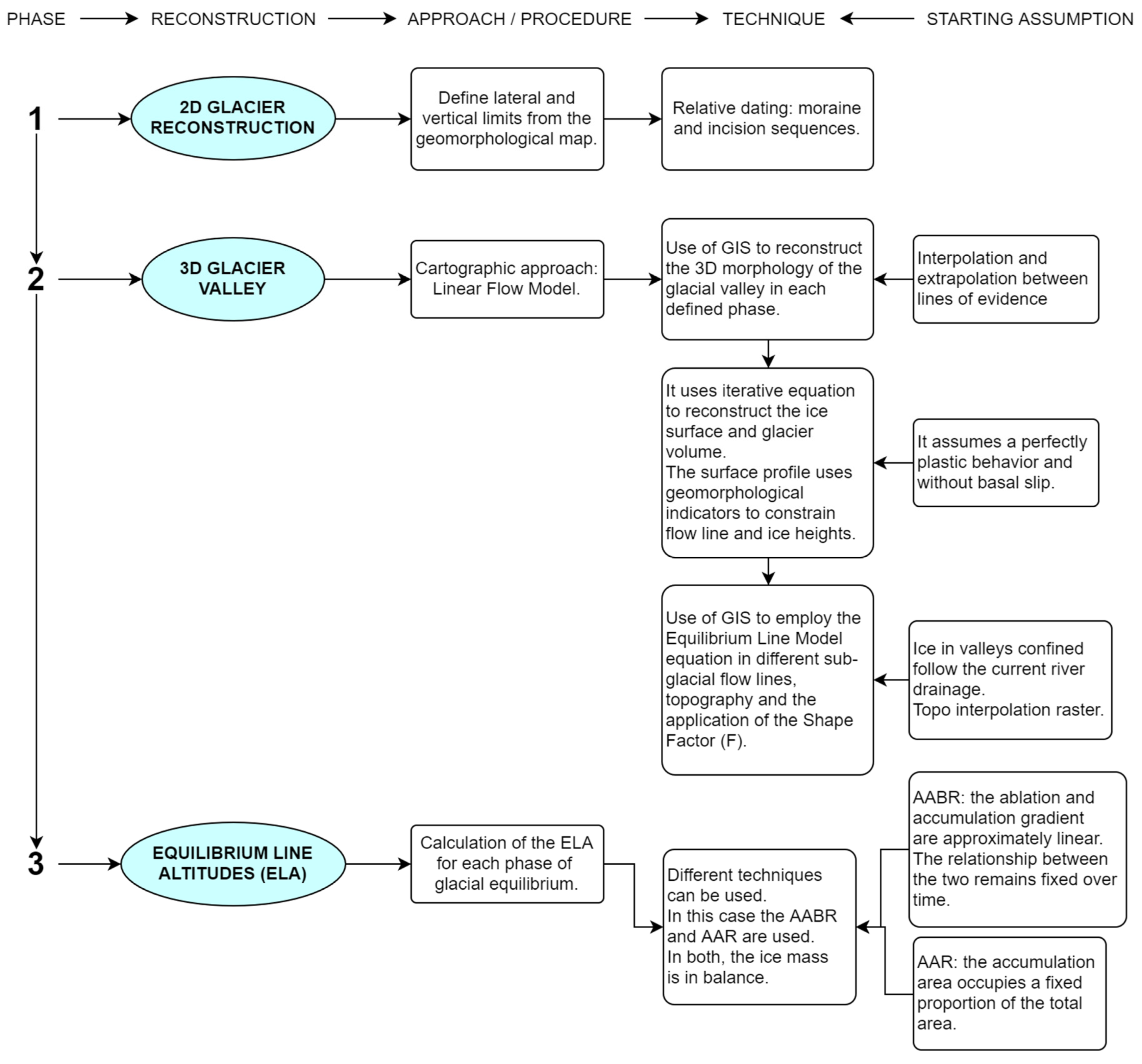
2.2.2. A 3D Reconstruction of the Paleoglacier and PaleoELAs

The steps for obtaining these data are summarized in Figure 5. Firstly, different glacial phases must be delineated. This primarily involves geomorphological criteria. Valley glaciers, such as Peña Negra, are constrained by the surrounding topography, allowing for the identification of structures that demarcate each evolutionary stage (phase). In the headwall area, the main cirque scarp and secondary scarps will indicate different glacier advance stages. On the lateral margins, the maximum height of moraines will serve as evidence of how far the glacial ice extended. Finally, in more distant areas, the maximum heights of frontal moraines will be utilized. All these criteria are conditioned by the evolution of the terrain in the study area.
To calculate the ice volume of the paleoglacier at Peña Negra, the “ArcGIS 10.8” software and the “PalaeoIce” tool [34] are used. This tool provides an automatic method for paleoglacier reconstruction and is based on a review and improvement of the “GlaRe” models [35] and “VOLTA” [36].
“PalaeoIce” utilizes the flowline model, which generates an equilibrium profile along the ice surface following the flowline of a glacier [37,38]. It assumes a perfectly plastic rheological behavior of the ice mass [39,40]. The ice thickness points obtained along the profile will be subsequently used to interpret the three-dimensional distribution of ice thickness and surface elevation of the glacial ice.
To obtain the final result, various morphological and numerical parameters must be entered into the tool. Morphological parameters include the perimeter of the glacier to be modeled (Peña Negra in this case), the corresponding Digital Terrain Model (DTM), and the flow network, which has been manually digitized. Numerical parameters include the point resolution of ice thickness along the flowline (in meters) and the basal shear stress, along with its range of minimum and maximum values (in Pascals). For valley glaciers, the range of values should be between 50 and 150 kPa [38], while for cirque glaciers, it should be higher than 190 kPa [41]. In this case, an intermediate value of 100,000 Pa was used for the basal shear stress, with an upper limit of 150,000 Pa and a lower limit of 50,000 Pa. A specific value for the shape factor (F) is not required, as the tool optimizes this value based on the glacier’s morphology [34]. The calculations are performed using the polynomial fit of [42].
The result will be a Digital Elevation Model (DEM) with ice thickness values within the glacier’s perimeter, created through a Topo to Raster point interpolation process.
Once the total ice thickness is obtained, it is possible to calculate the position of the glacial equilibrium line altitude (ELA). For this, a GIS tool will be used for the automatic calculation of ELAs [43]. To arrive at the ELA value, the Area–Accumulation Ratio (AAR) technique [44] and the Area–Altitude Equilibrium Ratio (AAER) [20] will be used. The Equilibrium Ratio (ER) value used is 1.50, which is the regional estimate [15]. This value is quite close to 1.56, which is the global mean value [44]. For calculating ELA using the AAR method, a value of 0.58 corresponding to the global mean [45] will be used.

2.2.3. Paleoenvironment Calculation (Paleotemperatures and Paleoprecipitation)

Once the ELA elevations data are available, the aim is to estimate the paleoclimatic conditions at this position. The empirical relationship between precipitation and temperature at the ELA is determined through calculations on numerous present-day glaciers [46,47]. This relationship is established when the function of precipitation and temperature is zero, which is the case at the ELA position, using the following equation (Equation (1)) [47]:
P = 5.87 T2 + 230 T + 966
Here, P represents the annual precipitation (mm/year), and T reflects the average temperatures of the summer months (June, July, and August). Summer temperatures are considered, as it is during these months that ice melting is most significant [47]. However, the issue with this equation is that it requires knowing one of the two values during the glacial phase in advance. One possible approach to obtain the average summer temperature is to assume that the dynamics of annual precipitation remain approximately the same. In this case, the variation in ELA would be fully influenced by temperature changes. The most accurate way to calculate the data is by using paleoclimatic indicators. In this study, data from the Navamuño sounding (Béjar) [17] and the sedimentary record of Maltravieso Cave (Cáceres) [48] are utilized (Table 1).
To convert paleotemperature data to their corresponding values at the ELA, the altitudinal gradient value is needed. Since it is not possible to know this value during the glacial period, it will be assumed that the gradient in the area has remained unchanged. The gradient calculation is carried out using the mean temperature values from 11 stations near the area obtained from the Spanish Ministry of the Environment website (https://sig.mapama.gob.es/siga/, accessed on 1 December 2023) (Figure 6). We have obtained for this area an altitudinal gradient value of –0.0066 °C/m. To calculate paleoprecipitation, the value of average summer temperatures must be input. Therefore, the results presented as annual mean values need to be transformed [24,25,49]. It is observed that the values of seasonality, annual mean air temperature, and mean summer temperature are related in the study area.

3. Results

3.1. Characterization of the Different Glacial Phases Recognizable in Peña Negra

In Peña Negra, a total of three main phases are recognizable (Figure 7). Each main phase is delimited by the geomorphological evidence found in the area, as indicated in the first paragraph of Section 2.2.2. Phase 1 marks the state of maximum glacial advance. It occupies the entire glacial valley, and at its head, it is connected to the main cirque scarp. Phase 2 and Phase 3 are stages of lesser magnitude in terms of glacial development. Both phases are delimited at their head by the scarp, the elevation of which closely approximates the height of the moraines. Phase 2 extends to the lateral moraine train located around the middle of the valley. At this point, there is a break in slope in the glacial valley bed, marking the boundary of a stabilization phase [39]. Finally, the smallest phase, Phase 3, can be well delimited by following the maximum height of the upper frontal moraine.

3.2. Results of Ice Volume Calculations

Once the different main and representative phases of the glacier system have been defined, the goal is to calculate the volume of glacial ice. To do this, each phase is individually modeled, following the steps, and using the values presented in Section 2.2.2. Two Digital Elevation Models (DEMs) are obtained for each phase, one representing the thickness of the ice and the other showing the hypsometry of the glacier in equilibrium state (Figure 8). The results for each glacial phase are presented in the following table (Table 2).
It is observed that both the extent and volume decrease as the phases progress. The percentage change in ice volume from Phase 1 to Phase 2 is 71.1%, while the change in the area covered by ice is 38.89%. The relationship between Phase 2 and Phase 3 indicates a decrease of 86.85% in ice volume and a 65.45% reduction in the area covered.

3.3. Value and Variation in the Position of the ELAs

For each glacial phase, a total of two Equilibrium line altitudes (ELAs) are obtained (Figure 8B,D,F), each using a different method: AAR [44] or AABR [20] (Table 3). The steps and values used to obtain them are described in Section 2.2.2. In the case of Phase 1, it is assumed that the precipitation regime was at least like that of Phase 2, as there were no paleoclimatic data found that were sufficiently close to the study area during its evolutionary development.
To make a comparison with current conditions, it is necessary to know the theoretical position of the ELA and the climatic values from thermometric stations. Current annual average precipitation data are taken from the La Covatilla thermopluviometric station (Béjar), which is located less than 1 km from the study area. Using the current average precipitation values (information compiled by the State Meteorological Agency, AEMET), a theoretical current ELA value for Peña Negra of 2612.94 m is obtained. The comparison with the values obtained for the paleoELAs is shown in Table 4.
It is important to note that the results are subject to an uncertainty error that accumulates with progress in the calculation processes: (1) the position of the ELA is influenced by the initial reconstruction of the paleoglacier, which assumes uncertain bed conditions [35,40,42]; (2) the value of the altitudinal gradient; (3) the standard deviation of the relationship between mean summer temperatures and precipitation (±750 mm) [46,47]; (4) the value of each paleoclimatic data point [48].

4. Discussion

4.1. Meaning of the Geomorphological Features Described in Peña Negra

The geomorphological record reveals four clearly distinguished sequences of deposits (Phases 1, 2, 3, and the late phase moraine), separated by a basal moraine and obstruction deposits or peat bogs. Within these sequences, both Phases 2 and 3 exhibit approximately five episodes of incision/overlay that allow the determination of the relative chronological order of ice advance/retreat phases. Each set of moraines indicates rapid changes in the glacier’s dynamics, demonstrating that Peña Negra responds quickly to paleoclimatic variations. One hypothesis to explain this high sensitivity to climatic variations is the limited size of the glacier’s accumulation area [13]. Consequently, during periods of negative mass balance, the ice accumulated in the head areas could not compensate for the losses due to summer melting. However, under optimal conditions for a positive mass balance, the glacier could recover more easily.
Other intrinsic factors of the paleoglacier, such as its topographical position and orientation, significantly influenced its development. Through geomorphological evidence preserved in its erosional and depositional forms, a relative age of its origin can be determined. The topographical location of the main cirque scarp of Peña Negra, embedded in other nearby paleoglaciers (such as El Oso or El Trampal) and linked to that of El Endrinal, indicates that its development was the most recent. This implies a longer time for the attainment of optimal paleoclimatic conditions to host a stable ice body. Similarly, it was the first to be affected by unfavorable paleoclimatic variations when it was in equilibrium (mass balance equal to 0). Moreover, the smaller number of moraine sequences compared to other paleoglaciers in the massif marks a genesis of the paleoglacier subsequent to the other paleoglaciers.
As a result of these factors, Peña Negra would have housed ice for a shorter period and would have had a smaller thickness. Both factors could explain the limited variety and size of its erosional features.

4.2. Evolutionary and Chronological Stages of Peña Negra

Four main stages can be distinguished in the evolution of Peña Negra. Phase 1, the oldest in chronological terms, depicts a valley glacier with the maximum ice advance. Next is Phase 2, which features the first sequence of overlapping lateral moraines. Finally, we reach a terminal stage of the glacier where the transition from a valley glacier to a cirque glacier is evident (Figure 9A,B). In this latter period, Phase 3, frontal moraines in a semilunar shape are recorded, indicating the position of the small glacial front. Phase 4 is represented by small moraines at the base of the cirque.
The main phases defined in the paleoglacier of Peña Negra can be correlated with the evolutionary models proposed for the Sierra de Béjar-Candelario during the Last Glacial Maximum (Late Pleistocene). These models outline an initial ice cap phase, followed by three evolutionary phases confined to the valleys [13,15,16,49]. This evolutionary trend is also observed in the Central Iberian System. The model suggests that the phase of maximum ice extent in the Central Iberian System follows an asynchronous pattern, indicating it was not synchronous in all paleoglaciers, unlike the later phases that conform to more consistent timeframes [4,5,6,23,50].
Geomorphological evidence shows that Peña Negra reached its maximum ice extent relatively late [13]. This suggests that this phase was likely after the maximum ice extent phase dated at approximately 25.0 ± 1.5 ka in the Cuerpo de Hombre paleoglacier [16] or at 25.0 ± 1.4 ka in paleoglaciers of the Sierra de Gredos [23]. Phase 1 of Peña Negra should be placed within a later phase, which is constrained between 25 and 21 ka and experienced various oscillations (advance/retreat) [4,5,6,23,50]. This maximum extent phase would fall within the Last Glacial Maximum [51].
Phase 2 represents an evolutionary stage of reduced ice extent, marked by a sequence with several pulsations denoting a trend of ice loss. This deglaciation stage, with several minor periods of ice front fluctuations, is framed around 19–17 ka [23,50].
Finally, Peña Negra becomes limited to a cirque glacier (Figure 8B). This terminal phase would be around 15–13 ka, during which the final sequence of frontal moraines is deposited. The deposit occurred during stable phases as the ice retreated. The topographic and hypsometric characteristics of Peña Negra signal the conclusion of the glacier system’s development after this phase. Other paleoglaciers with greater extent, cirque size, and ice volume may have left later records of glacial activity until the glacier system finally ceased to function at the beginning of the Holocene [23,50]. In this glacier, this last phase (phase 4) could correspond to the moraines at the base of the cirque and to the last glacial advance during the Younger Dryas.

4.3. Paleoenvironmental Reconstruction of Peña Negra

The data obtained from the precipitation and temperature balance formula at the Equilibrium line altitude (ELA), in line with the evolution proposed for Peña Negra in this study, indicate a progressive decrease in paleotemperatures and paleoprecipitation (Table 4). This directly influenced a predominantly negative mass balance, promoting the gradual retreat of the ice. The reduction in ice volume and the retreat of the glacier area coincide with the progressive increase in the topographical position of the ELAs.
When comparing the ELA data from other studies for an evolutionary state of maximum ice extent (equivalent to Phase 1) in the Sierra de Béjar-Candelario [15,16], Peña Negra has the lowest values throughout the massif. Regarding the ELA values for Peña Negra presented in [15], there is a variation of −81.5 m for the AAR method and +25.5 m for the AABR method. The general ELA for the Sierra de Béjar-Candelario was established at 2010 m [15]. This implies that, in comparison to other paleoglaciers, Peña Negra required a higher volume of winter precipitation to achieve a positive mass balance that allowed glacier advance, as its average summer temperatures were higher. Peña Negra was especially sensitive to precipitation variations, responding rapidly with ice advance during wetter periods (positive mass balance) and retreat during phases of reduced precipitation (negative mass balance).
The Heinrich Stadials [52], which occurred during the Last Glacial Cycle (Late Pleistocene), mainly within the last 100 thousand years, recorded paleoclimatic conditions with decreasing temperatures and precipitation. These conditions would have resulted in reduced snowfall, impeding glacier advance and leading to a negative mass balance [53,54,55]. Analysis of the Upper Pleistocene glacier record, often well-preserved, enables the reconstruction of paleoclimatic conditions (precipitation and temperatures) at the time of its formation [1]. Current models based on a large database of exposure to terrestrial cosmogenic nuclides in the Mediterranean area indicate a major accumulation trend of advancing phase dates outside the Heinrich Stadial ranges [55]. The Heinrich Stadials that occurred during this late Late Pleistocene period, with evidence of glacier system development in the region, are HS 3 (32.7–31.3 ka), HS 2 (26.5–24.3 ka), and HS 1 (18.0–15.6 ka) [55,56,57]. The phases of glacial stability in which Peña Negra’s moraines formed correlate more effectively with intervals between Heinrich Stadials than the closer paleoglaciers, especially during the phase of maximum ice expansion. These variations in paleotemperatures and paleoprecipitation are evident not only in the geomorphological record of the glacier system but also in changes in vegetation and human settlements during these colder and drier intervals [54,58].

5. Conclusions

The detailed study of the Peña Negra paleoglacier system has provided valuable insights into its evolution during MIS 2, as well as approximate paleoclimatic conditions (temperature and precipitation). From this research, the following conclusions can be drawn:
  • Due to its hypsometric and topographic characteristics, the Peña Negra paleoglacier system was highly sensitive to climatic variations at the end of the LGC (Late Pleistocene). This sensitivity is evident in the sequences of lateral and frontal moraines, which show small cycles of ice advance and retreat.
  • The evolutionary sequences of the paleoglacier system correlate with the phases described in the evolutionary models of the study area. Specifically, three main phases can be distinguished, demonstrating a gradual retreat in ice extent. The combination of fieldwork with high-resolution data collection techniques provides a better understanding of cirque glacier scarps and terraced walls, resulting in a more precise description of the evolutionary phases.
  • Paleoclimatic data obtained from the equilibrium line altitudes (ELAs) calculated for each phase reveal a clear increase in precipitation and a slight decrease in average summer temperatures compared to current conditions. This suggests that precipitation variations were the primary factors responsible for moments of positive and negative mass balance. The paleoclimatic study of the paleoglaciers closest to Peña Negra will allow for a more comprehensive understanding of the paleoclimatic patterns that occurred during the different phases of stability recorded in the Sierra de Béjar-Candelario.
  • During MIS 2, there were alternating cold and arid periods (Heinrich Stadials) with slightly warmer and wetter periods. The stability phases that led to the formation of moraine records are associated with these last moments in which the mass balance was positive due to the notable increase in precipitation in the form of snow.

Author Contributions

Conceptualization, C.E.N., A.C., R.C., A.M.M.-G., J.L.G. and J.Á.G.-D.; methodology, C.E.N., A.C., R.C., A.M.M.-G., J.L.G. and J.Á.G.-D.; software, C.E.N.; validation, C.E.N., R.C., A.M.M.-G. and J.L.G.; formal analysis, C.E.N., A.C., R.C., A.M.M.-G., J.L.G. and J.Á.G.-D.; investigation, C.E.N. and A.C.; resources, C.E.N., A.C., R.C., A.M.M.-G. and J.L.G.; data curation, C.E.N., A.C., R.C., A.M.M.-G. and J.L.G.; writing—original draft preparation, C.E.N.; writing—review and editing, C.E.N., A.C., R.C., A.M.M.-G., J.L.G. and J.Á.G.-D.; visualization, C.E.N.; supervision, R.C., A.M.M.-G. and J.L.G.; project administration, A.M.M.-G.; funding acquisition, A.M.M.-G. All authors have read and agreed to the published version of the manuscript.

Funding

Grant 131874B-I00 funded by MCIN/AEI/10.13039/501100011033. Ministry for the Ecological Transition and the Demographic Challenge.

Institutional Review Board Statement

Not applicable.

Informed Consent Statement

Not applicable.

Data Availability Statement

The data presented in this study are available within this article.

Acknowledgments

This research was assisted by GEAPAGE research group (Environmental Geomorphology and Geological Heritage) of the University of Salamanca.

Conflicts of Interest

The authors declare no conflict of interest.

References

  1. Hughes, P.D.; Woodward, J.C. Quaternary glaciation in the Mediterranean mountains: A new synthesis. Geol. Soc. Lond. Spec. Publ. 2017, 433, 1–23. [Google Scholar] [CrossRef]
  2. Naughton, F.; Sánchez-Goñi, M.F.; Desprat, S.; Turon, J.L.; Duprat, J.; Malaize, B.; Joli, C.; Cortijo, E.; Drago, T.; Freitas, M.C. Present-day and past (last 25000 years) marine pollen signal off western Iberia. Mar. Micropaleontol. 2007, 62, 91–114. [Google Scholar] [CrossRef]
  3. Hogg, A.; Southon, J.; Turney, C.; Palmer, J.; Bronk Ramsey, C.; Fenwick, P.; Boswijk, G.; Friedrich, M.; Helle, G.; Hughen, K.; et al. Punctuated shutdown of Atlantic meridional overturning circulation during Greenland Stadial 1. Sci. Rep. 2016, 6, 25902. [Google Scholar] [CrossRef] [PubMed]
  4. Palacios, D.; de Andrés, N.; de Marcos, J.; Vázquez-Selem, L. Glacial landforms and their paleoclimatic significance in Sierra de Guadarrama, Central Iberian Peninsula. Geomorphology 2012, 139, 67–78. [Google Scholar] [CrossRef]
  5. Palacios, D.; Andrés, N.; Marcos, J.; Vázquez-Selem, L. Maximum glacial advance and deglaciation of the Pinar Valley (Sierra de Gredos, Central Spain) and its significance in the Mediterranean context. Geomorphology 2012, 177, 51–61. [Google Scholar] [CrossRef]
  6. Palacios, D.; Andrés, N.; Vieira, G.; Marcos, J.; Vázquez-Selem, L. Last Glacial Maximum and deglaciation of the Iberian Central System. In Proceedings of the EGU General Assembly Conference Abstracts, Vienna, Austria, 22–27 April 2012; p. 3738. [Google Scholar]
  7. Pedraza, J.; Carrasco, R.M.; Domínguez-Villar, D.; Villa, J. Late Pleistocene glacial evolutionary stages in the Gredos mountains (Iberian Central System). Quat. Int. 2013, 302, 88–100. [Google Scholar] [CrossRef]
  8. Prado, C. Descripción Física y Geológica de la provincia de Madrid; Colegio de Ingenieros de Caminos Canales y Puertos de Madrid (reedición de 1975): Madrid, Spain, 1864; 325p. [Google Scholar]
  9. Baysselance, E. Quelques traces glaciaires en Espagne. Annu. Club Alp. Française 1884, 10, 410–416. [Google Scholar]
  10. Schmieder, O. Die Sierra de Gredos. Mitteilungen der Geographischen Gesellschaft in Manchen. Estud. Geográficos 1953, 14, 629. [Google Scholar]
  11. Obermaier, H.; Carandell, J. Nuevos datos para la extensión del glaciarismo cuaternario en la Cordillera Central. Bol. Real Soc. Esp. Hist. Nat. 1916, XVII, 252–260. [Google Scholar]
  12. Carrasco, R.M.; Pedraza, J.; Domínguez-Villar, D.; Muñoz-Rojas, J. El glaciarismo Pleistoceno de la Sierra de Béjar (Gredos occidental, Salamanca, España): Nuevos datos para precisar su extensión y evolución). Bol. R. Soc. Esp. Hist. Nat. Sec. Geol. 2008, 102, 35–45. [Google Scholar]
  13. Cruz, R.; Goy, J.L.; Zazo, C. Las sierras de Béjar y del Barco durante el Cuaternario, Glaciarismo y Periglaciarismo: Libro guía; Sección de Publicaciones de la Escuela Técnica Superior de Ingenieros Industriales, Universidad Politécnica de Madrid: Madrid, Spain, 2007. [Google Scholar]
  14. Carrasco, R.M.; Villa, J.; Pedraza, J.D.; Dominguez-Villar, D.; Willenbring, J.K. Reconstruction and chronology of the Sierra de Bejar plateau glacier (Spanish Central System) during the glacial maximum. Boletín Real Soc. Española Hist. Nat. Sección Geológica 2011, 105, 125–135. [Google Scholar]
  15. Carrasco, R.M.; Pedraza, J.; Domínguez-Villar, D.; Villa, J.; Willenbring, J.K. The plateau glacier in the Sierra de Béjar (Iberian Central System) during its maximum extent. Reconstruction and chronology. Geomorphology 2013, 196, 83–93. [Google Scholar] [CrossRef]
  16. Carrasco, R.M.; Pedraza, J.; Domínguez-Villar, D.; Willenbring, J.K.; Villa, J. Sequence and chronology of the Cuerpo de Hombre paleoglacier (Iberian Central System) during the last glacial cycle. Quat. Sci. Rev. 2015, 129, 163–177. [Google Scholar] [CrossRef]
  17. López-Sáez, J.A.; Carrasco, R.M.; Turu, V.; Ruiz-Zapata, B.; Gil-García, M.J.; Luelmo-Lautenschlaeger, R.; Pérez-Díaz, S.; Alba-Sánchez, F.; Abel-Schaad, D.; Ros, X.; et al. Late Glacial-early holocene vegetation and environmental changes in the western Iberian Central System inferred from a key site: The Navamuño record, Béjar range (Spain). Quat. Sci. Rev. 2020, 230, 106167. [Google Scholar] [CrossRef]
  18. Chazarra, A.; Flórez-García, E.; Peraza-Sánchez, B.; Tohá-Rebull, T.; Lorenzo-Mariño, B.; Criado, E.; Moreno-García, J.V.; Romero-Fresneda, R.; Botey, M.R. Mapas Climáticos de España (1981–2010) y Eto (1996–2016); Agencia Estatal de Meteorología (AEMET): Madrid, Spain, 2018. [Google Scholar]
  19. Santa Regina, I. Estimaciones de la Radiación Solar Según la Topografía Salmantina; Ediciones de la Diputación: Madrid, Spain, 1987; p. 154. [Google Scholar]
  20. Osmaston, H. Estimates of glacier equilibrium line altitudes by the Area × Altitude, the Area×Altitude Balance Ratio and the Area×Altitude Balance Index methods and their validation. Quat. Int. 2005, 138–139, 22–31. [Google Scholar] [CrossRef]
  21. Vieira, G. Combined numerical and geomorphological reconstruction of the Serra da Estrela plateau icefield, Portugal. Geomorphology 2008, 97, 190–207. [Google Scholar] [CrossRef]
  22. Palacios, D.; Andrés, N.; Úbeda, J.; Alcalá, J.; Marcos, J.; Vázquez-Selem, L. The importance of poligenic moraines in the paleoclimatic interpretation from cosmogenic dating. In Proceedings of the EGU General Assembly Conference Abstracts, Vienna, Austria, 22–27 April 2012; p. 3759. [Google Scholar]
  23. Carrasco, R.M.; Turu, V.; Soteres, R.L.; Fernández-Lozano, J.; Karampaglidis, T.; Rodés, Á.; Ros, X.; Andrés, N.; Granja-Bruña, J.L.; Muñoz-Martín, A.; et al. The Prados del Cervunal morainic complex: Evidence of a MIS 2 glaciation in the Iberian Central System synchronous to the global LGM. Quat. Sci. Rev. 2023, 312, 108169. [Google Scholar] [CrossRef]
  24. Pellitero, R. Evolución finicuaternaria del glaciarismo en el macizo de Fuentes Carrionas (Cordillera Cantábrica), propuesta cronológica y paleoambiental. Cuaternario Geomorfol. 2013, 27, 71–90. [Google Scholar]
  25. Pellitero, R.; Fernández-Fernández, J.M.; Campos, N.; Serrano, E.; Pisabarro, A. Late Pleistocene climate of the northern Iberian Peninsula: New insights from palaeoglaciers at Fuentes Carrionas (Cantabrian Mountains). J. Quat. Sci. 2019, 34, 342–354. [Google Scholar] [CrossRef]
  26. Rettig, L.; Monegato, G.; Spagnolo, M.; Hajdas, I.; Mozzi, P. The Equilibrium line altitude of isolated glaciers during the Last Glacial Maximum—New insights from the geomorphological record of the Monte Cavallo Group (south-eastern European Alps). CATENA 2023, 229, 107187. [Google Scholar] [CrossRef]
  27. Bellido, F. Mapa Geológico de Béjar, 1:50 000. Map 553; Instituto Geológico y Minero de España: Madrid, Spain, 2004. [Google Scholar]
  28. De Vicente, G.; Cunha, P.P.; Muñoz-Martín, A.; Cloetingh, S.A.P.L.; Olaiz, A.; Vegas, R. The Spanish-Portuguese Central System: An example of intense intraplate deformation and strain partitioning. Tectonics 2018, 37, 4444–4469. [Google Scholar] [CrossRef]
  29. Cruz, R. Análisis Geológico Ambiental del Espacio Natural de Gredos. Cartografía del Paisaje e Itinerarios Geoambientales. Tratamiento y Representación Mediante SIG. Doctoral Dissertation, Universidad de Salamanca, Salamanca, Spain, 2006. [Google Scholar]
  30. Cruz, R.; Goy, J.L.; Zazo, C. El registro periglaciar en la Sierra del Barco (Sistema Central) y su relación con el sistema glaciar pleistoceno. Finisterra 2009, 44, 9–22. [Google Scholar]
  31. Cruz, R.; Goy, J.L.; Zazo, C. Hydrological Patrimony in the mountainous areas of Spain: Geodiversity inventory and cataloguing of the Sierras De Béjar and Del Barco (in the Sierra de Gredos of the Central System). Environ. Earth Sci. 2014, 71, 85–97. [Google Scholar] [CrossRef]
  32. Martínez-Graña, A.M.; Goy, J.L.; González-Delgado, J.A.; Cruz, R.; Sanz, J.; Cimarra, C.; De Bustamante, I. 3D virtual itinerary in the geological heritage from natural areas in Salamanca-Ávila-Cáceres, Spain. Sustainability 2018, 11, 144. [Google Scholar] [CrossRef]
  33. Carrasco, R.M. Geomorfología del Valle del Jerte. Las Líneas Maestras del Paisaje. Doctoral Dissertation, Universidad de Extremadura (UEX), Cáceres, Spain, 1999. [Google Scholar]
  34. Li, Y. PalaeoIce: An automated method to reconstruct palaeoglaciers using geomorphic evidence and digital elevation models. Geomorphology 2023, 421, 108523. [Google Scholar] [CrossRef]
  35. Pellitero, R.; Rea, B.R.; Spagnolo, M.; Bakke, J.; Ivy-Ochs, S.; Frew, C.R.; Hughes, P.; Ribolini, A.; Lukas, S.; Renssen, H. GlaRe, a GIS tool to reconstruct the 3D surface of palaeoglaciers. Comput. Geosci. 2016, 94, 77–85. [Google Scholar] [CrossRef]
  36. James, W.H.M.; Carrivick, J.L. Automated modelling of spatially-distributed glacier ice thickness and volume. Comput. Geosci. 2016, 92, 90–103. [Google Scholar] [CrossRef]
  37. Nye, J.F. The Mechanics of Glacier Flow. J. Glaciol. 1952, 2, 82–93. [Google Scholar] [CrossRef]
  38. Nye, J.F. A method of calculating the thicknesses of the ice-sheets. Nature 1952, 169, 529–530. [Google Scholar] [CrossRef]
  39. Paterson, W.S.B. Physics of Glaciers; Butterworth-Heinemann: Oxford, UK, 2000. [Google Scholar]
  40. Benn, D.I.; Hulton, N.R.J. An ExcelTM spreadsheet program for reconstructing the surface profile of former mountain glaciers and ice caps. Comput. Geosci. 2010, 36, 605–610. [Google Scholar] [CrossRef]
  41. Weertman, J. Shear Stress at the Base of a Rigidly Rotating Cirque Glacier. J. Glaciol. 1971, 10, 31–37. [Google Scholar] [CrossRef]
  42. Li, H.; Ng, F.; Li, Z.; Qin, D.; Cheng, G. An extended “perfect-plasticity” method for estimating ice thickness along the flow line of mountain glaciers. J. Geophys. Res. Earth Surf. 2012, 117, 76–95. [Google Scholar] [CrossRef]
  43. Pellitero, R.; Rea, B.R.; Spagnolo, M.; Bakke, J.; Hughes, P.; Ivy-Ochs, S.; Lukas, S.; Ribolini, A. A GIS tool for automatic calculation of glacier equilibrium-line altitudes. Comput. Geosci. 2015, 82, 55–62. [Google Scholar] [CrossRef]
  44. Serrano-Cañadas, E.; González-Trueba, J.J. El método AAR para la determinación de paleo-ELAs: Análisis metodológico y aplicación en el Macizo de Valdecebollas (Cordillera Cantábrica). Cuad. Investig. Geográfica 2004, 30, 7–34. [Google Scholar] [CrossRef]
  45. Oien, R.P.; Rea, B.R.; Spagnolo, M.; Barr, I.D.; Bingham, R.G. Testing the area–altitude balance ratio (AABR) and accumulation–area ratio (AAR) methods of calculating glacier equilibrium-line altitudes. J. Glaciol. 2022, 68, 357–368. [Google Scholar] [CrossRef]
  46. Ohmura, A.; Kasser, P.; Funk, M. Climate at the Equilibrium Line of Glaciers. J. Glaciol. 1992, 38, 397–411. [Google Scholar] [CrossRef]
  47. Ohmura, A.; Boettcher, M. Climate on the equilibrium line altitudes of glaciers: Theoretical background behind Ahlmann’s P/T diagram. J. Glaciol. 2018, 64, 489–505. [Google Scholar] [CrossRef]
  48. Bañuls Cardona, S.; López-García, J.M.; Blain, H.-A.; Canals Salomó, A. Climate and landscape during the Last Glacial Maximum in southwestern Iberia: The small-vertebrate association from the Sala de las Chimeneas, Maltravieso, Extremadura. Comptes Rendus Palevol 2012, 11, 31–40. [Google Scholar] [CrossRef]
  49. Pedraza, J.D.; Carrasco, R.M. El glaciarismo pleistoceno del Sistema Central. Enseñanza Cienc. Tierra 2005, 13, 278–288. [Google Scholar]
  50. Oliva, M.; Palacios, D.; Fernández-Fernández, J.M.; Rodríguez-Rodríguez, L.; García-Ruiz, J.M.; Andrés, N.; Carrasco, R.M.; Pedraza, J.D.; Pérez-Alberti, A.; Valcárcel, M.; et al. Late Quaternary glacial phases in the Iberian Peninsula. Earth-Sci. Rev. 2019, 192, 564–600. [Google Scholar] [CrossRef]
  51. Clark, P.U.; Dyke, A.S.; Shakun, J.D.; Carlson, A.E.; Clark, J.; Wohlfarth, B.; Mitrovica, J.X.; Hostetler, S.W.; McCabe, A.M. The Last Glacial Maximum. Science 2009, 325, 710–714. [Google Scholar] [CrossRef] [PubMed]
  52. Heinrich, H. Origin and Consequences of Cyclic Ice Rafting in the Northeast Atlantic Ocean During the Past 130,000 Years. Quat. Res. 1988, 29, 142–152. [Google Scholar] [CrossRef]
  53. Hughes, P.D.; Woodward, J.; Gibbard, P.L. Late Pleistocene glaciers and climate in the Mediterranean. Glob. Planet. Change 2006, 50, 83–98. [Google Scholar] [CrossRef]
  54. Ludwig, P.; Shao, Y.; Kehl, M.; Weniger, G.C. The Last Glacial Maximum and Heinrich event I on the Iberian Peninsula: A regional climate modelling study for understanding human settlement patterns. Glob. Planet. Change 2018, 170, 34–47. [Google Scholar] [CrossRef]
  55. Allard, J.L.; Hughes, P.D.; Woodward, J.C. Heinrich Stadial aridity forced Mediterranean-wide glacier retreat in the last cold stage. Nat. Geosci. 2021, 14, 197–205. [Google Scholar] [CrossRef]
  56. Sánchez-Goñi, M.F.; Harrison, S.P. Millennial-scale climate variability and vegetation changes during the Last Glacial: Concepts and terminology. Quat. Sci. Rev. 2010, 29, 2823–2827. [Google Scholar] [CrossRef]
  57. Seierstad, I.K.; Abbott, P.M.; Bigler, M.; Blunier, T.; Bourne, A.J.; Brook, E.; Buchardt, S.L.; Buizert, C.; Clausen, H.B.; Cook, E.; et al. Consistently dated records from the Greenland GRIP, GISP2 and NGRIP ice cores for the past 104 ka reveal regional millennial-scale δ18O gradients with possible Heinrich event imprint. Quat. Sci. Rev. 2014, 106, 29–46. [Google Scholar] [CrossRef]
  58. Fletcher, W.J.; Goni, M.F.S.; Allen, J.R.; Cheddadi, R.; Combourieu-Nebout, N.; Huntley, B.; Lawson, I.; Londeix, L.; Magri, D.; Margari, V.; et al. Millennial-scale variability during the last glacial in vegetation records from Europe. Quat. Sci. Rev. 2010, 29, 2839–2864. [Google Scholar] [CrossRef]
Figure 1. Location map of the study area. In the pink mark is the Peña Negra paleoglacier.
Sustainability 15 16514 g001
Figure 2. Geological map of Peña Negra.
Sustainability 15 16514 g002
Figure 3. Geomorphological map of Peña Negra.
Sustainability 15 16514 g003
Figure 4. Bird’s-eye view photographs from the western area of the Peña Negra cirque. (A) Complexes of lateral and frontal moraines. (B) Complex of frontal moraines and complex of lateral moraines of the E slope of the glacial valley. (C) Lateral surface of the cirque covered by periglacial cones. (D) Polished surfaces belonging to the minority erosional forms in this paleoglacier. (E) Panoramic of the Peña Negra paleoglacier cirque. The upper limit of the cirque is marked.
Sustainability 15 16514 g004
Figure 5. Methodological scheme of Section 2.2.2.
Sustainability 15 16514 g005
Figure 6. Location of the climatological stations and relationship of the altitudinal gradient.
Sustainability 15 16514 g006
Figure 7. Area of the different main phases of Peña Negra.
Sustainability 15 16514 g007
Figure 8. Ice volume thickness and hypsometry for each main phase of Peña Negra. The value of the calculated ELAs is represented. (A) Ice thickness in Phase 1. (B) Hypsometries and ELAs in Phase 1. (C) Ice thickness in Phase 2. (D) Hypsometries and ELAs in Phase 2. (E) Ice thickness in Phase 3. (F) Hypsometries and ELAs in Phase 3.
Sustainability 15 16514 g008
Figure 9. (A) A 3D reconstruction of the Peña Negra cirque. (B) Reconstruction of the Peña Negra glacier during the cirque phase (Phase 3).
Sustainability 15 16514 g009
Table 1. Paleotemperature data.
Tª (°C)Altitude (m)Age (cal. BP)SiteSource
112.4 ± 1.5 (MTW)44419,500–18,700Cáceres[48]
26.25 (MAAT)150515,090Navamuño[17]
ª Abbreviations for temperature data correspond to: Mean Temperature of the Warmest Month (MTW) and Mean Annual Air Temperature (MAAT).
Table 2. Dimensional data and position of the paleoELA for the different phases of Peña Negra.
PhaseTotal Ice Volume (km3)3D Extension (ha)paleoELA AAR (m)paleoELA AABR (m)
Phase 1 0.526195.161861.51836.5
Phase 20.152119.281934.51909.5
Phase 30.02041.581963.21938.5
The represented ELAs were calculated from the Digital Elevation Model (DEM) obtained through the polynomial adjustment of [42].
Table 3. Variation in the position of ELA with respect to current theoretical ELA.
Phase paleoELA AAR (m)ΔELA AAR (m)paleoELA AABR (m)ΔELA AABR (m)
Phase 11861.5−776.441836.5−751.44
Phase 21934.5−678.441909.5−703.44
Phase 31963.2−649.741938.5−674.94
The calculation of ΔELA (m) is carried out by comparing the values of the paleoELAs with the value of the current ELA: 2612.94 m.
Table 4. Climatological variations with respect to current values.
Phase ΔT (°C) AARΔT (°C) AABRΔP (mm) AARΔP (mm) AAR
Phase 1−2.96−2.56+1281.87 ± 750+1335.64 ± 750
Phase 2−2.12−2.15+1281.87 ± 750+1335.64 ± 750
Phase 3−1.18−0.78+1529.85 ± 750+1595.25 ± 750
It is assumed that the precipitation values in Phase 1 were at least like Phase 2. The comparison is made with respect to the average value of precipitation and the average values of summer temperatures measured today in the ELA.
Disclaimer/Publisher’s Note: The statements, opinions and data contained in all publications are solely those of the individual author(s) and contributor(s) and not of MDPI and/or the editor(s). MDPI and/or the editor(s) disclaim responsibility for any injury to people or property resulting from any ideas, methods, instructions or products referred to in the content.

