

Construction and Change Analysis of Water Ecosystem Service Flow Networks in the Xiangjiang River Basin (XRB)
College of Resource and Environment Sciences, Hunan Normal University, Changsha 410081, China
*
Author to whom correspondence should be addressed.
†
These authors contributed equally to this work.
Sustainability 2024, 16(9), 3813; https://doi.org/10.3390/su16093813
Submission received: 2 April 2024
/
Revised: 24 April 2024
/
Accepted: 29 April 2024
/
Published: 1 May 2024
(This article belongs to the Topic Hydrology and Water Resources Management)
Abstract
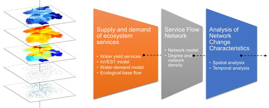
:Clearing and successfully characterizing ecosystem service flow paths has become a key bottleneck restricting in-depth research on the supply and demand relationships of ecosystem services. At present, although some explorations have been performed using water ecosystem services as a pioneer, the nature of its network and the fact that ecological base flow needs to be eliminated have been ignored. This study used InVEST and network models to consider ecological base flow, quantifying the supply, demand, and flow paths of freshwater ecosystem services in the Xiangjiang River Basin. The results showed that the overall distribution of the water supply in the Xiangjiang River Basin from 2000 to 2020 shows a pattern of higher supply in the south and lower supply in the north. The distribution of water demand shows higher levels in the north and lower levels in the south. The network density remains at its maximum level. The results of this study have provided a scientific basis for water resource management in river basins and improving ecological compensation mechanisms.
1. Introduction
The concept of ecosystem services refers to the benefits that individuals gain from their environment. They are often referred to as bridges between natural and social systems [1,2,3]. With the continuous expansion and intensification of human disturbance, the structure and pattern of ecosystems have undergone major changes. This has accelerated the degradation of ecosystem functions, threatening the ecological security and sustainability of human society [4]. This is because of the mismatch and imbalance caused by the combined effects of socioeconomic and natural factors on ES supply and demand [5,6,7]. Therefore, ecosystem services cannot be assessed and regulated solely from the perspectives of static supply and demand. A dynamic description of the flow channel and network of ecosystem services is also required to compensate for the lack of understanding of the mechanism and path of the flow and the flow direction of ecosystem service supply and demand [8,9,10]. This offers a more grounded scientific foundation for the development of ecosystem service-based ecological optimization policies.
Ecosystem service flow (ESF) is an extension of ecosystem service supply and demand. Early research focused primarily on the supply perspective [11]. The connection between ecosystem services and human well-being is more closely aligned with its essential bridging characteristics when considering ecosystem services from the supply and demand standpoint [12]. The ecosystem service flows generated by complex ES spatial flows complement the characteristics of ecosystem services, that is, the volume of flow, flow direction, and flow path from the supply area to the demand area [13]. The advantage of this concept is its ability to distinguish between the potential supply (demand) and actual supply (demand) of ecosystem services [14]. This is mainly because, in the actual ES flow process, there are certain “sinks” in the connection area between the supply area and the demand area. This can consume or hinder the flow of ecosystem services, resulting in not all potential supply being able to be converted into actual supply [15].
The study of ecosystem service flows remains in the early stages of development. However, there is still no unified definition of the concept and no fully developed theoretical framework. However, to date, easy-to-operate quantitative methods and system models have been lacking [8,16,17]. Given their inherent mobility and through detailed evaluation, freshwater ecosystem services have drawn the greatest attention in recent research on ecosystem service flows [18,19]. In general, this includes two perspectives, that is, terrain and runoff. Li, et al. [20] combined a digital elevation model with a supply and consumption matrix to quantify two different water supply service flows at the grid and administrative scales in the Beijing–Tianjin–Hebei region of China. Meanwhile, Zhang, et al. [21] considered the two runoff generation mechanisms of excess infiltration and infiltration saturation and quantified the freshwater service supply in the Weihe River Basin in China using the VIC model. However, characterizing ESF flow paths remains a challenge. To date, some researchers have examined the relationship between ESF and ES in distribution from production to consumption. However, the flow path has not yet been determined because of the insufficient consideration of the ecosystem status and structure [22]. In the context of the ecosystem structure, it comprises an interactive network superimposed on social and economic activities. Some researchers have confirmed the application potential of network models based on freshwater ESF [23,24]. Nodes represent specific objects such as people and species or areas. Edges represent physical relationships such as predation and supply or social relationships such as interpersonal relationships between the elements in the network model. This approach is similar to the mechanisms of ESF. Chen, Lin, and Huang [19] found that linking ecosystem service flows with ecological security patterns could identify vulnerable nodes in a region that may pose threats to water security. However, in the process of measuring freshwater ecosystem services, the minimum amount of water required to preserve the fundamental form and basic ecological functions of the river is not retained. This is an ecological baseflow. This needs to be eliminated from an ecological sustainability perspective [25,26].
In summary, the main objectives of this study were to quantify the supply and demand patterns of freshwater services in the XRB, to examine the freshwater ESF in the XRB from a network perspective, and to explore the relationship between the supply and demand of freshwater services and flow networks in the sub-basins.
2. Data Sources and Methods
2.1. Study Area
The Xiangjiang River is a tributary of the Yangtze River. The XRB (110°30′–114°30′ E, 24°30′–28°40′ N) spans the four provinces of Hunan, Jiangxi, Guangdong, and Guangxi. There are 18 cities in the area, of which Hunan is the largest, including Changsha, Xiangtan, Zhuzhou, Hengyang, and 10 other cities [27]. The basin area is greater than 94,000 km2, with complex and diverse landform types, mainly comprising mountains and hills. The XRB has a semi-tropical monsoonal climate. The annual mean precipitation was approximately 1500 mm. The seasonal and spatial distributions of the precipitation were uneven, with more than 60% of the precipitation occurring from March to July. Precipitation is higher in the north and south and lower in the central region. The water system is relatively well developed, with 2157 tributaries of various sizes over 5 km and numerous tributary reservoirs. The population in the basin accounts for approximately 60% of the population of Hunan Province, and the GDP accounts for more than 70% of Hunan Province. It is the most densely populated and socioeconomically developed area in the Hunan Province [28].
This study was based on the DEM of the XRB and used the Hydrological Analysis Toolbox in ArcGIS to perform a series of operations, such as filling, calculating the flow direction and cumulative flow, and linking the rivers. By determining the flow threshold of the minimum watershed area of the basin to be one million square meters, the entire basin was divided into 46 sub-catchments (Figure 1).
2.2. Supply and Demand Matching of Water Ecosystem Services
2.2.1. Water Yield Supply Calculation
Based on the water balance formula [29,30], the water supply was determined using the water production module of the InVEST model. The formula is:
where Y(x), AET (x), and P(x) represent the annual water quantity (mm), annual actual evapotranspiration (mm), and annual precipitation (mm) of grid cell x. is the vegetation evapotranspiration of different land use and land cover types estimated using the Budyko hydrothermal coupling equilibrium assumption formula [31,32].
In the formula, PET(x) represents potential evapotranspiration and ω(x) represents soil properties under natural climatic conditions, as shown below.
where AWC (x) represents the valid soil water content (mm) of grid unit x. This mainly includes the amount of soil water required for vegetation growth. The main determining factor is the effective depth of the soil texture. Z represents an empirical constant, often referred to as a seasonal constant, which has the capacity to represent regional precipitation patterns and other hydrogeological attributes.
Currently, the commonly used calculation methods for river ecological base flow include hydrological, hydraulic, biological habitat simulations, and holistic methods [26,33,34]. To reflect the spatial heterogeneity of the upper and mid-lower reaches of the XRB, this study used the phased calculation method published by the Hydrology and Water Resources Survey Bureau of Hunan Province in China to calculate the eco-environment flow. It was determined that the ecological base flow values were 25% in the upper reaches, 27% in the middle reaches, and 30% downstream. After subtracting the ecological base flow, water production was regarded as the freshwater supply S(x) of the XRB.
where S(x) represents the actual freshwater supply in the XRB and Ebf represents the ecological base flow.
2.2.2. Water Resource Demand
Referring to the definition and classification of water resource consumption in the ARIES model, this study used population and comprehensive water consumption to estimate the water demand in the XRB [35]. This included industrial, agricultural, residential, and livestock waters. The calculation equation is as follows:
where D(x) is the water demand in each network cell x, POP(x) is the population, and CWC(j) is the per capita water consumption of different cities j.
2.2.3. Matching Measure of Supply and Demand
The supply–demand match measure for freshwater ecosystem services was calculated using the supply–demand difference (SD):
where i is the sub-basin number and S(i) and D(i) represent the actual freshwater supply and water demand of sub-basin i, respectively. When SD(i) > 0, it is defined as a supply area. This indicates that the sub-basin has a surplus because the water production service supply outweighs the demand. When SD(i) < 0, it is a demand area, indicating that water demand exceeds supply. This has led to a shortage of water resources. When SD(i) = 0, the area is balanced, indicating that the freshwater supply and demand of the subbasin were balanced.
2.3. Water ESF Network
2.3.1. Service Flow Network Construction
In contrast to traditional hydrology in which water flows downward, the formation of freshwater service flows is not only related to topography. When there is a surplus of water production in a subbasin under the influence of gravity, it can benefit downstream areas through rivers. Human demand for freshwater services drives the flow of aquatic ecosystem services [36].
In this study, the construction steps of the water ESF network are as follows.
Step 1: Define nodes. Making the sub-watershed the basic unit, the center point of each sub-basin was extracted using ArcGIS 10.8 as the pitch point of the water ESF network. The node is the same as sub-basin number i. The freshwater service profit and loss situation and the profit and loss amounts of the sub-basin were calculated using the above equations. The supply–demand difference SD(i) is used to measure the weight of each node. When the weight is greater than zero, the node is defined as a supply node; otherwise, it is a demand node [37].
Step 2: Define edges. Nodes are connected in an orderly manner according to the freshwater service requirements of natural rivers and sub-basins. These connecting lines are defined as edges between two nodes, with the direction from the upstream node to the downstream node [38]. When a node has additional freshwater output, it can flow into adjacent downstream nodes through the edges. When a node cannot continue to flow fresh water into other downstream nodes, the edge is interrupted. The weight calculation for each edge was based on the cumulative freshwater output above the downstream node connected by the edge. The thickness of the line segment was used to represent the magnitude of the weight.
Step 3: Network construction. Based on the above assumptions and definitions, a freshwater ESF network for the XRB was constructed. Using the information from Steps 1 and 2, we created point files that represented each sub-basin. The points were then connected by drawing line segments to form the edges of the network. The weights of the nodes and edges were calculated, and the network model was optimized.
2.3.2. Service Flow Network Analysis
(1) Node status: Nodes represent the profit and loss of freshwater service supply and demand in each sub-basin (i). We used the network model degree (De) to quantify the sum of the number of edges connected to nodes in the network [39]. The degree indicates the significance of the node. The higher the degree of a node, the more important it is to the network.
where De(A) represents the degree of Node A and OD(A) is the out-degree of Node A, which indicates the number of edges starting from Node A. ID(A) is the in-degree of Node A, which indicates the number of edges at which Node A is the endpoint.
The out-degree of Node 40 is 0 (see Table S3), because the surplus fresh water at this node will flow out of the watershed. The out-degree of the other nodes is one because each node can only flow to its downstream node. However, the in-degree of each node varies, depending on the magnitude of the nodes contributing to it. This means that the freshwater supply service received by each subbasin may have originated from multiple subbasins.
(2) Edge status: We used the edge to represent freshwater flow between adjacent subbasins and studied the integrity of the service flow network by analyzing its state. According to the definition in Section 2.3.1, an edge has two states, that is, connection and interruption. In a static space, the water supply of some nodes may not meet their requirements. However, because of the existence of freshwater service flow, this demand can be satisfied. Therefore, by studying the state of the edge, the potential freshwater service supply can be distinguished from the actual freshwater supply and potential freshwater gaps can be identified.
(3) Network status: In the context of dynamic changes in the supply and demand of freshwater services, the status of the edges in the network can change through disconnection or reconnection. This implies that the flow of freshwater supply services may cease or be restarted. Network connectivity was studied by analyzing network density (Den), which is crucial for sustainable water ESF. Network density Den is the ratio of the actual number of edges (Ea) in the network to the maximum possible number of edges (Et) [40]. The Konkret computation formulas are as follows:
2.4. Data Sources
The data used in this study contain the XRB basic geographic vector, DEM elevation, meteorological, soil, land use raster, and socioeconomic statistical data. Table 1 shows data names, types, and sources of data used. Raster data are annotated with its resolution information.
3. Results
3.1. Result of Freshwater Output Service Supply
Supplementary Figure S1 and Figure 2 show the spatiotemporal variation in freshwater output service supply. The total supply of produced water in XRB from 2000 to 2020 was 5.15 × 10¹⁰ m3, 4.56 × 10¹⁰ m3, 5.89 × 10¹⁰ m3, 5.34 × 10¹⁰ m3, and 5.34 × 10¹⁰ m3, with an initial decrease and then an increasing trend. The total supply decreased by 11.46% year-on-year in 2005, increased by 29.17% year-on-year in 2010, decreased by 9.34% year-on-year in 2015, and increased by 0.004% year-on-year in 2020. This trend had a significant impact on the water supply. For rainwater supply type watersheds, precipitation is the main factor affecting water supply. The average total precipitation in the five periods from 2000 to 2020 is 14.3 × 10¹⁰ m3, 13.5 × 10¹⁰ m3, 15.4 × 10¹⁰ m3, 14.5 × 10¹⁰ m3, and 14.7 × 10¹⁰ m3. The trend of precipitation changes is generally consistent with the trend of supply changes. The spatial pattern of freshwater output services in the XRB from 2000 to 2020 shows an overall trend of higher levels in the south and lower levels in the north. Among these, the southwestern and southern subregions showed a slight upward trend in the water supply. High-supply areas are primarily located in the eastern and southern parts of the XRB, such as sub-basins 27, 32, 39, 17, and 19. The eastern and southern regions are mostly mountainous areas, and the land types are mainly woodlands and grasslands. Therefore, the corresponding sub-basins have a larger water supply.
3.2. Freshwater Output Service Demand Results
Supplementary Figure S2 and Figure 3 show the spatiotemporal variation in the demand for freshwater output services. The water demand in the XRB from 2000 to 2020 was 1.7 × 10¹⁰ m3, 1.82 × 10¹⁰ m3, 1.64 × 10¹⁰ m3, 1.79 × 10¹⁰ m3, and 1.61 × 10¹⁰ m3, respectively, with a gradual decreasing trend. The total demand increased by 7.06% year-on-year in 2005, decreased by 9.89% year-on-year in 2010, increased by 9.15% year-on-year in 2015, and decreased by 10.06% year-on-year in 2020. The changes in water demand were closely related to agricultural water use, with a consistent changing trend.
The overall spatial pattern of freshwater demand services in the Xiangjiang River Basin from 2000 to 2020 exhibits a trend of higher levels in the north and lower levels in the south. The areas with high demand were predominantly located in the central and northern regions, including sub-basins 25 and 42. These are dominated by Hengyang City and sub-basins 4, 5, 6, 9, and 41, which are dominated by the Changsha–Zhuzhou–Xiangtan (CZX) urban agglomeration and northeastern Loudi City. Low-demand areas, such as sub-basins 20, 23, 38, and 39, were mainly situated in the southern region. In the middle and lower reaches of the XRB, Hengyang City and the CZX urban agglomeration have experienced urban land expansion, accelerated urbanization, and industrial development. Owing to elevated water levels and high population density, the water demand in these areas has been substantial, showing an increasing trend over time.
3.3. Freshwater Output Service Supply and Demand Balance Results
The freshwater supply–demand difference SD (108 m3) is divided into six categories, that is, ≤0, 0–5, 5–10, 10–15, 15–20, and >20. As shown in Supplementary Figure S3, the freshwater supply–demand difference SD (108 m3) in different years is primarily concentrated in the 0–15 category. Most of the sub-basins exhibited a positive SD, designating them as water supply areas. There were relatively few sub-basins with negative SD, signifying water-demanding areas. This illustrates that overall, the freshwater supply service in the XRB fulfills its requirements. However, some areas are experiencing water scarcity.
The supply of freshwater in sub-basins 5 and 6 fell short of demand, indicating a risk of water shortage. These sub-basins are situated within the CZX urban agglomeration and have a developed social economy, high population density, and significant industrialization. Therefore, water demand is substantial, surpassing the regional freshwater supply capacity. In 2005 (Figure 4b), the SD of sub-basin No. 17 dropped to a negative value, and the supply of freshwater services was insufficient. This situation arose because of its location within the urban area of Hengyang City. As the fourth largest economic city in Hunan Province, Hengyang City exhibits substantial water demand and, therefore, faces a potential water scarcity risk. However, during the sub-basin delineation process, ArcGIS 10.8 divided the Hengyang area into multiple sub-basins based on watershed boundaries. However, when dividing the watershed, ArcGIS 10.8 divided the Hengyang area into multiple sub-basins according to the location of the watershed. Therefore, the high-demand area was split, with more freshwater supply and neutralized demand, which then showed SD > 0. However, the SD values for these sub-basins remained relatively low and positive and are easily influenced by external factors, causing them to shift toward negative values.
The sub-basins with the highest SD values were consistently found in sub-basins 27, 32, and 39. Situated in the eastern and southern regions of the XRB, these areas have mountainous terrain, forested landscapes, and low population densities. To date, there has been relatively little economic development, resulting in substantial water yield and limited water demand. This phenomenon has signified a state of significant water surplus.
SD (108 m3) showed that the count and distribution of sub-basins falling within the ≤0 and >20 ranges remained relatively steady. Meanwhile, the number of sub-basins categorized under 0–5 and 5–10 initially increased before declining. Conversely, the count of sub-basins denoted as 10–15 and 15–20 showed an initial decline followed by an increase (Supplementary Figure S3). The turning point occurred in 2005 and was closely linked to the conditions of decreased precipitation and heightened industrial water consumption. The sub-basins with greater SD were mostly distributed in mountainous and hilly areas with higher terrain, and their water yield was higher. Meanwhile, the sub-basins with smaller SD were mostly distributed in low-lying plain areas, and their water demand was higher.
3.4. Freshwater Output Service Flow Network Results
According to the definitions and assumptions presented in Section 2.3.1, ArcGIS 10.8 was used to construct the freshwater ESF network within the XRB (Figure 5). The network comprised 46 nodes representing the supply and demand of freshwater. The results showed that most of the nodes function as supply nodes, enabling self-sufficiency in freshwater services in most sub-basins. However, nodes 5 and 6 consistently served as demand nodes, denoting the CZX urban agglomeration. This categorization aligns with the heightened water demand in this region. Node 17 transitioned to a demand node in 2005. This can be attributed to its location within the Hengyang area, which poses a potential risk of water shortage. The reduced precipitation in that year resulted in diminished water yield, thus rendering the regional freshwater supply insufficient. Overall, the freshwater resources of the XRB are relatively secure.
We computed the index associated with the degree (De) of each node (see Table S3). Except for Node 40, the out-degree (OD) was zero, whereas all the other nodes had an out-degree of one. Four nodes possessed a maximum in-degree (ID) of three (nodes 5, 13, 29, and 40), signifying their roles as primary water collection nodes. Most other nodes had in-degrees of two or zero (initial nodes). Node 5 encompassing Yuelu District, Changsha City, southeast Ningxiang City, and northeast Xiangtan City, node 13 in northeast Hengyang City, and node 29 in northwest Shuangpai County in Yongzhou City and southeast Lingling County exhibited a maximum degree (De) of four. This shows that these nodes are a key catchment point in the freshwater ESF network. The freshwater service flow obtained from the upstream node has a greater benefit advantage and it is the most important node in the freshwater ESF network. In the five-year freshwater ESF network model, all the edges were connected. When two demand nodes exist (three in 2005), the actual regional water demand is satisfied owing to the presence of freshwater service flow, preserving the integrity of the freshwater ESF network model. The model network density calculated for each year was one. Therefore, there was a high level of network connectivity, indicating that freshwater resources in the XRB were relatively safe.
4. Discussion
4.1. Evaluation Result Accuracy Verification
In this study, the mean absolute percentage error (MAPE) was used to test the accuracy of the evaluation results for the produced water services. The test results are shown in Supplementary Table S1. The MAPE is a relative error value that uses absolute values to avoid positive and negative errors canceling each other. The MAPE evaluates the relative error of the simulation using multiple simulation values. If MAPE is less than 10%, the simulation accuracy is relatively high.
The relative errors of the evaluation results of water yield services in the XRB were maintained at a low level, and the average relative error for many years was −4.25%. Therefore, the simulated values likely have a high level of credibility. The MAPE was 9.56%. Therefore, using the InVEST model to simulate the water yield service results has a relatively high level of accuracy.
4.2. Freshwater ESF Based on Supply–Demand-Flow Perspective
To date, relatively few studies have considered ecological baseflow when quantifying freshwater supply, resulting in results that are larger than the true value. The freshwater service supply of XRB is not equal to its water production. Part of the water is used to maintain the natural form and ecological functions of the river and cannot meet direct human water needs [43,44,45]. Therefore, more realistic results can only be obtained if the study considers ecological base flow. In this study, when the ecological baseflow was separated, the freshwater supply decreased by an average of 27.88% during the same year (Supplementary Table S2). The freshwater distribution pattern in the XRB provides dynamic conditions for the flow of freshwater ecosystem services. In accordance with the definition and assumptions of freshwater service flow, we initially established a flow model for freshwater supply services in the XRB. The results showed that areas with large supply volumes were mostly located in the eastern and southern parts of the basin. The supply in the downstream areas of the central and northern regions was relatively small. The overall trend is higher in the south and lower in the north, which generally aligns with the direction of the river flow. Eigenbrod, et al. [46] and Routschek, et al. [47] suggested that the supply of fresh water to the basin is affected by climate change, topography, and vegetation cover. The annual average supply changes in line with precipitation changes. The southern and eastern parts of the XRB are mountainous and hilly with high vegetation cover and high water yields. The impact of the watershed catchment area on supply quantification is equally important. For example, the No. 32 sub-basin, which has the largest supply, has the largest catchment area among all sub-basins.
This study has simulated the distribution of freshwater demand in the XRB. The results showed that there are many high-demand areas in the middle and north of the basin. The trend of demand in the south is relatively low, and there is still an influence from the sub-basin area (Sub-basin No. 32). Land-use change and population are the main factors influencing freshwater demand in the basin [11,48]. The southern part of the watershed is wooded, with a relatively small population and a low demand for fresh water. The central and northern regions have large amounts of urban construction land, dense populations, high levels of industrialization, and a considerable demand for fresh water for production and living. Deng, et al. [28] simulated the water use structure of the XRB in Hunan Province, China. The results showed that the demand in the downstream areas is relatively high. They have highlighted that changes in the distribution of water demand in the watershed are related to the level of urban economic development and urbanization. The CZX urban agglomeration in the lower reaches and Hengyang City in the middle reaches are economically developed, densely populated, and require substantial amounts of water for industrial production and domestic use.
The Economics of Ecosystems and Biodiversity (TEEB) states that human social production has significantly increased the demand for ES, leading to changes in its status [49]. Water supply and demand determine the regional freshwater status. The water supply of some sub-basins can meet their own needs (SD > 0). Therefore, the freshwater service in this area is relatively stable. However, when a subbasin is not self-sufficient (SD < 0) and exhibits a state of water shortage, there is a risk of freshwater use. This area then becomes a key focus area for ecosystem services and water resource management. According to the simulated supply–demand balance distribution map (Figure 4), only sub-basins No. 5 and No. 6 are in a state of year-round water shortage. The local high demand for freshwater plays a key role. This showed that this area is the key target of freshwater resource management, but also that it has the most developed economy, the highest population density, and the highest level of urbanization in the XRB. Sub-basin No. 17, in the middle of the basin and its surrounding areas, shows potential freshwater risks, and the supply and demand of freshwater are unstable. This shows that the social economy in this region is developing rapidly. The government and managers should focus on freshwater ecosystem services to provide freshwater security for regional economic development.
Describing the dynamically changing freshwater service flow from the perspective of supply–demand flow is at the core of constructing a freshwater ESF network. In contrast to traditional hydrology, freshwater service flows along the river channel under the action of terrain and gravity, focusing on the freshwater gap and replenishing it to ensure the connectivity and integrity of the service flow network. The flow of freshwater ecosystem services is generated under the combined influence of gravity, supply, and demand [50]. Wang, Zhang, Li, Li, Frans, and Yan [23] drew a perspective view of the ESF network in the Yanhe River Basin in China. They emphasized the application of gravity and supply and demand orientation in the path description and drew a relatively complete flow network. Theoretically, all water demand areas that have been matched by supply and demand can be supplemented by ESF as balanced areas, thereby reducing the spatial heterogeneity of freshwater resources. An area with a secure ESF network does not have a demand area. However, in practical applications, there may be water demand areas that cannot be met by the ESF. This region has become a key node that restricts the integrity of the freshwater ESF network and a key node that restricts regional economic development. Managers should focus on the status of freshwater resources in the region and take measures to ensure regional water security. This study mapped the freshwater ESF network in the XRB and the results showed that most of the 46 nodes were supply nodes. This showed that the freshwater resources in the XRB are relatively rich and that most sub-basins can achieve freshwater self-sufficiency. Even if there are perennial and occasional demand nodes, freshwater security in the entire region can be realized owing to the role of ESF. An ESF guarantees the stability of the freshwater ecosystem in the XRB, which is of considerable importance for regional water security, and social and economic development. ESF is a positive step in studying ecosystem services while providing the necessary theoretical support for the construction of freshwater ESF networks in the XRB.
4.3. Application of Network Models in Describing ESF Paths
ES flows involve multiple supply and demand dynamics between biophysical and socioeconomic processes [51]. Network models are graph theory tools for visualizing and analyzing complex relationships. Through the network model, decision makers and researchers can see the connections between different nodes, including geographical entities and landscape patches, and their attributes to define different supply and demand relationships [23]. This allows us to assess ESF exchange intensity, identify ESF flow paths, and identify supply–demand matches or imbalances.
The network model demonstrated the importance of each node in a watershed. In this network, Nodes 5, 13, and 29 had the largest De values, indicating that the corresponding actual areas were key watershed areas in the basin. The multiyear connectivity (Den) of the freshwater ESF network in the XRB is one, which indicates that there is no interruption edge in the network and that the service flow network always remains intact. The weights of nodes 5, 6, and 17 (in 2005) in the freshwater ESF network of the XRB were negative (see Table S3). The SD of these nodes was negative, and they appeared as demand nodes. The network model has strong applicability for describing the flow of ecosystem services.
In similar studies, more researchers are using the SPANs model. The SPANs model is suitable for studying systems involving multiple spatial scales, ecological processes, and interactions between ecological services [52]. In biodiversity conservation [53], the SPANs model can be used to analyze the interactions between different species and their contributions to ecosystem services while considering ecological processes and spatial interactions at different scales. The SPANs model needs to process a large amount of microscopic data to infer the flow process in the ecosystem. Therefore, it requires a large amount of data support. A network model is suitable for studying systems with a relatively clear spatial scope and material flow direction [23], such as the water cycle and pollutant transport in hydrological systems. Network models can also be used to study the interactions and impacts of various components of a system, such as how human activities affect the flow of ecosystem services. The network model can be rapidly modeled compared to the SPANs model with data induction. This can more effectively describe the path and direction of the ESF and show the source and destination of the ESF. It can also consider more ecological factors to enable more refined parameter estimation and prediction and has higher practicability for management and decision-making. However, the network model also has certain limitations; that is, it cannot handle the dynamics of freshwater ecosystems. Therefore, the choice of model depends on the type of ecosystem service being studied and the characteristics of the service flow path. A network model is usually suitable for studying material and energy flows such as water and nutrients that are promoted during the flow of ecosystem services.
4.4. Implications for Regional Water Resources Policy and Management
For the management of freshwater resources in the basin, we often need to identify high-supply and high-demand areas under the matching of supply and demand. This is because these areas have a considerable impact on freshwater service flows [54]. This study found that there are many nodes in the upper reaches of the XRB that present a high-supply state. The upper reaches are mostly freshwater supply areas. Therefore, our study has provided key evidence that managers should focus on protecting the ecological environment and water resources in the upper reaches. Meanwhile, the XRB is represented by sub-basin No. 17. The areas where the supply cannot meet their needs and areas with potential water shortage risks are represented by sub-basin No. 17. Therefore, our research can help managers identify areas with water-shortage risks. They can then regulate water resources in these areas to ensure an adequate freshwater supply.
In the freshwater ESF network model, nodes 5, 13, and 29 had the largest degrees. This indicated that these were key nodes in the network and were of considerable importance to network connectivity. Therefore, our research can identify nodes obtained from the upstream regions. Areas with relatively large advantages in freshwater services should focus on strengthening their management to ensure the circulation of freshwater service flows. In the network model, there are demand nodes (Nos. 5 and 6) throughout the year. However, the network density index remained high throughout the year. This shows that the freshwater service flow can supplement the freshwater demand of such nodes. Owing to the distance factor, the demand node is more inclined to receive freshwater service flow directly from adjacent nodes. Therefore, our research can provide an important theoretical basis for managers to formulate water resource regulation and allocation strategies and provide a reference for other areas with large gradient differences within the basin.
Changes in water supply and demand may lead to changes in habitats, such as changes in water levels, flow rates, and water quality in wetlands, rivers, and lakes. Such habitat changes may directly affect local biodiversity, resulting in habitat loss, blocked migration paths, or habitat destruction for some species [55]. Especially in some nodes with high supply and high demand, detection and protection are conducive to realizing the sustainable development of ecology and economy.
In recent years, community participation has become an important part of ES management in XRB. Local residents understand the distribution and habitat needs of local species and can provide suggestions and opinions on the protection of local species to protect the biodiversity of the XRB. By participating in biodiversity monitoring and conservation activities, community residents can jointly protect endangered species and ecosystems in the XRB and promote the protection of and increase in biodiversity. Community residents understand the local geographical, cultural, and social characteristics, can provide practical information and suggestions on water resources management, help the government better allocate and manage resources, and improve the effectiveness of management. Therefore, the inclusion of community participation in water resources management contributes to the restoration and protection of ecosystems and the effective use and protection of water resources.
The XRB is the most developed socioeconomic area in Hunan Province, and the CZX urban agglomeration in the downstream area is responsible for driving economic growth in the province. Therefore, it is important to focus on water resource safety and formulate strategic water resource policies. The following suggestions should be considered in future water resource management of the XRB. (1) In the process of future urban construction and economic development, it is necessary to implement measures to protect water resources, promote ecological protection construction, and strengthen community participation. (2) Water conservation should be promoted to control urban water consumption. (3) Protecting water resources and the ecological environment in the upstream area should be a key focus, ensuring the quantity and quality of freshwater. (4) Downstream water-scarce areas and midstream areas with potential water shortage risks should be prioritized and water resource regulation strategies should be formulated with the help of freshwater service flows to ensure freshwater supply in various regions.
4.5. Limitations and Prospects
In this study, a network model was used to examine the flow of regional freshwater ecosystem services and achieve suitable results. However, this study has some limitations.
(1) This study only selected five periods of representative data from 2000 to 2020 for analysis, and the sample size was relatively small. The data accuracy was relatively poor because of the difficulty of directly accessing high-resolution weather, soil, elevation, and other data. The XRB comprises a vast area, and it is difficult to obtain measured data.
(2) To date, the current research on ecological base flows has been relatively limited. The ecological base flow is not a definite value. Ecological base flow is not a fixed value but rather a quantity related to river characteristics, river reach location, and time range and is also affected by socioeconomic factors. The ecological baseflow data used in this study had poor accuracy and could only represent the overall level averaged over many years.
In the future, we could use more years of data to increase the sample size, improve the authenticity of the research results, and make them more instructive. High-precision spatial data were used to optimize the service flow results and explore subtle change characteristics. Future research on the ecological base flow will be more complete and will help us to more effectively examine the flow of freshwater ecosystem services.
5. Conclusions
The results showed that the patterns of freshwater supply and demand from 2000 to 2020 were relatively stable. Over time, the overall supply showed a trend of initially decreasing and then increasing. Meanwhile, the overall demand showed a gradual downward trend. In terms of space, the overall supply shows higher levels in the south and lower levels in the north, while the overall demand shows higher levels in the north and lower levels in the south. The connectivity of the freshwater ESF network in the XRB has remained high for many years, with no interrupted edges. Owing to the existence of freshwater service flows, all the nodes in the network can be compensated. The CZX urban agglomeration and Hengyang City were the most important areas for water demand in the XRB. Managers should make full use of freshwater service flow to ensure regional freshwater supply. Simultaneously, the service flow network can be used to identify significant water collection nodes, thereby providing managers with an important theoretical basis for water resource regulation and allocation strategies.
Supplementary Materials
The following supporting information can be downloaded at: https://www.mdpi.com/article/10.3390/su16093813/s1, Table S1: Accuracy verification results of water yield data from 2000 to 2020. The relative error is the ratio of the absolute error to the observed value. Table S2: Comparison results of annual water yield and water supply in the Xiangjiang River Basin from 2000 to 2020 and the proportion of ecological base flow. Table S3: In-degree, out-degree, and degree data, as well as the weights of each node in the ecosystem service flow network of the Xiangjiang River Basin from 2000 to 2020. Figure S1: Changes in freshwater supply and precipitation in the Xiangjiang River Basin from 2000 to 2020. Figure S2: Changes in freshwater demand in the Xiangjiang River Basin from 2000 to 2020. Figure S3: Changes in the number of sub-basins with different SDs in the Xiangjiang River Basin.
Author Contributions
Y.G., investigation, data curation, writing—original draft; X.L. (Xianlan Lao), investigation, writing—original draft; L.Z., investigation; X.L. (Xiaochang Li), investigation; C.D., conceptualization, supervision, funding acquisition. All authors have read and agreed to the published version of the manuscript.
Funding
This work was supported by [the Joint Fund of Hunan Provincial Natural Science Foundation of China, the Research Foundation of the Department of Natural Resources of Hunan Province and the National Students’ Platform for Innovation and Entrepreneurship Training Program] (Grant numbers [2024JJ8350], [20230110GH], and [202210542015]).
Institutional Review Board Statement
Not applicable.
Informed Consent Statement
Not applicable.
Data Availability Statement
The data presented in this study are available on request from the corresponding author.
Conflicts of Interest
The authors declare no conflict of interest.
References
- Costanza, R.; De Groot, R.; Braat, L.; Kubiszewski, I.; Fioramonti, L.; Sutton, P.; Farber, S.; Grasso, M. Twenty years of ecosystem services: How far have we come and how far do we still need to go? Ecosyst. Serv. 2017, 28, 1–16. [Google Scholar] [CrossRef]
- Chen, H.; Sloggy, M.R.; Dhiaulhaq, A.; Escobedo, F.J.; Rasheed, A.R.; Sanchez, J.J.; Yang, W.; Yu, F.; Meng, Z. Boundary of ecosystem services: Guiding future development and application of the ecosystem service concepts. J. Environ. Manag. 2023, 344, 118752. [Google Scholar] [CrossRef]
- Millennium Ecosystem Assessment. Ecosystems and Human Well-Being: Wetlands and Water Synthesis; World Resources Institute: Washington, DC, USA, 2005. [Google Scholar]
- Oliver, T.H.; Heard, M.S.; Isaac, N.J.B.; Roy, D.B.; Procter, D.; Eigenbrod, F.; Freckleton, R.; Hector, A.; Orme, C.D.L.; Petchey, O.L.; et al. Biodiversity and Resilience of Ecosystem Functions. Trends Ecol. Evol. 2015, 30, 673–684. [Google Scholar] [CrossRef]
- He, G.; Zhang, L.; Wei, X.; Jin, G. Scale effects on the supply–demand mismatches of ecosystem services in Hubei Province, China. Ecol. Indic. 2023, 153, 110461. [Google Scholar] [CrossRef]
- Chen, D.; Li, J.; Yang, X.; Zhou, Z.; Pan, Y.; Li, M. Quantifying water provision service supply, demand and spatial flow for land use optimization: A case study in the YanHe watershed. Ecosyst. Serv. 2020, 43, 101117. [Google Scholar] [CrossRef]
- Zhang, J.; He, C.; Huang, Q.; Li, L. Understanding ecosystem service flows through the metacoupling framework. Ecol. Indic. 2023, 151, 110303. [Google Scholar] [CrossRef]
- Bagstad, K.J.; Johnson, G.W.; Voigt, B.; Villa, F. Spatial dynamics of ecosystem service flows: A comprehensive approach to quantifying actual services. Ecosyst. Serv. 2013, 4, 117–125. [Google Scholar] [CrossRef]
- Seppelt, R.; Dormann, C.F.; Eppink, F.V.; Lautenbach, S.; Schmidt, S. A quantitative review of ecosystem service studies: Approaches, shortcomings and the road ahead. J. Appl. Ecol. 2011, 48, 630–636. [Google Scholar] [CrossRef]
- Fan, Z.; Wang, X.; Zhang, H. Water security assessment and driving mechanism in the ecosystem service flow condition. Environ. Sci. Pollut. Res. 2023, 30, 104833–104851. [Google Scholar] [CrossRef]
- Villamagna, A.M.; Angermeier, P.L.; Bennett, E.M. Capacity, pressure, demand, and flow: A conceptual framework for analyzing ecosystem service provision and delivery. Ecol. Complex. 2013, 15, 114–121. [Google Scholar] [CrossRef]
- Castro, A.J.; Verburg, P.H.; Martín-López, B.; Garcia-Llorente, M.; Cabello, J.; Vaughn, C.C.; López, E. Ecosystem service trade-offs from supply to social demand: A landscape-scale spatial analysis. Landsc. Urban Plan. 2014, 132, 102–110. [Google Scholar] [CrossRef]
- Syrbe, R.-U.; Walz, U. Spatial indicators for the assessment of ecosystem services: Providing, benefiting and connecting areas and landscape metrics. Ecol. Indic. 2012, 21, 80–88. [Google Scholar] [CrossRef]
- Burkhard, B.; Kandziora, M.; Hou, Y.; Müller, F. Ecosystem Service Potentials, Flows and Demands—Concepts for Spatial Localisation, Indication and Quantification. Landsc. Online 2014, 34, 1–32. [Google Scholar] [CrossRef]
- Foppen, R.P.B.; Chardon, J.P.; Liefveld, W. Understanding the Role of Sink Patches in Source-Sink Metapopulations: Reed Warbler in an Agricultural Landscape. Conserv. Biol. J. Soc. Conserv. Biol. 2000, 14, 1881–1892. [Google Scholar] [CrossRef] [PubMed]
- Peng, J.; Xia, P.; Liu, Y.; Xu, Z.; Zheng, H.; Lan, T.; Yu, S. Ecosystem services research: From golden era to next crossing. Trans. Earth Environ. Sustain. 2023, 1, 9–19. [Google Scholar] [CrossRef]
- Wang, L.; Zheng, H.; Chen, Y.; Ouyang, Z.; Hu, X. Systematic review of ecosystem services flow measurement: Main concepts, methods, applications and future directions. Ecosyst. Serv. 2022, 58, 101479. [Google Scholar] [CrossRef]
- Fu, B.; Wang, S.; Su, C.; Forsius, M. Linking ecosystem processes and ecosystem services. Curr. Opin. Environ. Sustain. 2013, 5, 4–10. [Google Scholar] [CrossRef]
- Chen, Z.; Lin, J.; Huang, J. Linking ecosystem service flow to water-related ecological security pattern: A methodological approach applied to a coastal province of China. J. Environ. Manag. 2023, 345, 118725. [Google Scholar] [CrossRef]
- Li, D.; Wu, S.; Liu, L.; Liang, Z.; Li, S. Evaluating regional water security through a freshwater ecosystem service flow model: A case study in Beijing-Tianjian-Hebei region, China. Ecol. Indic. 2017, 81, 159–170. [Google Scholar] [CrossRef]
- Zhang, C.; Li, J.; Zhou, Z.; Sun, Y. Application of ecosystem service flows model in water security assessment: A case study in Weihe River Basin, China. Ecol. Indic. 2021, 120, 106974. [Google Scholar] [CrossRef]
- Pulselli, F.M.; Coscieme, L.; Bastianoni, S. Ecosystem services as a counterpart of emergy flows to ecosystems. Ecol. Model. 2011, 222, 2924–2928. [Google Scholar] [CrossRef]
- Wang, Z.; Zhang, L.; Li, X.; Li, Y.; Frans, V.F.; Yan, J. A network perspective for mapping freshwater service flows at the watershed scale. Ecosyst. Serv. 2020, 45, 101129. [Google Scholar] [CrossRef]
- Field, R.D.; Parrott, L. Multi-ecosystem services networks: A new perspective for assessing landscape connectivity and resilience. Ecol. Complex. 2017, 32, 31–41. [Google Scholar] [CrossRef]
- Wang, G.; Xiao, C.; Qi, Z.; Lai, Q.; Meng, F.; Liang, X. Research on the exploitation and utilization degree of mineral water based on ecological base flow in the Changbai Mountain basalt area, northeast China. Environ. Geochem. Health 2022, 44, 1995–2007. [Google Scholar] [CrossRef]
- Gao, C.; Hao, M.; Song, L.; Rong, W.; Shao, S.; Huang, Y.; Guo, Y.; Liu, X. Comparative study on the calculation methods of ecological base flow in a mountainous river. Front. Environ. Sci. 2022, 10, 931844. [Google Scholar] [CrossRef]
- Deng, C.; Zhu, D.; Nie, X.; Liu, C.; Zhang, G.; Liu, Y.; Li, Z.; Wang, S.; Ma, Y. Precipitation and urban expansion caused jointly the spatiotemporal dislocation between supply and demand of water provision service. J. Environ. Manag. 2021, 299, 113660. [Google Scholar] [CrossRef]
- Deng, C.-X.; Zhu, D.-M.; Liu, Y.-J.; Li, Z.-W. Spatial matching and flow in supply and demand of water provision services: A case study in Xiangjiang River Basin. J. Mt. Sci. 2022, 19, 228–240. [Google Scholar] [CrossRef]
- Zhang, L.; Fu, B.; Lu, Y.; Zeng, Y. Balancing multiple ecosystem services in conservation priority setting. Landsc. Ecol. 2015, 30, 535–546. [Google Scholar] [CrossRef]
- Sharp, R.; Tallis, H.T.; Ricketts, T.; Guerry, A.D.; Wood, S.A.; Chapin-Kramer, R.; Nelson, E.; Ennaanay, D.; Wolny, S.; Olwero, N.; et al. InVEST 3.2.0 User‘s Guide; The Natural Capital Project, Stanford University, University of Minnesota, The Nature Conservancy, and World Wildlife Fund: Stanford, CA, USA, 2015. [Google Scholar]
- Baw-Puh, F. On the calculation of the evaporation from land surface. Chin. J. Atmos. Sci. 1981, 5, 23. [Google Scholar]
- Zhang, L.; Hickel, K.; Dawes, W.R.; Chiew, F.; Briggs, P.R. A Rational Function Approach for Estimating Mean Annual Evapotranspiration. Water Resour. Res. 2004, 40. [Google Scholar] [CrossRef]
- Zhang, K.; Shalehy, M.H.; Ezaz, G.T.; Chakraborty, A.; Mohib, K.M.; Liu, L. An integrated flood risk assessment approach based on coupled hydrological-hydraulic modeling and bottom-up hazard vulnerability analysis. Environ. Model. Softw. 2022, 148, 105279. [Google Scholar] [CrossRef]
- Xia, X.; Yang, Z.; Wu, Y. Incorporating Eco-environmental Water Requirements in Integrated Evaluation of Water Quality and Quantity-A Study for the Yellow River. Water Resour. Manag. 2009, 23, 1067–1079. [Google Scholar] [CrossRef]
- Gao, Y.; Feng, Z.; Li, Y.; Li, S. Freshwater ecosystem service footprint model: A model to evaluate regional freshwater sustainable development—A case study in Beijing–Tianjin–Hebei, China. Ecol. Indic. 2014, 39, 1–9. [Google Scholar] [CrossRef]
- Baro, F.; Palomo, I.; Zulian, G.; Vizcaino, P.; Haase, D.; Gomez-Baggethun, E. Mapping ecosystem service capacity, flow and demand for landscape and urban planning: A case study in the Barcelona metropolitan region. Land Use Policy 2016, 57, 405–417. [Google Scholar] [CrossRef]
- Wang, Q.B.; Liu, S.L.; Wang, F.F.; Liu, H.; Liu, Y.X.; Yu, L.; Sun, J.; Tran, L.S.P.; Dong, Y.H. Quantifying Carbon Sequestration Service Flow Associated with Human Activities Based on Network Model on the Qinghai-Tibetan Plateau. Front. Environ. Sci. 2022, 10, 900908. [Google Scholar] [CrossRef]
- Gao, H.; Fu, T.G.; Zhu, J.J.; Wang, F.; Zhang, M.; Qi, F.; Liu, J.T. Supply and Demand Patterns Investigations of Water Supply Services Based on Ecosystem Service Flows in a Mountainous Area: Taihang Mountains Case Study. Sustainability 2023, 15, 3248. [Google Scholar] [CrossRef]
- Chen, J.; Jiang, B.; Bai, Y.; Xu, X.; Alatalo, J.M. Quantifying ecosystem services supply and demand shortfalls and mismatches for management optimisation. Sci. Total Environ. 2019, 650, 1426–1439. [Google Scholar] [CrossRef] [PubMed]
- Leskovec, J.; Kleinberg, J.M.; Faloutsos, C. Graphs over time: Densification laws, shrinking diameters and possible explanations. In Proceedings of the Eleventh ACM SIGKDD International Conference, Chicago, IL, USA, 21–24 August 2005. [Google Scholar]
- Yang, D.; Liu, W.; Tang, L.; Chen, L.; Li, X.; Xu, X. Estimation of water provision service for monsoon catchments of South China: Applicability of the InVEST model. Landsc. Urban Plan. 2019, 182, 133–143. [Google Scholar] [CrossRef]
- Xu, X.; Yang, G.; Tan, Y.; Liu, J.; Hu, H. Ecosystem services trade-offs and determinants in China’s Yangtze River Economic Belt from 2000 to 2015. Sci. Total Environ. 2018, 634, 1601–1614. [Google Scholar] [CrossRef]
- Jowett, I.G. Instream flow methods: A comparison of approaches. Regul. Rivers: Res. Manag. 1997, 13, 115–127. [Google Scholar] [CrossRef]
- Gao, J.; Gao, Y.; Zhao, G.; Hörmann, G. Minimum ecological water depth of a typical stream in Taihu Lake Basin, China. Quat. Int. 2010, 226, 136–142. [Google Scholar] [CrossRef]
- Dong, Z.R. Diversity of river morphology and diversity of bio-communities. J. Hydraul. Eng. 2003, 34, 1–6. [Google Scholar]
- Eigenbrod, F.; Armsworth, P.R.; Anderson, B.J.; Heinemeyer, A.; Gillings, S.; Roy, D.B.; Thomas, C.D.; Gaston, K.J. The impact of proxy-based methods on mapping the distribution of ecosystem services. J. Appl. Ecol. 2010, 47, 377–385. [Google Scholar] [CrossRef]
- Routschek, A.; Schmidt, J.; Kreienkamp, F. Impact of climate change on soil erosion—A high-resolution projection on catchment scale until 2100 in Saxony/Germany. Catena 2014, 121, 99–109. [Google Scholar] [CrossRef]
- Lin, J.; Huang, J.; Hadjikakou, M.; Huang, Y.; Li, K.; Bryan, B.A. Reframing water-related ecosystem services flows. Ecosyst. Serv. 2021, 50, 101306. [Google Scholar] [CrossRef]
- Leibenath, M.; Kurth, M.; Lintz, G. Science-Policy Interfaces Related to Biodiversity and Nature Conservation: The Case of Natural Capital Germany-TEEB-DE. Sustainability 2020, 12, 3701. [Google Scholar] [CrossRef]
- Allen, D.G.; Pereira, L.O.; Raes, D.; Smith, M.; Allen, R.; Pereira, L.D.S.E.; Smith, M.A. Crop evapotranspiration: Gigelines for computing crop water requirements. FAO Irrig Drain 1998, 56, 147–151. [Google Scholar]
- Bastian, O.; Grunewald, K.; Syrbe, R.U. Space and time aspects of ecosystem services, using the example of the EU Water Framework Directive. Int. J. Biodivers. Sci. Ecosyst. Serv. Manag. 2012, 8, 5–16. [Google Scholar] [CrossRef]
- Johnson, G.W.; Bagstad, K.J.; Snapp, R.R.; Villa, F. Service Path Attribution Networks (SPANs): A Network Flow Approach to Ecosystem Service Assessment. Int. J. Agric. Environ. Inf. Syst. 2012, 3, 54–71. [Google Scholar] [CrossRef]
- Schroeter, M.; Kraemer, R.; Remme, R.P.; van Oudenhoven, A.P.E. Distant regions underpin interregional flows of cultural ecosystem services provided by birds and mammals. Ambio 2020, 49, 1100–1113. [Google Scholar] [CrossRef]
- Boithias, L.; Acuna, V.; Vergonos, L.; Ziv, G.; Marce, R.; Sabater, S. Assessment of the water supply:demand ratios in a Mediterranean basin under different global change scenarios and mitigation alternatives. Sci. Total Environ. 2014, 470, 567–577. [Google Scholar] [CrossRef] [PubMed]
- Adams, R.M.; Berrens, R.P.; Cerda, A.; Li, H.W.; Klingeman, P.C. Developing a bioeconomic model for riverine management: The case of the John Day River, Oregon. Rivers 1993, 4, 213–226. [Google Scholar]
Figure 1.
Study area. (a) China, (b) Xiangjiang watershed, (c) land use in 2020, (d) sub-watershed, number them from 1 to 46.
Figure 1.
Study area. (a) China, (b) Xiangjiang watershed, (c) land use in 2020, (d) sub-watershed, number them from 1 to 46.

Figure 2.
Spatial distribution of water output service supply in the XRB from 2000 to 2020.

Figure 3.
Spatial distribution of demand for water output services in the XRB from 2000 to 2020.

Figure 4.
Balance of supply and demand for water output services in the XRB.

Figure 5.
Freshwater ESF network model in the XRB.


Table 1.
Data sources.
| No. | Data Basic | Type | Sources |
|---|---|---|---|
| 1 | geographic information data | Vector | National Center for Basic Geographic Information (https://www.ngcc.cn/, accessed on 1 April 2024) |
| 2 | DEM | 30 m (Raster) | Geospatial data cloud website (https://www.gscloud.cn/, accessed on 1 April 2024) |
| 3 | Meteorological data | 1 km (Raster) | National Earth System Science Data Center (http://www.geodata.cn/, accessed on 1 April 2024) |
| 4 | Soil data | 1 km (Raster) | National Tibetan Plateau Data Center (https://data.tpdc.ac.cn/home, accessed on 1 April 2024) |
| 5 | LUCC | 30 m (Raster) | Resources and Environmental Science Data Center (https://www.resdc.cn/, accessed on 1 April 2024) |
| 6 | Z parameter | parameter | InVEST User’s Guide (https://naturalcapitalproject.stanford.edu/software/invest, accessed on 1 April 2024) |
| 7 | Biophysical table | parameter | [41,42] |
| 8 | Water consumption | parameter | Water Resources Bulletin and the Regional Statistical Yearbook (https://slt.hunan.gov.cn/slt/xxgk/tjgb/index.html, accessed on 1 April 2024) |
| 9 | Population | 1 km (Raster) | WorldPop Hub (https://hub.worldpop.org, accessed on 1 April 2024) |
Disclaimer/Publisher’s Note: The statements, opinions and data contained in all publications are solely those of the individual author(s) and contributor(s) and not of MDPI and/or the editor(s). MDPI and/or the editor(s) disclaim responsibility for any injury to people or property resulting from any ideas, methods, instructions or products referred to in the content. |
© 2024 by the authors. Licensee MDPI, Basel, Switzerland. This article is an open access article distributed under the terms and conditions of the Creative Commons Attribution (CC BY) license (https://creativecommons.org/licenses/by/4.0/).
Share and Cite
MDPI and ACS Style
Gu, Y.; Lao, X.; Zhuo, L.; Li, X.; Deng, C. Construction and Change Analysis of Water Ecosystem Service Flow Networks in the Xiangjiang River Basin (XRB). Sustainability 2024, 16, 3813. https://doi.org/10.3390/su16093813
AMA Style
Gu Y, Lao X, Zhuo L, Li X, Deng C. Construction and Change Analysis of Water Ecosystem Service Flow Networks in the Xiangjiang River Basin (XRB). Sustainability. 2024; 16(9):3813. https://doi.org/10.3390/su16093813
Chicago/Turabian StyleGu, Yaoting, Xianlan Lao, Lilisha Zhuo, Xiaochang Li, and Chuxiong Deng. 2024. "Construction and Change Analysis of Water Ecosystem Service Flow Networks in the Xiangjiang River Basin (XRB)" Sustainability 16, no. 9: 3813. https://doi.org/10.3390/su16093813
Note that from the first issue of 2016, this journal uses article numbers instead of page numbers. See further details here.