Nonlinear Dynamics of a Piecewise Modified ABC Fractional-Order Leukemia Model with Symmetric Numerical Simulations

Abstract

In this study, we introduce a nonlinear leukemia dynamical system for a piecewise modified ABC fractional-order derivative and analyze it for the theoretical as well computational works and examine the crossover effect of the model. For the crossover behavior of the operators, we presume a division of the period of study $[0,t_2]$ in two subclasses as ${\mathcal{I}}_1=[0,t_1]$, ${\mathcal{I}}_2=[t_1,t_2]$, for $t_1,t_2\in \mathbb{R}$ with $t_1<t_2$. In ${\mathcal{I}}_1$, the classical derivative is considered for the study of the leukemia growth while in ${\mathcal{I}}_2$ we presume modified ABC fractional differential operator. As a result, the study is initiated in the piecewise modified ABC sense of derivative for the dynamical systems. The novel constructed model is then studied for the solution existence and stability as well computational results. The symmetry in dynamics for all the three classes can be graphically observed in the presented six plots.

1. Introduction

The dynamics of real-world situations are investigated through the use of mathematical modeling and simulation in the practical areas of science, engineering, biological processes, and economics. They aid in the comprehension of the globe, the development of reliable forecasting methods, and the introduction of novel methods and apparatus. In mathematical modeling, the systems of the real world are represented by their abstract mathematical counterparts. The models can range from something as simple as a set of algebraic equations to being as complex as a set of differential or partial differential equations. Intricate system behavior can be understood and predicted with the use of mathematical models [1,2,3]. Simulations allow one to put mathematical models through their paces and make predictions about how a system will react in different situations. Mathematical modeling is used in computer simulations to predict the results. The results of these simulations can be used to check the veracity of a model and improve it. The tools of mathematical modeling and simulation can be used in many different contexts. They are essential for engineers to devise new ways to build things like airplanes, bridges, and chemical plants. In physics, they are used to simulate the actions of various substances and small-scale components. They are very important in the field of biology, particularly in the areas of disease research and medical care. Economists use them to predict how the market will react to proposed changes in legislation and regulation. There are, however, limitations to mathematical modeling and simulation that must be recognized. Since they are based on assumptions and simplifications, the quality of the input data greatly affects their accuracy. In addition, the findings of simulations are not always easy to comprehend and can be computationally expensive [4,5,6].

The origins of leukemia, a malignancy of the blood and bone marrow, are murky and extend back hundreds of years. Rudolf Virchow, a German pathologist, originally used the term “leukemia” to describe the disease in the 1840s. The sickness, however, has a long history of written record. Leukemia-like symptoms were first described in ancient Egyptian and Greek medical books, where they were referred to as “elephantiasis” or “leucophlegmasia”. Leukemia frequently manifests with spleen and lymph node swelling, which was suggested by these accounts [7,8].

The late 19th and early 20th centuries saw major developments in the study of leukemia. Chemotherapy, first introduced by a German doctor named Paul Ehrlich in the year 1900, is now an essential part of the standard treatment for leukemia. Radiation therapy was developed in the 1940s, considerably enhancing the success rate of treatments. In the middle of the 20th century, researchers identified and categorized various subtypes of leukemia. The French, American, and British (FAB) classification system for leukemia was developed in 1973 and uses cell shape and genetic factors to divide leukemia into distinct subtypes. The insights gained from this categorization system were essential in developing effective therapies [9,10].

Technological developments in fields like molecular biology and genetics have significantly contributed to our knowledge of leukemia. More targeted medicines and individualized treatment techniques have emerged as a result of the discovery of chromosomal abnormalities and genetic alterations associated with leukemia subtypes. Today, immunotherapies and targeted molecular treatments are at the forefront of ongoing research to enhance outcomes for leukemia patients. Progress in understanding and treating this complicated disease is being driven by collaboration between academics, physicians, and organizations [11]. Numerous people of various populations are affected by leukemia, making it a major global health concern. However, we can provide some background on leukemia based on data collected up until 2021, which is as recent as we have access to. It is estimated by the World Health Organization (WHO) that 2.8% of all cancer cases occur due to leukemia. Incidence rates vary widely between locations, but overall, it ranks as the eleventh most prevalent kind of cancer. According to the American Cancer Society, there will be 437,033 new cases of leukemia worldwide in 2020. This is about 3% of all cancer cases. They also calculated that around 309,006 people lost their lives to leukemia that year. Certain forms of leukemia are more common in youngsters, whereas others are more common in adults. In children, acute lymphoblastic leukemia (ALL) predominates, but in adults, chronic lymphocytic leukemia (CLL) is more frequent. The incidence of leukemia may vary among regions [7,12]. For instance, certain emerging regions have recorded greater rates compared to Western countries. However, efforts are being made to enhance data collection and reporting in a number of countries, which could lead to more precise and timely statistics in the future. Please note that since our previous training update in September 2021, some numbers may have altered. We suggest checking authoritative resources, such the World Health Organization or national cancer registries, for the latest and most reliable global data on leukemia [13,14].

Modeling leukemia spread and simulations are currently rich research-oriented areas. Leukemia is a malignancy of the blood and bone marrow that, when it progresses, can have devastating effects on the human body. Bone marrow is the site of disease initiation, since it is where abnormal white blood cells (leukemia cells) are created. These cells can travel to the brain, spinal cord, lymph nodes, spleen, and liver through the circulatory system. When leukemia cells multiply uncontrollably, they interfere with the body’s ability to produce the normal amounts of several types of blood cells. Many different symptoms and consequences can arise as a result of this disruption. Leukemia is characterized by an impaired immune system. When aberrant white blood cells multiply out of control, the body loses its ability to fight off infections. People with leukemia are more susceptible to infection, may become ill more frequently, and may be sick for longer periods of time. Anemia, characterized by a low number of red blood cells, is another complication of leukemia. This causes fatigue, weakness, shortness of breath, and a gray color to the skin. Recently, Islam et al. [15] considered a double sliding mode control for leukemia disease. Islam et al. [16] studied leukemia spread under monotonic and nonmonotonic functions and analyzed the different aspects of treatment therapy via sliding mode control. Using the literature, we are interested in the qualitative and computational studied of the following piecewise leukemia model:

$$\begin{array}{cc}\hfill {}^{pmABC}{\mathbb{D}}^{\varrho }{X}_1& ={\psi }_n{X}_{1}ln\left(\frac{N_a}{X_1}\right)-{\eta }_n{X}_1-p{X}_1{X}_2-\frac{X_1{X}_3}{a_1{X}_3^2+b_1{X}_3^{}+1},\hfill \\ \hfill {}^{pmABC}{\mathbb{D}}^{\varrho }{X}_2& ={\psi }_l{X}_{2}ln\left(\frac{L_a}{X_2}\right)-{\eta }_l{X}_2-\frac{X_2{X}_3}{a_2{X}_3^2+b_2{X}_3^{}+1}\hfill \\ \hfill {}^{pmABC}{\mathbb{D}}^{\varrho }{X}_3& =-{\eta }_h{X}_3,\hfill \end{array}$$

(1)

where $X_1$ represents the number of normal cells, $X_2$ represents the leukemic cells, and $X_3$ is the quantity of chemotherapeutic agent. ${\psi }_l>0$ and ${\psi }_n>0$ is the reproduction rates of leukemic cells and normal cells, respectively; ${\eta }_l>0$ and ${\eta }_n>0$ is the mortality rates of leukemic cells and normal cells, respectively; and $p>0$ is the infection rate in normal cells caused by leukemic cells. $N_a>0$ and $L_a>0$ indicate the limits of the normal cell population and the leukemic cell population, respectively, while ${\eta }_h>0$ reflects the rate at which the therapeutic agent is dissipated. The modified piecewise ABC fractional structure of the aforementioned model will be used to discuss the existence, uniqueness, stability, and numerical simulations of this model, which will overcome the gap of crossover behavior of the operator and the dynamics of the model.

Fractional calculus (FC) has been applied in almost all areas of science and engineering in theoretical, numerical, and experimental works [17,18,19,20]. Further, Atangana and Araz recently presented a new class of operators they call piecewise integrals and derivatives [21], since the exponential and Mittag–Lefler kernels do not allow for specifying the crossover time. Among the novel approaches to addressing these issues is the piecewise derivative, which is discussed in [22]. Researchers now have a new way to investigate the crossover behaviors exhibited by these operators. In the analysis of disease dynamics, extensive use has been made of the concept of piecewise operators. Dengue virus transmission within populations was studied using the fractional piecewise derivative and the piecewise operator of fractional order by Ahmad et al. [23]. The literature cites additional examples of the piecewise operator’s use in problem modeling in [24,25,26]. Simulations of fractional differential equations rely heavily on symmetry. They take into account the harmony and correspondence existing inside the system to provide facts about its operation. Researchers can cut down on processing time and unearth previously unseen patterns by using symmetry features. The use of correct numerical methods, guaranteed by symmetry, allows for precise and efficient simulations. It also helps in finding the conservation laws and invariant values that explain the dynamics. By expanding our knowledge of symmetry in fractional differential equations, we can make strides forward in many disciplines, including physics, engineering, and finance. These simulations rely heavily on symmetry to perform in-depth analysis and make accurate predictions [27,28,29].

Paper organization: This paper is organized in seven sections. In Section 1, the introduction of the leukemia model and relevant literature are presented. In Section 2, the preliminary results, definitions, and results for the piecewise operators are presented, which help in the crossover behavior analysis study of the dynamical systems. In Section 3, the proposed leukemia model (1) is expressed in its equivalent piecewise-integral version, two essential assumptions are presented, and the presumed model is studied for the solution existence and uniqueness. In Section 4, the stability analysis of HU-type is defined for and proved based on certain assumptions for the system (1). A computational iterative scheme is produced with the help of Lagrange’s interpolation polynomial in Section 5. Section 6 is reserved for the numerical data of the model for the piecewise version and the crossover behavior is analyzed graphically for different fractional orders for ${\tau }_1=[0,50]$ and ${\tau }_2=[50,200]$. The work is summarized in Section 7.

2. Preliminaries

Crossover behavior is a phenomenon in dynamical models where the behavior of a system changes from one state to another. A qualitative shift in the dynamics of the system occurs when specific parameters or situations exceed a critical threshold. It is not uncommon to observe crossover phenomena in the physical, biological, and economic sciences. In physics, for instance, a system exhibiting crossover behavior is one that is changing from one state of matter to another (e.g., from a solid to a liquid or a liquid to a gas). Changes in stability, periodicity, or attractor patterns are all examples of crossover behavior in dynamical models. The system behavior can undergo rapid changes, bifurcations, or even chaos if the model’s parameters are tweaked slightly. Gaining insights into the behavior of complex systems requires an understanding of crossover behavior, which can aid in locating the system’s critical, threshold, or tipping points. By analyzing crossovers, scientists can learn more about the system’s dynamics and forecast how it will respond to changes in input parameters [30,31,32]. In order to capture the crossover behavior the IS model (1), piecewise operators in the sense of modified Atangana–Baleanu derivative are presented in parts of the article.

Definition 1

([33,34]). For $\zeta \in (0,1)$, and $\mathbf{w}\in L^1(0,T)$, the modified ABC derivative is given as follows:

$$\begin{array}{ccc}\hfill {}^{mABC}{D}_0^{\zeta }\mathbf{w}\left(t\right)& =& \frac{B\left(\zeta \right)}{1-\zeta }[\mathbf{w}\left(t\right)-E_{\zeta }(-{\mu }_{\zeta }{t}^{\zeta })\mathbf{w}\left(0\right)-{\mu }_{\zeta }{\int }_0^t{(t-s)}^{\zeta -1}{E}_{\zeta ,\zeta }(-{\mu }_{\zeta }{(t-s)}^{\zeta })\mathbf{w}\left(s\right)ds].\hfill \end{array}$$

For any constant C, we have ${}^{mABC}{D}_0^{\zeta }C=0$; see in [33]. The corresponding integral is given in the following definition.

Definition 2

([33,34]). For $\zeta \in (0,1)$, and $\mathbf{w}\in L^1(0,T)$, the modified AB integral is given as follows:

$${}^{mAB}{I}_0^{\zeta }\mathbf{w}\left(t\right)=\frac{B(1-\zeta )}{B\left(\zeta \right)}[\mathbf{w}(t)-\mathbf{w}(0)]+[{}^{RL}{I}_0^{\zeta }(\mathbf{w}\left(t\right)-{\mu }_{\zeta }\mathbf{w}\left(0\right))].$$

(2)

Lemma 1

([33]). For ${\mathbf{w}}^{\prime }\in L^1(0,\infty )$, and $\zeta \in (0,1)$, we have:

$${}^{mAB}{I_0^{\zeta }}^{mABC}{D}_0^{\zeta }\mathbf{w}\left(t\right)=\mathbf{w}\left(t\right)-\mathbf{w}\left(0\right).$$

(3)

Definition 3

([21]). For a differentiable function $\mathbf{w}\left(\mathsf{t}\right)$, the piecewise integral is:

$$\begin{array}{c}\hfill {}_0^{\mathrm{P}F}{\mathbb{I}}_{\mathsf{t}}\mathbf{w}\left(\mathsf{t}\right)=\left\{\begin{array}{c}{\int }_0^{\mathsf{t}}\mathbf{w}\left(s\right)ds,0<\mathsf{t}\le {\mathsf{t}}_1,\hfill \\ {\int }_{{\mathsf{t}}_1}^{\mathsf{t}}\mathbf{w}\left(s\right)ds{\mathsf{t}}_1<\mathsf{t}\le {\mathsf{t}}_2.\hfill \end{array}\right.,\end{array}$$

Definition 4.

Let us assume that $\mathbf{w}\left(\mathsf{t}\right)$ be differentiable function, then the piecewise derivative of $\mathbf{w}\left(\mathsf{t}\right)$ in the integer and fractional-order modified ABC is defined as:

$$\begin{array}{c}\hfill {}_0^{\mathrm{P}F}{\mathbf{D}}_{\mathsf{t}}^{\zeta }\mathbf{w}\left(\mathsf{t}\right)=\left\{\begin{array}{c}{\mathbf{w}}^{\prime }\left(t\right),0<t\le t_1,\hfill \\ {}_0^{\mathbf{mABC}}{\mathbf{D}}_{\mathsf{t}}^{\zeta }\mathbf{w}\left(\mathsf{t}\right){\mathsf{t}}_1<\mathsf{t}\le {\mathsf{t}}_2,\hfill \end{array}\right.,\end{array}$$

(4)

Definition 5.

For a differentiable function $\mathbf{w}\left(\mathsf{t}\right)$, the piecewise integration of classical and modified AB integral is then given by:

$$\begin{array}{c}\hfill {}_0^{\mathrm{P}F}{\mathbf{I}}_{\mathsf{t}}\mathbf{w}\left(\mathsf{t}\right)=\left\{\begin{array}{c}{\int }_0^{\mathsf{t}}\mathbf{w}\left(s\right)ds,0<\mathsf{t}\le {\mathsf{t}}_1,\hfill \\ \frac{B(1-\zeta )}{B\left(\zeta \right)}[\mathbf{w}(t)-\mathbf{w}(0)]+[{}^{RL}{I}_0^{\zeta }(\mathbf{w}\left(t\right)-{\mu }_{\zeta }\mathbf{w}\left(0\right))],{\mathsf{t}}_1<\mathsf{t}\le {\mathsf{t}}_2,\hfill \end{array}\right.,\end{array}$$

where ${}_0^{\mathrm{P}F}{\mathbb{I}}_{\mathsf{t}}\mathbf{w}\left(\mathsf{t}\right)$ represents integration of classical case in $0<\mathsf{t}\le {\mathsf{t}}_1$ and for the modified AB sense is given in ${\mathsf{t}}_1<\mathsf{t}\le {\mathsf{t}}_2$.

Lemma 2.

The general piecewise differential equation for $t\in (0,t_2]$, where $0<t_1\le t_2$:

$$\begin{array}{c}\hfill {}_0^{\mathrm{P}FC}{\mathbf{D}}_{\mathsf{t}}^{\zeta }\mathbf{w}\left(t\right)=\mathbb{S}(t,\mathbf{w}\left(t\right)),\end{array}$$

has the solution given by:

$$\begin{array}{c}\hfill \mathbf{w}\left(\mathsf{t}\right)=\left\{\begin{array}{c}{\mathbf{w}}_0+{\int }_0^{\mathsf{t}}\mathbf{w}\left(s\right)ds,0<\mathsf{t}\le {\mathsf{t}}_1,\hfill \\ {\mathbf{w}}_0+\frac{1-\zeta }{B\left(\zeta \right)}\mathbb{S}(t,\mathbf{w}\left(t\right))+\frac{\zeta }{\Gamma \left(\zeta \right)B\left(\zeta \right)}{\int }_0^t{(t-s)}^{\zeta -1}\mathbb{S}(s,\mathbf{w}\left(s\right))ds\hfill \\ -\frac{1-\zeta }{B\left(\zeta \right)}\mathbb{S}(0,\mathbf{w}\left(0\right))\left(1+\frac{{\gamma }_{\zeta }}{\Gamma (\zeta +1)}{t}^{\zeta }\right),{\mathsf{t}}_1<\mathsf{t}\le {\mathsf{t}}_2.\hfill \end{array}\right.\end{array}$$

(5)

Proof. 

By applying the Definition 5 on (4) and putting the initial value $h_0$, one can directly get the solution (5). □

3. Qualitative Analysis

Existence of solution and uniqueness analysis have been a trend in last few years in the theoretical results of FDES. We highlight some useful works which are related to the upcoming results in [35,36,37,38,39,40,41,42,43,44]. For simplicity in calculations, we can write the piecewise modified Leukemia therapy-model (1) as:

$$\begin{array}{c}\hfill {}_0^{pmABC}{\mathbb{D}}_t^{\zeta }\left({\mathrm{X}}_1\right)=\left\{\begin{array}{c}{\mathbb{D}}_t^{\zeta }\left({\mathrm{X}}_1\left(t\right)\right)={\mathbb{S}}_1({\mathrm{X}}_1,{\mathrm{X}}_2,{\mathrm{X}}_3,t),0<t\le t_1,\hfill \\ {}^{mABC}{{}_0\mathbb{D}}_t^{\zeta }\left({\mathrm{X}}_1\left(t\right)\right)={\mathbb{S}}_2({\mathrm{X}}_1,{\mathrm{X}}_2,{\mathrm{X}}_3,t),t_1<t\le t_2,\hfill \end{array}\right.,\\ \hfill {}_0^{pmABC}{\mathbb{D}}_t^{\zeta }\left({\mathrm{X}}_2\right)=\left\{\begin{array}{c}{\mathbb{D}}_t^{\zeta }\left({\mathrm{X}}_2\left(t\right)\right)={\mathbb{S}}_3({\mathrm{X}}_1,{\mathrm{X}}_2,{\mathrm{X}}_3,t),0<t\le t_1,\hfill \\ {}^{mABC}{{}_0\mathbb{D}}_t^{\zeta }\left({\mathrm{X}}_2\left(t\right)\right)={\mathbb{S}}_2({\mathrm{X}}_1,{\mathrm{X}}_2,{\mathrm{X}}_3,t_1<t\le t_2,\hfill \end{array}\right.,\\ \hfill {}_0^{pmABC}{\mathbb{D}}_t^{\zeta }{\mathrm{X}}_3=\left\{\begin{array}{c}{\mathbb{D}}_0^{\zeta }\left({\mathrm{X}}_3\left(t\right)\right)={\mathbb{S}}_3({\mathrm{X}}_1,{\mathrm{X}}_2,{\mathrm{X}}_3,t),0<t\le t_1,\hfill \\ {}^{mABC}{{}_0\mathbb{D}}_t^{\zeta }\left({\mathrm{X}}_3\left(t\right)\right)={\mathbb{S}}_3({\mathrm{X}}_1,{\mathrm{X}}_2,{\mathrm{X}}_3,t),t_1<t\le t_2,\hfill \end{array}\right.,\end{array}$$

(6)

where ${\mathbb{S}}_1={\psi }_n{X}_{1}ln\left(\frac{N_a}{X_1}\right)-{\eta }_n{X}_1-p{X}_1{X}_2-\frac{X_1{X}_3}{a_1{X}_3^2+b_1{X}_3^{}+1},{\mathbb{S}}_2={\psi }_l{X}_{2}ln\left(\frac{L_a}{X_2}\right)-{\eta }_l{X}_2-\frac{X_2{X}_3}{a_2{X}_3^2+b_2{X}_3^{}+1},{\mathbb{S}}_3=-{\eta }_h{X}_3$. Here, the EUS results of the presumed piecewise mABC model (1) are discussed. The next thing that we need to do is determine whether or not a solution can be found for the hypothetical piecewise derivable function, as well as the particular solution characteristic that it holds. If a solution can be discovered, then we may move on to the next step.

One possible form for the solution to an equation including the piecewise mABC derivative

$$\begin{array}{c}\hfill {}_0^{pmABC}{\mathbf{D}}_{\mathsf{t}}^{\zeta }\mathbf{w}\left(\mathsf{t}\right)=\mathbb{S}(\mathsf{t},\mathbf{w}\left(\mathsf{t}\right)),0<\mathsf{t}\le T,\end{array}$$

(7)

is

$$\begin{array}{c}\hfill \mathbf{w}\left(\mathsf{t}\right)=\left\{\begin{array}{c}{\mathbf{w}}_0+{\int }_0^{\mathsf{t}}\mathbf{w}\left(s\right)ds,0<\mathsf{t}\le {\mathsf{t}}_1,\hfill \\ {\mathbf{w}}_0+\frac{1-\zeta }{B\left(\zeta \right)}\mathbb{S}(t,\mathbf{w}\left(t\right))+\frac{\zeta }{\Gamma \left(\zeta \right)B\left(\zeta \right)}{\int }_0^t{(t-s)}^{\zeta -1}\mathbb{S}(s,\mathbf{w}\left(s\right))ds\hfill \\ -\frac{1-\zeta }{B\left(\zeta \right)}\mathbb{S}(0,\mathbf{w}\left(0\right))\left(1+\frac{{\gamma }_{\zeta }}{\Gamma (\zeta +1)}{t}^{\zeta }\right),{\mathsf{t}}_1<\mathsf{t}\le {\mathsf{t}}_2.\hfill \end{array}\right.\end{array}$$

(8)

where

$$\mathbf{w}\left(t\right)=\left\{\begin{array}{c}{\mathrm{X}}_1\left(t\right)\hfill \\ {\mathrm{X}}_2\left(t\right)\hfill \\ {\mathrm{X}}_3\left(t\right)\hfill \end{array}\right.,{\mathbf{w}}_0=\left\{\begin{array}{c}{\mathrm{X}}_1\left(0\right)\hfill \\ {\mathrm{X}}_2\left(0\right)\hfill \\ {\mathrm{X}}_3\left(0\right)\hfill \end{array}\right.,{\mathbf{w}}_{t_1}=\left\{\begin{array}{c}{\mathrm{X}}_1\left(t_1\right)\hfill \\ {\mathrm{X}}_2\left(t_1\right)\hfill \\ {\mathrm{X}}_3\left(t_1\right)\hfill \end{array}\right.,\mathbb{S}(t,\mathbf{w}\left(t\right))=\left\{\begin{array}{c}\hfill {\mathbb{S}}_1({\mathrm{X}}_1,{\mathrm{X}}_2,{\mathrm{X}}_3,t),\\ \hfill {\mathbb{S}}_2({\mathrm{X}}_1,{\mathrm{X}}_2,{\mathrm{X}}_3,t),\\ \hfill {\mathbb{S}}_3({\mathrm{X}}_1,{\mathrm{X}}_2,{\mathrm{X}}_3,t).\end{array}\right.$$

(9)

Consider the set $E=C[0,T]$ as a Banach space with

$$\parallel {\mathbf{w}}^{*}\parallel =\underset{t\in [0,T]}{max}|{\mathbf{w}}^{*}\left(t\right)|.$$

The following are presumptions are made for handling the nonlinear function $\mathbb{S}$.

• (C1) ∃$L_{{\mathbf{w}}^{*}}>0$; ∀$g,{\mathbf{w}}^{*}\in E$, we arrive at:

  $$|\mathbb{S}(t,g)-\mathbb{S}(t,{\mathbf{w}}^{*})|\le L_{\mathbb{S}}|{\mathbf{w}}^{*}-g|.$$
• (C2) ∃$C_{\mathbb{S}}>0$ & $M_{\mathbb{S}}>0$;

  $$|\mathbb{S}(t,{\mathbf{w}}^{*}\left(t\right))|\le C_{\mathbb{S}}|{\mathbf{w}}^{*}|+M_{\mathbb{S}}.$$

Theorem 1.

For the presumed function $\mathbb{S}$, which is a piecewise continuous on $0<t\le t_1$ and $t_1<t\le t_2$ as subintervals of $[0,T]$, with the assumption of $\left(C2\right)$, the IS model (7) has a solution.

Proof. 

We presume the following closed subset $\mathfrak{B}$ of E,

$$\mathfrak{B}=\{\mathbf{w}\in E:\parallel \mathbf{w}\parallel \le R,R>0\}.$$

Let $\mathbb{F}:\mathfrak{B}\to \mathfrak{B}$ and by the help of (8), such that

$$\begin{array}{c}\hfill \mathbb{F}\left(\mathsf{g}\right)\left(t\right)=\left\{\begin{array}{c}{\mathbf{w}}_0+{\int }_0^{\mathsf{t}}\mathbf{w}\left(s\right)ds,0<\mathsf{t}\le {\mathsf{t}}_1,\hfill \\ {\mathbf{w}}_0+\frac{1-\zeta }{B\left(\zeta \right)}\mathbb{S}(t,\mathbf{w}\left(t\right))+\frac{\zeta }{\Gamma \left(\zeta \right)B\left(\zeta \right)}{\int }_0^t{(t-s)}^{\zeta -1}\mathbb{S}(s,\mathbf{w}\left(s\right))ds\hfill \\ -\frac{1-\zeta }{B\left(\zeta \right)}\mathbb{S}(0,\mathbf{w}\left(0\right))\left(1+\frac{{\gamma }_{\zeta }}{\Gamma (\zeta +1)}{t}^{\zeta }\right),{\mathsf{t}}_1<\mathsf{t}\le {\mathsf{t}}_2.\hfill \end{array}\right.\end{array}$$

For the ${\mathbf{w}}^{*}\in B$, we have

$$\begin{array}{ccc}\hfill |\mathbb{F}(g\left)\right(t)|& \le & \left\{\begin{array}{c}|{\mathbf{w}}_0^{*}|+{\int }_0^{t_1}|\mathbb{S}(\overline{\delta },g\left(\overline{\delta }\right))|d\overline{\delta },0<\mathsf{t}\le {\mathsf{t}}_1,\hfill \\ |{\mathbf{w}}_{t_1}|+\frac{1-\zeta }{B\left(\zeta \right)}|\mathbb{S}(t,\mathbf{g}\left(t\right))|+\frac{\zeta }{\Gamma \left(\zeta \right)B\left(\zeta \right)}{\int }_0^t{(t-s)}^{\zeta -1}|\mathbb{S}(s,\mathbf{w}\left(s\right))|ds\hfill \\ +\frac{1-\zeta }{B\left(\zeta \right)}|\mathbb{S}(0,\mathbf{w}\left(0\right))|\left(1+\frac{{\gamma }_{\zeta }}{\Gamma (\zeta +1)}{t}^{\zeta }\right),t_1<t\le t_2,\hfill \end{array}\right.\hfill \\ \hfill & \le & \left\{\begin{array}{c}|{\mathbf{w}}_0^{*}|+t_1(C_{\mathbb{S}}|{\mathbf{w}}^{*}|+M_{\mathbb{S}}),0<\mathsf{t}\le {\mathsf{t}}_1,\hfill \\ |{\mathbf{w}}_{t_1}|+\frac{1-\zeta }{B\left(\zeta \right)}(C_{\mathbb{S}}|{\mathbf{w}}^{*}|+M_{\mathbb{S}})+\frac{1}{\Gamma \left(\zeta \right)B\left(\zeta \right)}{t}_2^{\zeta }(C_{\mathbb{S}}|{\mathbf{w}}^{*}|+M_{\mathbb{S}})|\hfill \\ +\frac{1-\zeta }{B\left(\zeta \right)}|(C_{\mathbb{S}}|{\mathbf{w}}^{*}|+M_{\mathbb{S}})\left(1+\frac{{\gamma }_{\zeta }}{\Gamma (\zeta +1)}{t}_2^{\zeta }\right),t_1<t\le t_2,\hfill \end{array}\right.\hfill \\ \hfill & \le & \left\{\begin{array}{c}{\mathsf{\beta }}_1,0<t\le t_1,\hfill \\ {\mathsf{\beta }}_2,t_1<t\le t_2.\hfill \end{array}\right.\hfill \end{array}$$

(10)

For ${\mathsf{\beta }}_1={max}_{t\in [0,t_1]}\{|{\mathbf{w}}_0^{*}|+t_1(C_{\mathbb{S}}|{\mathbf{w}}^{*}|+M_{\mathbb{S}}\left)\right\}$, ${\mathsf{\beta }}_2={max}_{t\in [t_1,t_2]}\{|{\mathbf{w}}_{t_1}|+\frac{1-\zeta }{B\left(\zeta \right)}(C_{\mathbb{S}}|{\mathbf{w}}^{*}|+M_{\mathbb{S}})+\frac{1}{\Gamma \left(\zeta \right)B\left(\zeta \right)}{t}_2^{\zeta }(C_{\mathbb{S}}|{\mathbf{w}}^{*}|+M_{\mathbb{S}})+\frac{1-\zeta }{B\left(\zeta \right)}|(C_{\mathbb{S}}|{\mathbf{w}}^{*}|+M_{\mathbb{S}}\left)\left(1+\frac{{\gamma }_{\zeta }}{\Gamma (\zeta +1)}{t}_2^{\zeta }\right)\right\}$. This implies that $\mathbb{F}\left(\mathfrak{B}\right)\subset \mathfrak{B}$. Thus, it shows that $\mathbb{F}$ is closed and complete operator. Now, for the completely continuity of $\mathbb{F}$, we consider $t_n>t_m\in [0,t_1]$, which gives us:

$$\begin{array}{ccc}\hfill |\mathbb{F}\left({\mathbf{w}}^{*}\right)\left(t_n\right)-\mathbb{F}\left(\mathbf{w}\right)\left(t_m\right)|& =& |{\int }_0^{t_n}\mathbb{S}(s,{\mathbf{w}}^{*}\left(s\right))ds-{\int }_0^{t_m}\mathbb{S}(s,\mathbf{w}\left(s\right))ds|\hfill \\ & \le & {\int }_0^{t_n}|\mathbb{S}(s,{\mathbf{w}}^{*}\left(s\right))|ds+{\int }_0^{t_m}|\mathbb{S}(s,\mathbf{w}\left(s\right))|ds\hfill \\ & \le & {\int }_0^{t_n}(C_{\mathbb{S}}|{\mathbf{w}}^{*}|+M_{\mathbb{S}})ds-{\int }_0^{t_m}(C_{\mathbb{S}}|\mathbf{w}|+M_G)ds\hfill \\ & \le & (C_{\mathbb{S}}{\mathbf{w}}^{*}+M_{\mathbb{S}})t_n+(C_{\mathbb{S}}\mathbf{w}+M_{\mathbb{S}})t_m.\hfill \end{array}$$

(11)

Thanks to (11), when $t_m\to t_n$, then

$$|\mathbb{F}\left({\mathbf{w}}^{*}\right)\left(t_n\right)-\mathbb{F}\left(\mathbf{w}\right)\left(t_m\right)|\to 0,\mathrm{as}{t}_m\to t_n.$$

Thus, $\mathbb{F}$ is equicontinuous in $[0,t_1]$. Consider $t_m,t_n\in [t_1,T]$ in the sense of modified $ABC$ as

$$\begin{array}{ccc}\hfill |\mathbb{F}\left({\mathbf{w}}^{*}\right)\left(t_n\right)-\mathbb{F}\left({\mathbf{w}}^{*}\right)\left(t_m\right)|& =& |{\mathbf{w}}_0+\frac{1-\zeta }{B\left(\zeta \right)}\mathbb{S}(t_n,\mathbf{w}\left(t_n\right))\hfill \\ & +& \frac{\zeta }{\Gamma \left(\zeta \right)B\left(\zeta \right)}{\int }_0^{t_n}{(t_n-s)}^{\zeta -1}\mathbb{S}(s,\mathbf{w}\left(s\right))ds\hfill \\ & -& \frac{1-\zeta }{B\left(\zeta \right)}\mathbb{S}(0,\mathbf{w}\left(0\right))\left(1+\frac{{\gamma }_{\zeta }}{\Gamma (\zeta +1)}{t}_n^{\zeta }\right)\hfill \\ & -& [{\mathbf{w}}_0+\frac{1-\zeta }{B\left(\zeta \right)}\mathbb{S}(t_m,\mathbf{w}\left(t_m\right))\hfill \\ & +& \frac{\zeta }{\Gamma \left(\zeta \right)B\left(\zeta \right)}{\int }_0^{t_m}{(t_m-s)}^{\zeta -1}\mathbb{S}(s,\mathbf{w}\left(s\right))ds\hfill \\ & -& \frac{1-\zeta }{B\left(\zeta \right)}\mathbb{S}(0,\mathbf{w}\left(0\right))\left(1+\frac{{\gamma }_{\zeta }}{\Gamma (\zeta +1)}{t}_m^{\zeta }\right)\left]\right|\hfill \\ & \le & \frac{1-\zeta }{B\left(\zeta \right)}|\mathbb{S}(t_n,\mathbf{w}\left(t_n\right))-\mathbb{S}(t_m,\mathbf{w}\left(t_m\right))|\hfill \\ & +& \frac{\zeta }{\Gamma \left(\zeta \right)B\left(\zeta \right)}\left[{\int }_0^{t_n}{(t_n-s)}^{\zeta -1}-{\int }_0^{t_m}{(t_m-s)}^{\zeta -1}\right]|\mathbb{S}(s,\mathbf{w}\left(s\right))|ds\hfill \\ & +& \frac{1-\zeta }{B\left(\zeta \right)}\mathbb{S}(0,\mathbf{w}\left(0\right))\left(1+\frac{{\gamma }_{\zeta }}{\Gamma (\zeta +1)}|t_n^{\zeta }-t_m^{\zeta }|\right)\hfill \\ & \le & \frac{1-\zeta }{B\left(\zeta \right)}|\mathbb{S}(t_n,\mathbf{w}\left(t_n\right))-\mathbb{S}(t_m,\mathbf{w}\left(t_m\right))|+\frac{|t_n^{\zeta }-t_m^{\zeta }|}{\Gamma \left(\zeta \right)B\left(\zeta \right)}(C_{\mathbb{S}}{\mathbf{w}}^{*}+M_{\mathbb{S}})\hfill \\ & +& \frac{1-\zeta }{B\left(\zeta \right)}\mathbb{S}(0,\mathbf{w}\left(0\right))\left(1+\frac{{\gamma }_{\zeta }}{\Gamma (\zeta +1)}|t_n^{\zeta }-t_m^{\zeta }|\right).\hfill \end{array}$$

(12)

If $t_n\to {\mathsf{t}}_m$, then

$$|\mathbb{F}\left({\mathbf{w}}^{*}\right)\left(t_n\right)-\mathbb{F}\left({\mathbf{w}}^{*}\right)\left(t_m\right)|\to 0,\mathrm{as}{t}_m\to t_n.$$

This demonstrates that $\mathbb{F}$ is equally continuous over the interval $[t_1,t_2]$. As a result, the map T is equicontinuous. Completely and uniformly continuous and bounded, T is the operator of interest due to the Arzel’a-Ascoli and Schauder theorems implying that the piecewise TB model under consideration has a solution. □

Theorem 2.

Let $\left(C1\right)$ hold true and ${\mathbb{L}}_g\left(\frac{1-\zeta }{B\left(\zeta \right)}+\frac{1}{B\left(\zeta \right)}\frac{{(t_2-t_1)}^{\zeta }}{\Gamma \left(\zeta \right)}\right)<1$; if so, then the proposed piecewise mABC IS model has a unique solution.

Proof. 

As in the above proof, we have the piecewise continuity of $\mathbb{F}:\mathfrak{B}\to \mathfrak{B}$ that, furthermore, for $g,\overline{{\mathbf{w}}^{*}}\in \mathfrak{B}$ on $[0,t_1]$ implies

$$\begin{array}{ccc}\hfill \parallel \mathbb{F}\left({\mathbf{w}}^{*}\right)-\mathbb{F}\left(\overline{{\mathbf{w}}^{*}}\right)\parallel & =& \underset{t\in [0,t_1]}{max}|{\int }_0^{t_1}\mathbb{S}(s,{\mathbf{w}}^{*}\left(s\right))ds-{\int }_0^{t_1}\mathbb{S}(s,\overline{{\mathbf{w}}^{*}}\left(s\right))ds|\hfill \\ & \le & {\mathbf{t}}_{\mathbf{1}}{L}_{\mathbb{S}}\parallel {\mathbf{w}}^{*}-\overline{{\mathbf{w}}^{*}}\parallel .\hfill \end{array}$$

(13)

From (13), we have

$$\begin{array}{c}\hfill \parallel \mathbb{F}\left({\mathbf{w}}^{*}\right)-\mathbb{F}\left(\overline{{\mathbf{w}}^{*}}\right)\parallel \le {\mathbf{t}}_{\mathbf{1}}{L}_{\mathbb{S}}\parallel {\mathbf{w}}^{*}-\overline{{\mathbf{w}}^{*}}\parallel .\end{array}$$

(14)

Therefore, we have $\mathbb{F}$ is a contraction. By Banach’s result, the presumed TB system has a unique solution in the given subinterval. Moreover, we have for $t\in [t_1,t_2]$

$$\begin{array}{ccc}\hfill \parallel \mathbb{F}\left({\mathbf{w}}^{*}\right)-\mathbb{F}\left(\overline{{\mathbf{w}}^{*}}\right)\parallel & =& \underset{t\in [t_1,t_2]}{max}|{\mathbf{w}}_0+\frac{1-\zeta }{B\left(\zeta \right)}\mathbb{S}(t_n,\mathbf{w}\left(t_n\right))+\frac{\zeta }{\Gamma \left(\zeta \right)B\left(\zeta \right)}{\int }_{t_1}^{t_2}{(t_2-s)}^{\zeta -1}\mathbb{S}(s,\mathbf{w}\left(s\right))ds\hfill \\ & -& \frac{1-\zeta }{B\left(\zeta \right)}\mathbb{S}(0,\mathbf{w}\left(0\right))\left(1+\frac{{\gamma }_{\zeta }}{\Gamma (\zeta +1)}{t}^{\zeta }\right)\hfill \\ & -& [{\overline{\mathbf{w}}}_0+\frac{1-\zeta }{B\left(\zeta \right)}\mathbb{S}(t,\overline{\mathbf{w}}\left(t\right))+\frac{\zeta }{\Gamma \left(\zeta \right)B\left(\zeta \right)}{\int }_{t_1}^{t_2}{(t_2-s)}^{\zeta -1}\mathbb{S}(s,\overline{\mathbf{w}}\left(s\right))ds\hfill \\ & -& \frac{1-\zeta }{B\left(\zeta \right)}\mathbb{S}(0,\mathbf{w}\left(0\right))\left(1+\frac{{\gamma }_{\zeta }}{\Gamma (\zeta +1)}{t}^{\zeta }\right)]|\hfill \\ & \le & \frac{1-\zeta }{B\left(\zeta \right)}{\mathbb{L}}_g|g-\overline{g}|+\frac{1}{B\left(\zeta \right)}{\mathbb{L}}_g|g-\overline{g}|\frac{{(t_2-t_1)}^{\zeta }}{\Gamma \left(\zeta \right)}\hfill \\ & =& {\mathbb{L}}_g\left(\frac{1-\zeta }{B\left(\zeta \right)}+\frac{1}{B\left(\zeta \right)}\frac{{(t_2-t_1)}^{\zeta }}{\Gamma \left(\zeta \right)}\right)|g-\overline{g}|.\hfill \end{array}$$

(15)

From (15), we have

$$\begin{array}{c}\hfill \parallel \mathbb{F}\left({\mathbf{w}}^{*}\right)-\mathbb{F}\left(\overline{{\mathbf{w}}^{*}}\right)\parallel \le {\mathbb{L}}_g\left(\frac{1-\zeta }{B\left(\zeta \right)}+\frac{1}{B\left(\zeta \right)}\frac{{(t_2-t_1)}^{\zeta }}{\Gamma \left(\zeta \right)}\right)|g-\overline{g}|.\end{array}$$

(16)

Hence, $\mathbb{F}$ is a contraction. According to the Banach result, this means that there is exactly unique solution to the considered model in the given subinterval. Accordingly, (14) and (16), and the TB model in the piecewise nature has a unique solution for each subinterval. □

4. Stability Analysis

Here, the proof of HU stability is the aim of the section. For this, we assume the interval $\mathrm{B}=[0,T]$.

Definition 6.

The piecewise model in the classical and modified ABC derivatives for the TB (1) is HU stable if for each $\alpha >0$ and

$$\begin{array}{c}\hfill \left|{}^{PCC}{\mathbb{D}}_t^{\zeta }{\mathbf{w}}^{*}\left(t\right)-\mathbb{F}(t,{\mathbf{w}}^{*}\left(t\right){,}^{PCC}{\mathrm{D}}_t^{\zeta }{\mathbf{w}}^{*}\left(t\right))\right|<\alpha ,forall,t\in \mathrm{B},\end{array}$$

(17)

there is a unique solution $\overline{{\mathbf{w}}^{*}}\in Z$ with $\mathcal{H}>0$, a constant, such that

$$\begin{array}{c}\hfill {\left|\left|{\mathbf{w}}^{*}-\overline{{\mathbf{w}}^{*}}\right|\right|}_Z\le \mathcal{H}\alpha ,forall,t\in \mathrm{B}.\end{array}$$

(18)

Also, if we possess a nondecreasing function $\mathsf{\Phi }:[0,\infty )\to R^{+}$, satisfying that

$$\begin{array}{c}\hfill {\left|\left|{\mathbf{w}}^{*}-\overline{{\mathbf{w}}^{*}}\right|\right|}_Z\le \mathcal{H}\mathsf{\Phi }\left(\alpha \right),atevery,t\in \mathrm{B},\end{array}$$

(19)

where $\mathsf{\Phi }\left(0\right)=0$, then the solution of the proposed piecewise model for the TB (1) is generally HU stable.

Lemma 3.

Consider the function

$$\begin{array}{c}\hfill {}_0^{PCC}{\mathrm{D}}_t^{\zeta }{\mathbf{w}}^{*}\left(t\right)=\mathbb{F}(t,{\mathbf{w}}^{*}\left(t\right)),0<\zeta \le 1.\end{array}$$

(20)

The solution of (20) is:

$$\begin{array}{c}\hfill {\mathbf{w}}^{*}\left(t\right)=\left\{\begin{array}{c}{\mathbf{w}}_0^{*}+\mathsf{\Phi }\left({\mathbf{w}}^{*}\right)+{\int }_0^{t_1}\mathcal{F}(s,{\mathbf{w}}^{*}\left(s\right))ds+{\int }_0^{t_1}\varphi \left(s\right)ds,0<t\le t_1,\hfill \\ {\mathbf{w}}_0+\frac{1-\zeta }{B\left(\zeta \right)}\mathbb{S}(t,{\mathbf{w}}^{*}\left(t\right))+\frac{\zeta }{\Gamma \left(\zeta \right)B\left(\zeta \right)}{\int }_0^t{(t-s)}^{\zeta -1}\mathbb{S}(s,{\mathbf{w}}^{*}\left(s\right))ds\hfill \\ -\frac{1-\zeta }{B\left(\zeta \right)}\mathbb{S}(0,{\mathbf{w}}^{*}\left(0\right))\left(1+\frac{{\gamma }_{\zeta }}{\Gamma (\zeta +1)}{t}^{\zeta }\right),{\mathsf{t}}_1<\mathsf{t}\le {\mathsf{t}}_2\hfill \end{array}\right.\end{array}$$

It is simple for us to derive the inequality that is presented below.

$$\begin{array}{c}\hfill \left|\left|\mathbb{F}\left({\mathbf{w}}^{*}\right)-\mathbb{F}\left(\overline{{\mathbf{w}}^{*}}\right)\right|\right|\le \left\{\begin{array}{c}\left(\frac{t_1}{1-\frac{L_{\mathbb{F}}}{1-M_{\mathbb{F}}}}\right)\alpha ,t\in {\mathrm{B}}_1,\hfill \\ \left[\frac{L_g}{\alpha }\left(\frac{1-\zeta }{B\left(\zeta \right)}+\frac{1}{\Gamma \left(\zeta \right)B\left(\zeta \right)}\right)\right]\alpha =\mathsf{\Lambda }\alpha ,t\in {\mathrm{B}}_2.\hfill \end{array}\right.\end{array}$$

(21)

Theorem 3.

Based on the lemma 3, if we have $\frac{L_{\mathbb{F}}}{1-M_f}<1$, is the case, then the solution to our considered model, which is denoted by (1), will be HU stable as well as generalized HU stable.

Proof. 

Assume that ${\mathbf{w}}^{*}\in Z$ be a solution of the piecewise TB system (1) and $\overline{{\mathbf{w}}^{*}}\in Z$ be an approximation of (1), then

• Case 1: for $t\in \mathrm{B}$, we have

  $$\begin{array}{ccc}\hfill \left|\left|{\mathbf{w}}^{*}-\overline{{\mathbf{w}}^{*}}\right|\right|& =& \underset{t\in \mathrm{B}}{sup}\left|{\mathbf{w}}^{*}-\left({\mathbf{w}}_{\circ }^{*}+\mathsf{\Phi }\left(\overline{{\mathbf{w}}^{*}}\right)+{\int }_0^{t_1}\mathbb{F}\left(s,\overline{{\mathbf{w}}^{*}}\left(s\right)\right)d\overline{s}+{\int }_0^{t_1}{\mathbf{w}}^{*}\left(s\right)ds\right)\right|\hfill \\ & \le & \underset{t\in \mathrm{B}}{sup}\left|{\mathbf{w}}^{*}-\left({\mathbf{w}}_{\circ }^{*}+\mathsf{\Phi }\left(\overline{{\mathbf{w}}^{*}}\right)+{\int }_0^{t_1}\mathbb{F}\left(s,\overline{{\mathbf{w}}^{*}}\left(s\right)\right)ds\right)\right|\hfill \\ & +& \underset{t\in \mathrm{B}}{sup}\left|\mathsf{\Phi }\left({\mathbf{w}}^{*}\right)-\mathsf{\Phi }\left(\overline{{\mathbf{w}}^{*}}\right)+{\int }_0^{t_1}\mathbb{F}\left(s,{\mathbf{w}}^{*}\left(s\right)\right)d\overline{s}+{\int }_0^{t_1}\mathbb{F}\left(s,\overline{{\mathbf{w}}^{*}}\left(s\right)\right)ds\right|\hfill \\ & \le & t_1\alpha +\frac{L_{\mathbb{F}}}{1-M_f}{\left|\left|{\mathbf{w}}^{*}-\overline{{\mathbf{w}}^{*}}\right|\right|}_Z.\hfill \end{array}$$

  On further simplification:

  $$\begin{array}{ccc}\hfill \left|\left|{\mathbf{w}}^{*}-\overline{{\mathbf{w}}^{*}}\right|\right|& \le & \left(\frac{t_1}{1-\frac{L_{\mathbb{F}}}{1-M_{\mathbb{F}}}}\right)\alpha .\hfill \end{array}$$

  (22)
• Case 2: for $t\in \mathrm{B}$, we have

  $$\begin{array}{cc}\hfill \left|\left|{\mathbf{w}}^{*}-\overline{{\mathbf{w}}^{*}}\right|\right|& =\underset{t\in \mathrm{B}}{sup}|{\mathbf{w}}_0^{*}+\frac{1-\zeta }{B\left(\zeta \right)}\mathbb{S}(t,{\mathbf{w}}^{*}\left(t\right))+\frac{\zeta }{\Gamma \left(\zeta \right)B\left(\zeta \right)}{\int }_0^{t_2}{(t_2-s)}^{\zeta -1}\mathbb{S}(s,{\mathbf{w}}^{*}\left(s\right))ds\hfill \\ \hfill & -\frac{1-\zeta }{B\left(\zeta \right)}\mathbb{S}(0,{\mathbf{w}}^{*}\left(0\right))\left(1+\frac{{\gamma }_{\zeta }}{\Gamma (\zeta +1)}{t}^{\zeta }\right)\hfill \\ \hfill & -[{\mathbf{w}}_0^{*}+\frac{1-\zeta }{B\left(\zeta \right)}\mathbb{S}(t,\overline{{\mathbf{w}}^{*}}\left(t\right))+\frac{\zeta }{\Gamma \left(\zeta \right)B\left(\zeta \right)}{\int }_0^{t_2}{(t_2-s)}^{\zeta -1}\mathbb{S}(s,\overline{{\mathbf{w}}^{*}}\left(s\right))ds\hfill \\ \hfill & -\frac{1-\zeta }{B\left(\zeta \right)}\mathbb{S}(0,{\mathbf{w}}^{*}\left(0\right))\left(1+\frac{{\gamma }_{\zeta }}{\Gamma (\zeta +1)}{t}^{\zeta }\right)]|\hfill \\ \hfill & \le \underset{t\in \mathrm{B}}{sup}\left|\frac{1-\zeta }{B\left(\zeta \right)}{L}_g\parallel {\mathbf{w}}^{*}-\overline{{\mathbf{w}}^{*}}\parallel \right|+\frac{\zeta }{\Gamma \left(\zeta \right)B\left(\zeta \right)}{\int }_0^{t_2}{(t_2-s)}^{\zeta -1}\parallel \mathbb{S}(s,{\mathbf{w}}^{*}\left(s\right)-\mathbb{S}(s,\overline{{\mathbf{w}}^{*}}\left(s\right)\parallel ds\hfill \\ \hfill & g\left(\frac{1-\zeta }{B\left(\zeta \right)}+\frac{1}{\Gamma \left(\zeta \right)B\left(\zeta \right)}\right)\parallel {\mathbf{w}}^{*}-\overline{{\mathbf{w}}^{*}}\parallel \hfill \\ \hfill & ={\overline{\delta }}_g\parallel {\mathbf{w}}^{*}-\overline{{\mathbf{w}}^{*}}\parallel \alpha ,\hfill \end{array}$$

  (23)

  for ${\overline{\delta }}_g=\frac{L_g}{\alpha }\left(\frac{1-\zeta }{B\left(\zeta \right)}+\frac{1}{\Gamma \left(\zeta \right)B\left(\zeta \right)}\right)$. Since, we have assume ${\mathbf{w}}^{*},\overline{{\mathbf{w}}^{*}}$ solutions of the piecewise TB model (1), this implies, these are the fixed points of the operator $\mathbb{F}$, or mathematically, $\mathbb{F}\left({\mathbf{w}}^{*}\right)=g$, and $\mathbb{F}\left(\overline{{\mathbf{w}}^{*}}\right)=\overline{{\mathbf{w}}^{*}}$. Thus, from (23), we proceed to the following relation

  $$\begin{array}{c}\hfill \parallel \mathbb{F}\left({\mathbf{w}}^{*}\right)-\mathbb{F}\left(\overline{{\mathbf{w}}^{*}}\right)\parallel \le {\overline{\delta }}_g\parallel {\mathbf{w}}^{*}-\overline{{\mathbf{w}}^{*}}\parallel .\end{array}$$

  (24)

  Also, we have

  $$\begin{array}{ccc}\hfill |{\mathbf{w}}^{*}-\overline{{\mathbf{w}}^{*}}|& =& \parallel {\mathbf{w}}^{*}-\mathbb{F}\left({\mathbf{w}}^{*}\right)+\mathbb{F}\left(\overline{{\mathbf{w}}^{*}}\right)-\overline{{\mathbf{w}}^{*}}\parallel \hfill \\ & \le & \parallel {\mathbf{w}}^{*}-\mathbb{F}\left({\mathbf{w}}^{*}\right)\parallel +\parallel \mathbb{F}\left({\mathbf{w}}^{*}\right)-\mathbb{F}\left(\overline{{\mathbf{w}}^{*}}\right)\parallel .\hfill \end{array}$$

  (25)

  By the help of (23), (24), and (25), we have

  $$\begin{array}{ccc}\hfill \parallel {\mathbf{w}}^{*}-\overline{{\mathbf{w}}^{*}}\parallel & \le & \frac{{\alpha }^{*}}{1-{\overline{\delta }}_g}=\mathcal{H}{\alpha }^{*}.\hfill \end{array}$$

  (26)

  For $\mathcal{H}=\frac{1}{1-{\overline{\delta }}_g}$. Thus, the presumed model is Hyers–Ulam stable. Furthermore, replacing α by $\mathsf{\Phi }\left(\alpha \right)$ the system (20) implies

  $$\begin{array}{c}\hfill {\left|\left|{\mathbf{w}}^{*}-\overline{{\mathbf{w}}^{*}}\right|\right|}_Z\le \mathcal{H}\mathsf{\Phi }\left(\alpha \right),ateacht\in \mathrm{B}.\end{array}$$

  Now $\mathsf{\Phi }\left(0\right)=0$, this implies the solution of the piecewise TB model (1) is generalized HU stable. □

5. Numerical Scheme

In this part of the article, we will derive a numerical scheme for the model that we proposed in (1), and we will proceed to implement it. We were able to obtain the piecewise integral by employing it on (6), which allowed us to reach our objective.

$$\begin{array}{ccc}\hfill {\mathrm{X}}_1\left(t\right)& =& \left\{\begin{array}{c}{\mathrm{X}}_1\left(0\right)+{\int }_0^{t_1}{\mathbb{S}}_1(s,{\mathrm{X}}_1)ds,0<t\le t_1,\hfill \\ {\mathrm{X}}_1\left(t_1\right)+\frac{1-\zeta }{B\left(\zeta \right)}{\mathbb{S}}_1(t,{\mathrm{X}}_1\left(t\right))+\frac{\zeta }{\Gamma \left(\zeta \right)B\left(\zeta \right)}{\int }_0^{t_2}{(t_2-s)}^{\zeta -1}{\mathbb{S}}_1(s,{\mathrm{X}}_1\left(s\right))ds\hfill \\ -\frac{1-\zeta }{B\left(\zeta \right)}{\mathbb{S}}_1(0,{\mathrm{X}}_1\left(0\right))\left(1+\frac{{\gamma }_{\zeta }}{\Gamma (\zeta +1)}{t}^{\zeta }\right),t_1<t\le t_2,\hfill \end{array}\right.\hfill \end{array}$$

$$\begin{array}{ccc}\hfill {\mathrm{X}}_2\left(t\right)& =& \left\{\begin{array}{c}{\mathrm{X}}_2\left(0\right)+{\int }_0^{t_1}{\mathbb{S}}_2(s,C)ds,0<t\le t_1,\hfill \\ {\mathrm{X}}_2\left(t_1\right)+\frac{1-\zeta }{B\left(\zeta \right)}{\mathbb{S}}_2(t,{\mathrm{X}}_2\left(t\right))+\frac{\zeta }{\Gamma \left(\zeta \right)B\left(\zeta \right)}{\int }_0^{t_2}{(t_2-s)}^{\zeta -1}{\mathbb{S}}_2(s,{\mathrm{X}}_2\left(s\right))ds\hfill \\ -\frac{1-\zeta }{B\left(\zeta \right)}{\mathbb{S}}_2(0,{\mathrm{X}}_2\left(0\right))\left(1+\frac{{\gamma }_{\zeta }}{\Gamma (\zeta +1)}{t}^{\zeta }\right),t_1<t\le t_2,\hfill \end{array}\right.\hfill \\ \hfill {\mathrm{X}}_3\left(t\right)& =& \left\{\begin{array}{c}{\mathrm{X}}_3\left(0\right)+{\int }_0^{t_1}{\mathbb{S}}_3(s,{\mathrm{X}}_3)ds,0<t\le t_1,\hfill \\ {\mathrm{X}}_3\left(t_1\right)+\frac{1-\zeta }{B\left(\zeta \right)}{\mathbb{S}}_1(t,{\mathrm{X}}_3\left(t\right))+\frac{\zeta }{\Gamma \left(\zeta \right)B\left(\zeta \right)}{\int }_0^{t_2}{(t_2-s)}^{\zeta -1}{\mathbb{S}}_3(s,{\mathrm{X}}_3\left(s\right))ds\hfill \\ -\frac{1-\zeta }{B\left(\zeta \right)}{\mathbb{S}}_3(0,{\mathrm{X}}_3\left(0\right))\left(1+\frac{{\gamma }_{\zeta }}{\Gamma (\zeta +1)}{t}^{\zeta }\right)t_1<t\le t_2.\hfill \end{array}\right.\hfill \end{array}$$

At $t=t_{n+1}$, we deduce it for the system (27), as under:

$$\begin{array}{c}\hfill {\mathrm{X}}_1\left(t_{n+1}\right))=\left\{\begin{array}{c}{\mathrm{X}}_1\left(0\right)+{\int }_0^{t_1}{\mathbb{S}}_1(s,{\mathrm{X}}_1)ds,0<t_{n+1}\le t_1,\hfill \\ {\mathrm{X}}_1\left(t_1\right)+\frac{1}{\Gamma \left(\zeta \right)}{\int }_{t_1}^{t_{n+1}}{(t-s)}^{\zeta -1}{\mathbb{S}}_1(s,{\mathrm{X}}_1)ds,t_1<t_{n+1}\le t_2.\hfill \end{array}\right..\end{array}$$

(27)

Now, the equation (27) can be expressed by using Lagrange’s interpolation polynomial for the modified ABC part of the piecewise operator, we presume $k\in \{1,2,\dots ,n\}$ in the following scheme:

$$\begin{array}{c}\hfill {\mathrm{X}}_1\left(t_{n+1}\right)=\left\{\begin{array}{c}{\mathrm{X}}_1\left(0\right)+\left\{\begin{array}{c}\sum _{\mathbf{K}=2}^i\left[\frac{5}{12}{\mathbb{S}}_1(t_{\mathbf{K}-2},{\mathrm{X}}_1)-\frac{4}{3}{\mathbb{S}}_1({\mathbb{U}}_1,t_{\mathbf{K}-1})\overline{\delta }t+{\mathbb{S}}_1(\mathbb{U},t_{\mathbf{K}})\right],0<t_{n+1}\le t_1,\hfill \end{array}\right.\hfill \\ {\mathrm{X}}_1\left(t_1\right)+\left\{\begin{array}{c}+\frac{1-\zeta }{B\left(\zeta \right)}{\mathbb{S}}_1(t_k,{\mathrm{X}}_1\left(t_k\right))\hfill \\ +\frac{{\zeta }_1{h}^{\zeta }}{\Gamma (\zeta +2)}{\Sigma }_{k=1}^n\left[{\mathbb{S}}_1(t_k,{\mathrm{X}}_1\left(t_k\right))\right({(n+1-k)}^{\zeta }(n-k+\zeta +2)\hfill \\ -{(n-k)}^{\zeta }(n+2-k+2\zeta ))-{\mathbb{S}}_1(t_{k-1},{{\mathrm{X}}_1}_{k-1})({(n-k+1)}^{\zeta +1}\hfill \\ -{(n-k)}^{\zeta }(n-k+1+\zeta )\left)\right]-\frac{1-\zeta }{B\left(\zeta \right)}{\mathbb{S}}_1(0,{\mathrm{X}}_1\left(0\right))\left(1+\frac{{\gamma }_{\zeta }{\left(kh\right)}^{\zeta }}{\Gamma (\zeta +1)}\right),\hfill \\ t_1<t_{n+1}\le t_2.\hfill \end{array}\right\}\hfill \end{array}\right.\end{array}$$

(28)

$$\begin{array}{c}\hfill {\mathrm{X}}_2\left(t_{n+1}\right)=\left\{\begin{array}{c}{\mathrm{X}}_2\left(0\right)+\left\{\begin{array}{c}\sum _{\mathbf{K}=2}^i[\frac{5}{12}{\mathbb{S}}_2(t_{\mathbf{K}-2},{\mathrm{X}}_2)\overline{\delta }t\hfill \\ -\frac{4}{3}{\mathbb{S}}_2(t_{\mathbf{K}-1},{\mathrm{X}}_2)\overline{\delta }t+{\mathbb{S}}_2(t_{\mathbf{K}},{\mathrm{X}}_2)],0<t\le t_1,\hfill \end{array}\right.\hfill \\ {\mathrm{X}}_2\left(t_1\right)+\left\{\begin{array}{c}+\frac{1-\zeta }{B\left(\zeta \right)}{\mathbb{S}}_2(t_k,{\mathrm{X}}_2\left(t_k\right))\hfill \\ +\frac{{\zeta }_1{h}^{\zeta }}{\Gamma (\zeta +2)}{\Sigma }_{k=1}^n\left[{\mathbb{S}}_2(t_k,{\mathrm{X}}_2\left(t_k\right))\right({(n-k+1)}^{\zeta }(n+2-k+\zeta )\hfill \\ -{(n-k)}^{\zeta }(n+2-k+2\zeta ))-{\mathbb{S}}_2(t_{k-1},{{\mathrm{X}}_2}_{k-1})({(n-k+1)}^{\zeta +1}\hfill \\ -{(n-k)}^{\zeta }(n-k+1+\zeta )\left)\right]-\frac{1-\zeta }{B\left(\zeta \right)}{\mathbb{S}}_2(0,{\mathrm{X}}_2\left(0\right))\left(1+\frac{{\gamma }_{\zeta }{\left(kh\right)}^{\zeta }}{\Gamma (\zeta +1)}\right),\hfill \\ t_1<t_{n+1}\le t_2,\hfill \end{array}\right\}\hfill \end{array}\right.\end{array}$$

(29)

$$\begin{array}{c}\hfill {\mathrm{X}}_3\left(t_{n+1}\right)=\left\{\begin{array}{c}{\mathrm{X}}_3\left(0\right)+\left\{\begin{array}{c}\sum _{\mathbf{K}=2}^i[\frac{5}{12}{\mathbb{S}}_3(t_{\mathbf{K}-2},{\mathrm{X}}_3)\overline{\delta }t\hfill \\ -\frac{4}{3}{\mathbb{S}}_3(t_{\mathbf{K}-1},{\mathrm{X}}_3)\overline{\delta }t+{\mathbb{S}}_3(t_{\mathbf{K}},{\mathrm{X}}_3)],0<t\le t_1,\hfill \end{array}\right.\hfill \\ {\mathrm{X}}_3\left(t_1\right)+\left\{\begin{array}{c}+\frac{1-\zeta }{B\left(\zeta \right)}{\mathbb{S}}_3(t_k,{\mathrm{X}}_3\left(t_k\right))\hfill \\ +\frac{{\zeta }_1{h}^{\zeta }}{\Gamma (\zeta +2)}{\Sigma }_{k=1}^n\left[{\mathbb{S}}_3(t_k,{\mathrm{X}}_3\left(t_k\right))\right({(n+1-k)}^{\zeta }(n+2-k+\zeta )\hfill \\ -{(n-k)}^{\zeta }(n+2-k+2\zeta ))-{\mathbb{S}}_3(t_{k-1},{{\mathrm{X}}_3}_{k-1})({(n-k+1)}^{\zeta +1}\hfill \\ -{(n-k)}^{\zeta }(n+1+\zeta -k)\left)\right]-\frac{1-\zeta }{B\left(\zeta \right)}{\mathbb{S}}_3(0,{\mathrm{X}}_3\left(0\right))\left(1+\frac{{\gamma }_{\zeta }{\left(kh\right)}^{\zeta }}{\Gamma (\zeta +1)}\right),\hfill \\ t_1<t_{n+1}\le t_2.\hfill \end{array}\right\}\hfill \end{array}\right.\end{array}$$

(30)

In the next section, this scheme for the leukemia dynamics are applied for assumptions from the available literature. For other numerical techniques, the authors may refer to the work in [45,46,47,48,49,50].

6. Computational Discussion for the Leukemia Model

Because of recent developments in genomic profiling and molecular characterization, distinct genetic abnormalities in leukemia cells have been identified. Tyrosine kinase inhibitors (TKIs) and monoclonal antibodies are two examples of targeted medicines that have greatly improved the treatment of some types of leukemia. Rituximab is used to treat B-cell acute lymphoblastic leukemia (B-ALL), whereas imatinib is used to treat chronic myeloid leukemia (CML). Increased response rates and increased survival times are the results of these medicines’ ability to selectively block abnormal signaling pathways.

Here, we present the application of the numerical scheme for the simulation of the fractional-order IS model (1) with the parametric values given $X_1=1.8\times {10}^8,$ $X_2=1.8\times {10}^8,$ $X_3=0$, ${\psi }_n=0.15,{\eta }_n=0.04,{\eta }_l=0.04,Na={10}^{10},La={10}^{10},a_1=2.5,a_2=1.4,$ $b_1=b_2=0.01$. For details, see [15,16].

Figure 1 shows the simulation results for the presumed piecewise mABC model for the classical case or integer order as a joint solution.

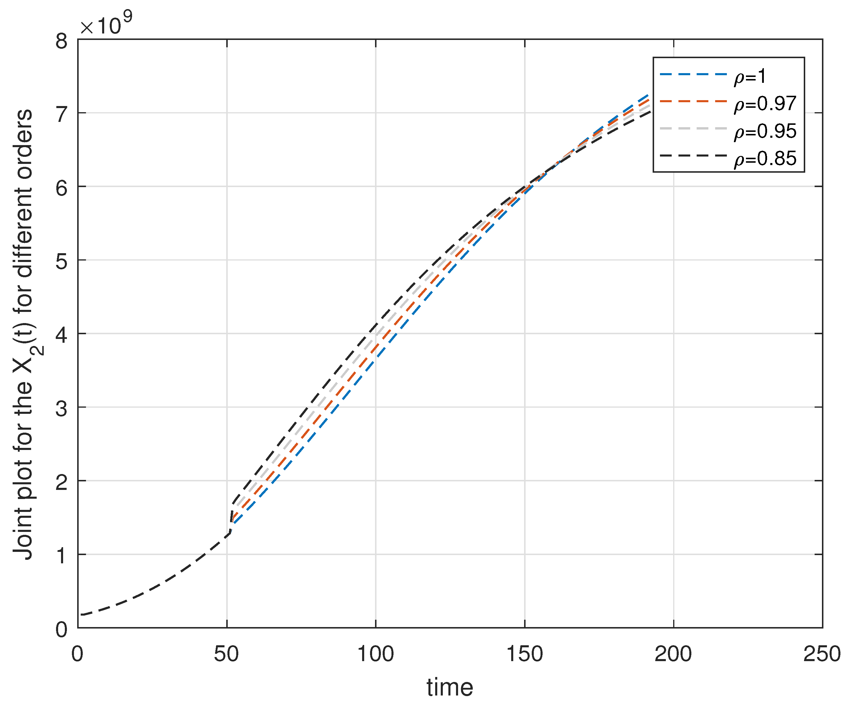
The simulations are carried out in the figures and explained here. Our proposed differential operator and integral operator are in the piecewise combination of the classical and the modified ABC operators. For this, we have considered the interval of study as for two hundred units; that is, $I=[0,200]$. This interval is divided into two subintervals. The first is $I_1=[0,50]$ and the second is $[50,200]$. Thus, $t_1=50$ while $t_2=200$. The first graph is for $X_1\left(t\right)$, in which we can see the simulations for the dynamics are representing the crossover behavior given in the Figure 1. This class shows a sudden fall in its population after 100 days. The fractional orders are considered in the second subinterval $[50,200]$. Crossover behavior is apparently observed in the simulations. In Figure 2 that follows, we have dynamics for the $X_2$, which is described in two intervals ${\mathcal{I}}_1$ and ${\mathcal{I}}_2$. In the ${\mathcal{I}}_1$, the dynamics are presented for the classical derivative of order 1, while in the second interval ${\mathcal{I}}_2$, the modified ABC fractional derivative is considered. A clear crossover behavior of the $X_2$ is observed at the time 50. The fractional orders are considered as $1,0.95,0.90,0.85$. There is initially an increase in leukemic cells. In Figure 3, the chemotherapeutic agents are presented, which are decreasing with respect to the time. In these three figures, we have considered the reproduction of normal cells and leukemic cells identical as ${\psi }_n={\psi }_l=0.04$ and per the references [15,16]. In the next three figures, we have presumed that ${\psi }_n={\psi }_l=0.08$, which affects the fall in the accumulation of normal cells, and there is a comparatively rapid increase in leukemic cells, which can be observed in the Figure 4 and Figure 5, respectively.

In Figure 1, we have given results for the $X_1$, which represents the class of normal cells.

7. Conclusions

In this article, a leukemia piecewise fractional-order model is constructed and presented for theoretical as well computational works. In theoretical works, the theory of fixed points is considered for the solution existence, and solution uniqueness and stability are obtained with the classical notions. The numerical work is based on our computational scheme carried out with the help of Lagrange’s polynomial. The model is studied for two different cases. In the first case, we have considered the values of ${\psi }_n={\psi }_l=0.04$, as per classical case. And the computational results are presented in three graphs as Figure 1, Figure 2 and Figure 3. Then, the values are modified to ${\psi }_n={\psi }_l=0.08$, and further new computations are presented in Figure 4, Figure 5 and Figure 6. With the increase in these values, we observe the loss in the normal cells with a further increase and the shift to leukemia growth, which even falls under the role of chemotherapy. Recent chemotherapeutic developments in leukemia have opened up promising new treatment options for patients. Due to their remarkable effectiveness, targeted treatments, immunotherapies, and combination regimens are gradually displacing conventional chemotherapy in some patient populations. Drug resistance and toxicity are two problems that still need to be addressed. To further improve the efficacy and safety of leukemia chemotherapy, future studies should concentrate on improving treatment regimens, discovering predictive biomarkers, and generating novel drugs. One can extend the work in the stochastic version with the help of [50].

References

- Doebelin, E. System Dynamics: Modeling, Analysis, Simulation, Design; CRC Press: Boca Raton, FL, USA, 1998. [Google Scholar]
- Castillo-Chavez, C.; Song, B. Dynamical models of tuberculosis and their applications. Math. Biosci. Eng. 2004, 1, 361–404. [Google Scholar] [CrossRef]
- Velten, K. Mathematical Modeling and Simulation: Introduction for Scientists and Engineers; John Wiley & Sons: Hoboken, NJ, USA, 2009. [Google Scholar]
- Formaggia, L.; Quarteroni, A.; Veneziani, A. Cardiovascular Mathematics: Modeling and Simulation of the Circulatory System; Springer Science & Business Media: Berlin/Heidelberg, Germany, 2010. [Google Scholar]
- Bunimovich-Mendrazitsky, S.; Kronik, N.; Vainstein, V. Optimization of Interferon–Alpha and Imatinib Combination Therapy for Chronic Myeloid Leukemia: A Modeling Approach. Adv. Theory Simul. 2019, 2, 1800081. [Google Scholar] [CrossRef]
- Khatun, M.S.; Biswas, M.H. Modeling the effect of adoptive T cell therapy for the treatment of leukemia. Comput. Math. Methods 2020, 2, e1069. [Google Scholar] [CrossRef] [Green Version]
- Piller, G. The history of leukemia: A personal perspective. Blood Cells 1993, 19, 521–529. [Google Scholar] [PubMed]
- Drexler, H.G.; Minowada, J. History and classification of human leukemia-lymphoma cell lines. Leuk. Lymphoma 1998, 31, 305–316. [Google Scholar] [CrossRef] [PubMed]
- Thomas, X. First contributors in the history of leukemia. World J. Hematol. 2013, 2, 62–70. [Google Scholar] [CrossRef]
- Mehranfar, S.; Zeinali, S.; Hosseini, R.; Mohammadian, M.; Akbarzadeh, A.; Feizi, A.H. History of leukemia: Diagnosis and treatment from beginning to now. Galen Med. J. 2017, 6, 12–22. [Google Scholar] [CrossRef]
- Afenya, E. Acute leukemia and chemotherapy: A modeling viewpoint. Math. Biosci. 1996, 138, 79–100. [Google Scholar] [CrossRef] [PubMed]
- Khatun, M.S.; Biswas, M.H. Mathematical analysis and optimal control applied to the treatment of leukemia. J. Appl. Math. Comput. 2020, 64, 331–353. [Google Scholar] [CrossRef]
- Nobile, M.S.; Vlachou, T.; Spolaor, S.; Bossi, D.; Cazzaniga, P.; Lanfrancone, L.; Mauri, G.; Pelicci, P.G.; Besozzi, D. Modeling cell proliferation in human acute myeloid leukemia xenografts. Bioinformatics 2019, 35, 3378–3386. [Google Scholar] [CrossRef] [Green Version]
- Li, Y.F.; Combes, F.P.; Hoch, M.; Lorenzo, S.; Sy, S.K.; Ho, Y.Y. Population pharmacokinetics of asciminib in tyrosine kinase inhibitor-treated patients with Philadelphia chromosome-positive chronic myeloid leukemia in chronic and acute phases. Clin. Pharmacokinet. 2022, 61, 1393–1403. [Google Scholar] [CrossRef] [PubMed]
- Islam, Y.; Ahmad, I.; Zubair, M.; Shahzad, K. Double integral sliding mode control of leukemia therapy. Biomed. Signal Process. Control 2020, 61, 102046. [Google Scholar] [CrossRef]
- Islam, Y.; Ahmad, I.; Zubair, M.; Islam, A. Adaptive terminal and supertwisting sliding mode controllers for acute Leukemia therapy. Biomed. Signal Process. Control 2022, 71, 103121. [Google Scholar] [CrossRef]
- Awadalla, M.; Subramanian, M.; Abuasbeh, K. Existence and Ulam–Hyers Stability Results for a System of Coupled Generalized Liouville–Caputo Fractional Langevin Equations with Multipoint Boundary Conditions. Symmetry 2023, 15, 198. [Google Scholar] [CrossRef]
- Alesemi, M.; Shahrani, J.S.; Iqbal, N.; Shah, R.; Nonlaopon, K. Analysis and Numerical Simulation of System of Fractional Partial Differential Equations with Non-Singular Kernel Operators. Symmetry 2023, 15, 233. [Google Scholar] [CrossRef]
- Baitiche, Z.; Benchohra, C.D.C.M.; Zhou, Y. A New Class of Coupled Systems of Nonlinear Hyperbolic Partial Fractional Differential Equations in Generalized Banach Spaces Involving the ψ–Caputo Fractional Derivative. Symmetry 2021, 13, 2412. [Google Scholar] [CrossRef]
- Srinivasa, K.; Baskonus, H.M.; Sanchez, Y.G. Numerical solutions of the mathematical models on the digestive system and COVID-19 pandemic by hermite wavelet technique. Symmetry 2021, 13, 2428. [Google Scholar] [CrossRef]
- Atangana, A.; Araz, S.I. New concept in calculus:Piecewise differential and integral operators. Chaos Solitons Fractals 2021, 145, 110638. [Google Scholar] [CrossRef]
- Ahmad, S.; Yassen, M.F.; Alam, M.M.; Alkhati, S.; Jarad, F.; Riaz, M.B. A numerical study of dengue internal transmission model with fractional piecewise derivative. Results Phys. 2022, 39, 105798. [Google Scholar] [CrossRef]
- Heydari, M.H.; Razzaghi, M.; Baleanu, D. A numerical method based on the piecewise Jacobi functions for distributed-order fractional Schrödinger equation. Commun. Nonlinear Sci. Numer. Simul. 2023, 116, 106873. [Google Scholar] [CrossRef]
- Kafle, R.C.; Kim, D.Y.; Holt, M.M. Gender-specific trends in cigarette smoking and lung cancer incidence: A two-stage age-stratified Bayesian joinpoint model. Cancer Epidemiol. 2023, 84, 102364. [Google Scholar] [CrossRef]
- Abdelmohsen, S.A.M.; Yassen, M.F.; Ahmad, S.; Abdelbacki, A.M.M.; Khan, J. Theoretical and numerical study of the rumours spreading model in the framework of piecewise derivative. Eur. Phys. J. Plus 2022, 137, 738. [Google Scholar] [CrossRef]
- Xu, C.; Liu, Z.; Pang, Y.; Akgul, A.; Baleanu, D. Dynamics of HIV-TB coinfection model using classical and Caputo piecewise operator: A dynamic approach with real data from South-East Asia, European and American regions. Chaos Solitons Fractals 2022, 165, 112879. [Google Scholar] [CrossRef]
- Hasan, A.; Akgul, A.; Farman, M.; Chaudhry, F.; Sultan, M.; De la Sen, M. Epidemiological Analysis of Symmetry in Transmission of the Ebola Virus with Power Law Kernel. Symmetry 2023, 15, 665. [Google Scholar] [CrossRef]
- Shah, A.; Khan, H.; De la Sen, M.; Alzabut, J.; Etemad, S.; Deressa, C.T.; Rezapour, S. On Non-Symmetric Fractal-Fractional Modeling for Ice Smoking: Mathematical Analysis of Solutions. Symmetry 2022, 15, 87. [Google Scholar] [CrossRef]
- Feng, Y.; Yu, J. Lie symmetry analysis of fractional ordinary differential equation with neutral delay. AIMS Math. 2021, 6, 3592–3605. [Google Scholar] [CrossRef]
- Liu, Y. On piecewise continuous solutions of higher order impulsive fractional differential equations and applications. Appl. Math. Comput. 2016, 287, 38–49. [Google Scholar] [CrossRef]
- Ansari, K.J.; Asma; Ilyas, F.; Shah, K.; Khan, A.; Abdeljawad, T. On new updated concept for delay differential equations with piecewise Caputo fractional-order derivative. Waves Random Complex Media 2023, 1–20. [Google Scholar] [CrossRef]
- Angstmann, C.N.; Henry, B.I.; Jacobs, B.A.; McGann, A.V. Discretization of fractional differential equations by a piecewise constant approximation. Math. Model. Nat. Phenom. 2017, 12, 23–36. [Google Scholar] [CrossRef] [Green Version]
- Al-Refai, M.; Baleanu, D. On an Extension of the Operator with Mittag-Leffler Kernel. Fractals 2022, 30, 1–7. [Google Scholar] [CrossRef]
- Al-Refai, M. Proper inverse operators of fractional derivatives with nonsingular kernels. Rend. Del Circ. Mat. Palermo Ser. 2022, 71, 525–535. [Google Scholar] [CrossRef]
- Khan, A.; Abdeljawad, T.; Gomez-Aguilar, J.F.; Khan, H. Dynamical study of fractional order mutualism parasitism food web module. Chaos Solitons Fractals 2020, 134, 109685. [Google Scholar] [CrossRef]
- Khan, H.; Alzabut, J.; Gulzar, H. Existence of solutions for hybrid modified ABC-fractional differential equations with p-Laplacian operator and an application to a waterborne disease model. Alex. Eng. J. 2023, 70, 665–672. [Google Scholar] [CrossRef]
- Boutiara, A.; Matar, M.M.; Alzabut, J.; Samei, M.E.; Khan, H. On ABC coupled Langevin fractional differential equations constrained by Perov’s fixed point in generalized Banach spaces. AIMS Math. 2023, 8, 12109–12132. [Google Scholar] [CrossRef]
- Khan, H.; Alzabut, J.; Baleanu, D.; Alobaidi, G.; Rehman, M.U. Existence of solutions and a numerical scheme for a generalized hybrid class of n-coupled modified ABC-fractional differential equations with an application. AIMS Math. 2023, 8, 6609–6625. [Google Scholar] [CrossRef]
- Khan, A.; Ain, Q.T.; Abdeljawad, T.; Nisar, K.S. Exact Controllability of Hilfer Fractional Differential System with Non-instantaneous Impluleses and State Dependent Delay. Qual. Theory Dyn. Syst. 2023, 22, 62. [Google Scholar] [CrossRef]
- Djaout, A.; Benbachir, M.; Lakrib, M.; Matar, M.M.; Khan, A.; Abdeljawad, T. Solvability and stability analysis of a coupled system involving generalized fractional derivatives. AIMS Math. 2023, 8, 7817–7839. [Google Scholar] [CrossRef]
- Thirthar, A.A.; Abboubakar, H.; Khan, A.; Abdeljawad, T. Mathematical modeling of the COVID-19 epidemic with fear impact. AIMS Math. 2023, 8, 6447–6465. [Google Scholar] [CrossRef]
- Houas, M.; Kaushik, K.; Kumar, A.; Khan, A.; Abdeljawad, T. Existence and stability results of pantograph equation with three sequential fractional derivatives. AIMS Math. 2023, 8, 5216–5232. [Google Scholar] [CrossRef]
- Khan, A.; Shah, K.; Abdeljawad, T.; Alqudah, M.A. Existence of results and computational analysis of a fractional order two strain epidemic model. Results Phys. 2022, 39, 105649. [Google Scholar] [CrossRef]
- Scholtes, S. Introduction to Piecewise Differentiable Equations; Springer Science & Business Media: Berlin/Heidelberg, Germany, 2012. [Google Scholar]
- Tanvi, A.; Aggarwal, R.; Raj, Y.A. A fractional order TB co-infection model in the presence of exogenous reinfection and recurrent TB. Nonlinear Dyn. 2021, 104, 4701–4725. [Google Scholar]
- Zeb, A.; Alzahrani, A. Non-standard finite difference scheme and analysis of smoking model with reversion class. Res. Phys. 2021, 21, 103785. [Google Scholar] [CrossRef]
- Srivastava, H.M.; Gusu, D.M.; Mohammed, P.O.; Wedajo, G.; Nonlaopon, K.; Hamed, Y.S. Solutions of general fractional-order differential equations by using the spectral Tau method. Fractal Fract. 2022, 6, 7. [Google Scholar] [CrossRef]
- Youssri, Y.H.; Abd-Elhameed, W.M.; Ahmed, H.M. New fractional derivative expression of the shifted third-kind Chebyshev polynomials: Application to a type of nonlinear fractional pantograph differential equations. J. Funct. Spaces 2022, 2022, 3966135. [Google Scholar] [CrossRef]
- Doha, E.; Abd-Elhameed, W.M.; Ahmed, H. The coefficients of differentiated expansions of double and triple Jacobi polynomials. Bull. Iran. Math. Soc. 2012, 38, 739–765. [Google Scholar]
- Ain, Q.T.; Nadeem, M.; Akgul, A.; De la Sen, M. Controllability of Impulsive Neutral Fractional Stochastic Systems. Symmetry 2022, 14, 2612. [Google Scholar] [CrossRef]
Figure 1.
Graphical representation of in piecewise model (1) with keeping .
Figure 2.
Figure 3.
Figure 4.
Figure 5.
Figure 6.
Disclaimer/Publisher’s Note: The statements, opinions and data contained in all publications are solely those of the individual author(s) and contributor(s) and not of MDPI and/or the editor(s). MDPI and/or the editor(s) disclaim responsibility for any injury to people or property resulting from any ideas, methods, instructions or products referred to in the content. |
© 2023 by the authors. Licensee MDPI, Basel, Switzerland. This article is an open access article distributed under the terms and conditions of the Creative Commons Attribution (CC BY) license (https://creativecommons.org/licenses/by/4.0/).
Share and Cite
MDPI and ACS Style
Khan, H.; Alzabut, J.; Alfwzan, W.F.; Gulzar, H. Nonlinear Dynamics of a Piecewise Modified ABC Fractional-Order Leukemia Model with Symmetric Numerical Simulations. Symmetry 2023, 15, 1338. https://doi.org/10.3390/sym15071338
AMA Style
Khan H, Alzabut J, Alfwzan WF, Gulzar H. Nonlinear Dynamics of a Piecewise Modified ABC Fractional-Order Leukemia Model with Symmetric Numerical Simulations. Symmetry. 2023; 15(7):1338. https://doi.org/10.3390/sym15071338
Chicago/Turabian StyleKhan, Hasib, Jehad Alzabut, Wafa F. Alfwzan, and Haseena Gulzar. 2023. "Nonlinear Dynamics of a Piecewise Modified ABC Fractional-Order Leukemia Model with Symmetric Numerical Simulations" Symmetry 15, no. 7: 1338. https://doi.org/10.3390/sym15071338
Note that from the first issue of 2016, this journal uses article numbers instead of page numbers. See further details here.