
Heat Transfer Models and Measurements of Brushless DC Motors for Small UASs


Department of Aerospace Engineering, Texas A&M University, College Station, TX 77840, USA
*
Author to whom correspondence should be addressed.
Aerospace 2024, 11(5), 401; https://doi.org/10.3390/aerospace11050401
Submission received: 19 February 2024
/
Revised: 13 May 2024
/
Accepted: 14 May 2024
/
Published: 16 May 2024
(This article belongs to the Special Issue Aircraft Design (SI-5/2023))
Abstract
:Heat transfer affects a motor’s sizing, its performance, and, ultimately, the overall vehicle’s range and endurance. However, the thermal literature does not have early-stage models for outrunner brushless DC (BLDC) motors found in small unmanned aerial systems (UASs). To address this gap, we have developed a non-dimensional heat transfer model (Nusselt correlation). Parametric experiments of four different-sized BLDC motors under load in Reynolds-matched wind tunnel tests generated data for model correlation. The motors’ aspect ratios (diameter/length) ranged from 0.9 to 1.5. The freestream Reynolds number of the axial flow over the motors ranged from 20,000 to 40,000. The rotational Reynolds number ranged from 10,000 to 20,000. The results showed that aspect ratio had the largest influence on heat transfer, followed by rotational and freestream Reynolds numbers. A steady-state model used the correlation to predict the motor’s ambient temperature differential within 10 K of experimental data. A case study applied the correlation to predict a hypothetical motor’s continuous torque in different environments. The correlation enables conceptual designers to capture thermally-driven trade-offs in early design stages and reduce costly revisions in later stages.

1. Introduction
Motor heat transfer affects a vehicle’s high-level metrics like gross weight, endurance, and range. A small, actively-cooled brushless DC (BLDC) motor can deliver as much torque and power as a large, passively-cooled BLDC motor. A small unmanned aerial system (UAS) with smaller motors could be lighter and fly farther and longer. However, vehicle conceptual designers do not have practical tools to model size, performance, and thermal trade-offs for an arbitrary motor in different environments. Therefore, engineers must rely on experimental tests, which are expensive and time-consuming.
We developed analytical heat transfer models to predict the thermal response of an arbitrary-sized outrunner BLDC motor in any environment. The model inputs are high-level parameters that users can populate from commercial datasheets or other first-order models, such as steady-state efficiency models. Therefore, the heat transfer models are practical at the early design stages and enable users to evaluate a range of designs quickly.
We regressed and validated the models from parametric experimental studies of different-sized motors in Reynolds-matched flows. We built a test stand to characterize the motors in varying flow conditions inside a wind tunnel. The motors varied in size and aspect ratio (), which is the ratio of the motor’s diameter (D) to its length (L), as defined in Equation (1). We adjusted wind tunnel freestream velocity () and motor rotational speed () in each test case to match freestream Reynolds number (, Equation (2)) and rotational Reynolds number (, Equation (3)), respectively, for the different motors. We used some data to regress non-dimensional heat transfer (Nusselt) correlations that we validated against the remaining (non-correlated) data.
The models and test data are limited to axially air-cooled BLDC motors in small UASs. The experimental results and numerical correlations apply to outrunner motors driving suitably sized propellers in Reynolds-matched axial and rotation flow. However, readers can extend the experimental methodology and analysis to study other motors and components, such as the motor controller or battery.
Thermal models are inherently sensitive to the geometry and flow configuration because heat transfer is an extrinsic process. Previous research, such as Ref. [1], correlated heat transfer between the elements inside BLDC motors of varying geometry. However, conceptual designers need models to predict heat transfer to the external environment. Conversely, Ref. [2] studied the external heat transfer between two motors of constant aspect ratio. However, this correlation cannot account for different motor geometries. We studied the external heat transfer in multiple motors with varying aspect ratios in a flow configuration that closely matches a motor’s configuration on a small UAS. Our results are more practical to vehicle conceptual designers who seek to evaluate the external heat transfer of a range of motor concepts in early design.
Researchers will appreciate the experimental methodology and parametric results. They can improve the framework to validate our results further and test other devices. They can also develop other models from our experimental results. The results may even prove valuable to electric machine and heat transfer researchers exploring novel designs for electric aviation [3].
Practitioners will appreciate the experimental results and analytical models. They can use the models to evaluate an existing or conceptual motor’s performance in different environments. Application engineers can use the experimental data as a reference for existing motors and aircraft designs. Even motor designers could use the analytical models and experimental data to analyze new outrunner BLDC motor designs.
1.1. Motivation
A BLDC motor converts electrical power in its stator to mechanical power out of its rotor via magnetic interactions. Current enters select stator windings and generates a magnetic field around the stator. The rotor’s permanent magnets (Figure 1) seek to align with the stator field, and the resulting magnetic forces apply a net torque on the shaft that spins the rotor. Other motor types, such as induction or axial-flux motors, rely on different approaches to generate the stator–rotor magnetic interactions. References [4,5,6] discuss these differences in more detail.
The motor design literature shows that a motor’s size, output performance, and thermal response are all coupled. In Equation (4), the output torque (M) is a function of the input electromagnetic loading () and the motor volume (U) [7]. Input loading is a function of the input current (I) [8] and is implicitly limited by heat transfer (cooling). Loading generates internal losses, such as Joule losses (), that can increase motor temperature beyond critical limits without adequate cooling. These limits include the demagnetization temperature (Curie temperature) of the rotor’s permanent magnets [9]. Assuming that mass is proportional to volume (), a small (light) motor with high loading could deliver as much torque as a large (heavy) motor with low loading () if the lighter motor receives sufficient cooling. A vehicle with lighter motors could extract more endurance and range from its battery. Reference [10] discusses BLDC motor losses in more detail and develops a flight-validated model to predict them.
Unfortunately, conceptual designers lack viable tools or data to evaluate motor thermal effects. Some existing approaches are too cumbersome for early design stages. Other approaches focus on inappropriate heat transfer regions or are limited to a single point design. Moreover, designers cannot rely on motor datasheets for consistent comparisons.
Traditional motor thermal modeling tools, such as MotorCAD, are too detailed for conceptual designers. These tools rely on high-fidelity thermal circuits to predict the local temperature transients in a BLDC motor under specified loads in a given environment [11]. These tools can predict if and where a motor will overheat at the specified loading and available cooling. However, the tools require input parameters—such as magnetic hysteresis curves or the number of winding turns per tooth—that are beyond the scope of a conceptual designer. Moreover, these computationally intensive tools may be too slow to conduct parametric sweeps for trade studies of many designs. Therefore, these tools are more appropriate for thermal engineers or motor designers analyzing a single motor concept at the detailed design stage.
The datasheets of commercial motors do not help compare the thermal trade-offs of existing motors. Small UAS motors are typically sourced from hobbyist manufacturers, and these fabricators do not specify the torque limits of their motors [12]. Some manufacturers may specify current ratings, but these figures are referenced with respect to different—and, sometimes, unspecified—limit criteria. One manufacturer lists a “max continuous” current limit for 3 min [12], while another lists a “peak” current limit with no time period [13]. Neither vendor specifies the freestream temperature or airspeed. An engineer cannot accurately compare the motors’ specifications.
The lack of appropriate thermal tools and data manifests in small UAS design tools that ignore a motor’s thermal response. Equation (4) shows that specific torque is effectively a variable function of cooling (electric loading). However, approaches in the small UAS design literature size motors using a constant-specific torque [14,15] or even a constant-specific power [16,17]. Moreover, these constant-specific performance metrics are derived from the aforementioned unreliable datasheets. Thus, the regressions have two sources of thermal uncertainty: statistical data collected at mismatched thermal settings and regressions that ignore cooling.
Steady-state thermal analysis could address the capability gap. The first-order expression in Equation (5) defines the convective cooling mode that dominates BLDC motor heat transfer. Convective heat transfer () is a function of the convective heat transfer coefficient (h), heat transfer surface area (A), and the temperature differential (, Equation (6)) between the motor () and the freestream flow ().
If we could dynamically predict h, we could evaluate whether a notional motor overheats under load in a specific environment. At steady-state, a motor dissipates all its internal losses to its surroundings (). We could solve Equation (5) for the motor’s steady-state temperature () given its geometry, losses, and freestream temperature. Unfortunately, predicting the heat transfer coefficient is difficult because h is an extrinsic property that depends on a body’s geometry and the external flow conditions [18].
1.2. Literature Review
The thermal literature outlines a fast analytical approach to heat transfer coefficient from salient non-dimensional thermal correlations. This approach is well-suited for conceptual designers because it can derive h from high-level parameters that a designer can obtain in early design stages, such as motor diameter and freestream velocity. In contrast, cumbersome computational thermal models like MotorCAD need motor design details beyond the scope of a vehicle designer at the conceptual design stage, such as a motor’s inner geometry and constituent material properties [19].
The literature analytical approach to estimating the heat transfer coefficient revolves around the non-dimensional Nusselt number (). Nusselt number is a non-dimensional measure of convection that scales to different flows and fluids [20]. Equation (7) defines the Nusselt number as a function of convective heat transfer coefficient (h), a characteristic length over a hot body (), and the ambient fluid’s thermal conductivity (). A Nusselt number greater than 1 ( > ) indicates that the fluid absorbs more heat via convection rather than conduction. Thus, a “good” convective system should have >> 1.
Researchers have correlated the Nusselt number to the non-dimensional Reynolds and Prandtl numbers for various canonical flows, as expressed in Equation (8) [18]. The Reynolds number () accounts for the viscous properties of different speeds and lengths, while the Prandtl number () accounts for the thermal properties of various fluids. Sometimes, is only correlated as a function of since for most gases [18].
For example, Equation (9) predicts the Nusselt number as a function of the freestream Reynolds number for a flat plate in freestream flow [21,22]. However, this Nusselt correlation is missing the rotation flow generated by a spinning motor. Conversely, Equation (10) defines the Nusselt number for a rotating cylinder as a function of the rotational Reynolds number [22,23]. This flow is missing the axial flow experienced by a small UAS motor.
Nusselt correlations can encompass hybrid flows that include axial and rotation components. Studies examined axial flow impinging onto a rotating flat disk [24,25], which is similar to the axial and rotation flow experienced by motors. The resulting correlation (Equation (11)) included an axial (freestream) Reynolds number and a rotational Reynolds number. Their correlation is inappropriate for small UAS motors since a motor is not a flat disk. Nonetheless, this study informed our experimental methodology to examine axial and rotation flow over a motor.
Historic correlations for industrial motors are inappropriate because small UAS motors fundamentally differ in design and operation. Traditional induction motors with an inner-rotor (inrunner) rely on stator fins to passively convect heat to surrounding air. Brushless motors with an outer rotor (outrunner) rely on the passing airflow to actively convect heat away from the rotor and stator. Otherwise, the literature contains empirical correlations developed over decades for traditional motors [26].
Some of the more recent literature that is focused on modern brushless motors ignores the forced axial airflow. A review paper on state-of-the-art electric motor modeling suggests Nusselt correlations that only examine the rotation flow around a motor [27]. Again, this type of correlation is inaccurate for most small UAS motors because such motors experience freestream (axial) and rotational flow. Rotational-only correlations [28] may suffice for electric motors in less-popular small electric helicopters wherein the motor is nestled inside the vehicle and does not receive external airflow.
The other recent literature examines heat transfer between a motor’s internal elements rather than between the motor and its surroundings. For example, extensive analytical [29], computational [1,30], and experimental [31,32] studies examine heat transfer in the air gap between a brushless motor’s stator and rotor wherein motors generate torque. These studies explore different motor aspect ratios and consider axial and rotation air flows. However, their correlations are helpful for motor designers who are interested in maximizing localized heat transfer within different parts of the motor, such as the air gap.
The correlations from these studies are unsuitable for aircraft designers who seek to estimate heat transfer concerning surroundings. The flow inside a motor fundamentally differs from the fluid flow surrounding a motor. Cooling between a motor’s stationary stator and its rotating rotor is similar to the Taylor–Couette flow in two concentric cylinders, whereas cooling between a motor and its surroundings is a single cylinder in external flow. Nonetheless, the parametric exploration of different motor aspect ratios and Reynolds numbers informed the experimental methodology in this study.
The literature on a brushless motor’s external heat transfer is not as extensive as the literature on internal heat transfer. Reference [2] only studies external airflow for a single aspect ratio. There is no indication of how data would change for different aspect ratio motors. The same shortcoming applies to References [33,34], which are computational and experimental studies of a single motor design. A conceptual designer cannot extend their findings to an arbitrarily shaped motor.
The thermal literature would benefit from a parametric study of different-shaped motors operating in a mixed axial and rotation flow range. Such flows better reflect the external conditions in which a small UAS motor dissipates losses to its surroundings. Therefore, the resulting Nusselt correlations would be more practical for aircraft designers. The external heat transfer correlation would also help parameterize thermal modeling tools, such as MotorCAD. These late-stage tools can predict the temperature dynamics of different locations on a motor. However, a user must still supply the expected heat transfer coefficient (h) for different regions because the tools do not predict h [11]. Rather, the tools’ governing equations use h to solve for temperature. Literature models developed in Refs. [1,29,30] could populate h for the internal heat transfer surfaces, and an external heat transfer correlation could populate h for external heat transfer surfaces.
2. Methodology
The test stand in Figure 2 generated experimental data per the approach visualized in Figure 3. Section 2.1, Section 2.2 and Section 2.3 discuss the stand, the tested motors, and the stand’s instrumentation, respectively, in more detail. For each test motor (Section 2.2), a Latin hypercube sampler selected 10 points from the 2D Reynolds domain (Section 2.4). The motor operated under load in the wind tunnel at the corresponding freestream velocity and rotational speed until it reached thermal steady-state (Section 2.7), which populated steady-state data for numerical correlation (Section 2.8).
2.1. Wind Tunnel Stand
The wind tunnel test stand shown in Figure 2 characterized outrunner motors driving a propeller in axial flow. The wind tunnel could generate freestream flows ranging from 4 to 20 m/s (8 to 39 kn). The test section was 0.91 m tall and 1.23 m wide (3 ft × 4 ft). A built-in environmental control system maintained freestream temperature () at 23.5 °C. A key feature, which is not visible in this figure, is the three-phase power analyzer that measured electrical power entering the motor. This device was located below the wind tunnel test section to avoid disturbing the flow.
Fixed-pitch propellers applied the necessary load to the test motors. The motor–propeller pairing followed recommendations from the motor manufacturer regarding propeller diameter and the number of blades. The propeller’s applied torque changed as the wind tunnel velocity changed for a constant propeller speed. This load-flow coupling had broader implications on the heat transfer study, which Section 2.6 discusses. The axial flow configuration is typical of the widest variety of electric aircraft, including fixed-wing airplanes and rotorcraft in axial climb.
2.2. Tested Motors
Table 1 lists the four test motors. Motors 1 and 2 have different diameters (D) but roughly similar lengths (L). Conversely, motors 3 and 4 have identical diameters but various lengths. All motors have the same general shape and features as those pictured in Figure 4. Each motor’s rotor has slots on the front that impel some air into the motor and over the stator windings. References [1,29,31] study this internal heat transfer. The reference citations for each motor link to its full datasheet. A motor controller with a programmable governor regulated rotational speed for all motors [35].
2.3. Instrumentation
The instrumentation system abstracted in Figure 5 measured salient time-varying electrical, mechanical, and thermal parameters. A National Instruments data-acquisition board (DAQ) and LabVIEW 2019 software (Austin, TX, USA) sampled and recorded the readings at 1 Hz. Tests lasted on the order of minutes, depending on the applied load and freestream velocity. A Figshare repository contains the transient test data (see link in Data availability).
A torque sensor and a tachometer measure the motor’s output torque () and rotational speed (), respectively. The product of these readings yielded the motor’s output mechanical power (, Equation (12)). A three-phase power analyzer measured the motor’s input electrical power (). The difference between the motor’s input and output power yielded the motor’s losses (, Equation (13)).
K-type thermocouples measure the motor temperature () and the freestream air temperature (). The thermocouple, which measures motor temperature, is bonded inside the motor with thermal cement, as shown in Figure 6. The difference between these temperature measurements yields the motor’s instantaneous temperature differential with respect to freestream temperature (, Equation (6)).
2.4. Control Variables
Three non-dimensional numbers served as control variables in this study:
The lower and upper bounds of our study’s Reynolds domain stemmed from wind tunnel and motor controller limits. The wind tunnel could not run slowly enough to generate < 20,000 for the largest motor or run fast enough to generate > 40,000 for the smallest motor. The motor controller did not have sufficient control authority to produce < 10,000 for the largest motor or > 20,000 for the smallest motors.
Latin hypercube sampling (LHS) maximized coverage within the two-dimensional Reynolds domain for a finite number of tests. For each motor, an LHS sampler selected ten combinations of freestream and rotational Reynolds numbers such that no two cases occupied the same freestream and rotational Reynolds numbers. This helped distinguish the influences of freestream and rotational Reynolds numbers on the Nusselt number. We then converted the non-dimensional Reynolds numbers into dimensional freestream velocity and rotational speed values for the wind tunnel and motor, respectively.
2.5. Assumptions
We assumed the following in this study:
- Convection was the motor’s sole mode of heat transfer. To enforce this assumption, we installed a layer of thermally non-conductive plastic (Delrin) between the aluminum motor housing and the aluminum test stand. Delrin’s thermal conductivity is 1000× smaller than aluminum’s (0.210 vs. 237 W/(m·K), respectively [40]). We ignored radiation;
- Convection only occurred along the motor’s lateral surface area. The propeller and propeller adapter impede airflow onto the front of the motor. Forced convection due to the freestream velocity and rotational speed dissipated losses along the lateral surface area as depicted in Figure 7;
- The fluid characteristic length was the motor’s diameter (). The heat transfer literature suggests setting the characteristic length as the volume-to-surface area ratio. The motor is approximately a cylinder, and its volume/surface area ratio is proportional to diameter: . Additionally, the electrical literature shows that a motor’s diameter drives torque more than its length (Equation (4)).
Figure 7.
Forced convection from the freestream () and rotational () flows was the sole mode of heat transfer, and the motor dissipated all losses () through its lateral surface area ().
Figure 7.
Forced convection from the freestream () and rotational () flows was the sole mode of heat transfer, and the motor dissipated all losses () through its lateral surface area ().

2.6. Limiting Trade-Off
We sacrificed matching heat flux to match the Reynolds number across all motors and test cases. Some studies in the thermal literature also match the heat transfer per unit area, or heat flux (, Equation (14)), across different test cases. However, we could not achieve this additional constraint because flux-matching with fixed-pitch propellers is not trivial. Controlling heat flux requires direct control over motor losses. Motor losses are driven primarily by torque [10], and a fixed-pitch propeller’s torque is coupled to the propeller’s rotational speed and the freestream airflow velocity. However, the rotational speed and flow velocity also affect the motor’s Reynolds numbers. Therefore, we could have matched the Reynolds number or heat flux, but not both.
The flux trade-off did not diminish our study’s utility. Any motor driving a propeller will experience these same dynamics as our tests, so the resulting data still applies. Moreover, the data will serve as a reference point for other research that will achieve flux matching. In Section 5.3, we discuss how a variable-pitch propeller actuated by a control system with feedback on motor losses could match flux and Reynolds numbers.
2.7. Steady-State Analysis
We extracted salient thermal parameters when the motor achieved a thermal steady state in each test. Recall that a test case was defined by the combination of axial speed () and rotational speed () derived from the Latin hypercube sampling described in the control variables subsection. We defined steady state as when the measured motor temperature changes less than 1 K/min during a test (Equation (15)). For each test case, we collected time-varying data on the motor’s losses () and freestream temperature differential (). When the motor temperature reached steady state, we calculated the steady-state losses, heat transfer coefficient (Equation (16)), and Nusselt number (Equation (17)). The instrumentation subsection details how we measured motor temperature and losses.
2.8. Numerical Correlation
We used linearized power-law regression to develop the Nusselt number correlations. Nusselt number is a nonlinear function of aspect ratio, freestream, and rotational Reynolds number, as expressed in Equation (18). Taking the natural log of both sides yields the multivariate linear expression in Equation (19). Equation (20) abstracts (19) for visual clarity. We then populated a system of equations (Equation (21)) with data from each motor (i) and each of its test cases (j). Finally, we solved for the unknown exponents (, , and ) and coefficient ().
2.9. Uncertainty Propagation
Equation (22) estimated the uncertainty of our Nusselt measurements. The uncertainties Python package [41] numerically calculated the solution to Equation (22) from the sensor uncertainties listed in Table 2. Equation (22) is derived from Equation (23), which defines Nusselt number as a function of the downstream sensor readings: torque (M), rotational speed (), electrical motor power (), and the freestream temperature differential (). Equation (23) is itself a derivation of Equation (7) with substitions from Equations (5), (12) and (13).
3. Results
First, we present experimental results for all cases. Then, a filter removes cases with high uncertainty for the measured Nusselt number. We develop a Nusselt correlation using some of the low-uncertainty instances, and we validate the correlation’s accuracy against the remaining (uncorrelated) experimental data. The comparisons also include predictions from salient literature models for reference.
Figure 8 plots all of the experimental test cases as a function of the three control variables: freestream Reynolds number (), rotational Reynolds number (), and the motor’s aspect ratio (). The x-axis is the freestream Reynolds number, the y-axis is the rotational Reynolds number, and the color bar is the aspect ratio. Almost all test cases fell within the target bounds (dashed box) of Figure 8 as desired. The Latin hypercube sampling successfully distributed test points for each aspect ratio motor across the Reynolds domain.
3.1. Reducing Uncertainty
Figure 9 plots the relative uncertainty of the measured Nusselt number for all the cases. The x-axis is , and the y-axis is . The color bar is the relative uncertainty of the measured Nusselt number (). A darker data point indicates larger uncertainty for the measured Nusselt number.
Figure 9 shows that the high freestream, low rotational Reynolds number cases had high Nusselt number uncertainty. This region corresponds to high freestream velocity and low rotational speed. Spinning a propeller in such conditions requires little torque and generates small losses. Therefore, the motor experienced only a slight increase in temperature that increased the Nusselt measurement’s uncertainty (Equation (22)).
Figure 10 overlays a temperature filter to the data presented in Figure 9 to remove 18 uncertain cases. The filter removed cases where < 10 K and > 80 °C. The steady-state criterion was < 1 K/min. Therefore, the filter only kept cases where the steady-state temperature differential was >10× the criterion’s resolution. The non-conductive delrin layer between the motor and stand had a maximum service temperature of 80 °C. Therefore, the filter excluded cases where the motor’s temperature exceeded this critical temperature at which conductive heat transfer may have begun.
3.2. Nusselt Correlation
Figure 11 plots measurements for the remaining cases with low relative Nusselt uncertainty. The x-axis is , the y-axis is , and the color bar is the measured Nusselt number (). The filter has reduced the range of rotational Reynolds numbers by almost 40%. The lowest case is practically 14,000 rather than the intended lower bound of 10,000. Nonetheless, most cases (22/40) remain, and seems to increase more clearly with rather than . However, the plot does not show the influence of aspect ratio.
Equation (24) is the non-linear power regression of the non-dimensional Nusselt number (), using 15 out of 22 randomly selected cases plotted in Figure 11. The regression has a residual standard error (RSE) of 41. The aspect ratio has the most decisive influence, followed by the rotational Reynolds number and then the freestream Reynolds number. The more substantial influence of compared to agrees with the visual trend in Figure 11, wherein tended to increase with .
3.3. Validation
We validate the correlation in Equation (24) against experimental data from various motors that were not used to develop the correlation. We also include predictions from the following four literature correlations for comparison. The following figures omit error bars for the literature models because their deviations are so large.
Equation (11) is the model Pelle developed for axial flow impinging on a rotating disk [24]. The regime of Pelle’s study (20,000 to 516,000) started where our regime ended (10,000 to 20,000). Nevertheless, this model is still insightful for comparisons since it considers the Nusselt number as a function of freestream and rotational flows. Notably, Pelle’s model shows a more substantial influence of freestream Reynolds number than rotational Reynolds number since the term has a more prominent exponent. This is the opposite of our correlation, wherein the term has a more prominent exponent.
Equation (10) models flow around a rotating cylinder developed by Etemad [23]. The regime of this study (700 to 10,000) ended where our regime started (10,000 to 20,000). Moreover, this study does not include any freestream flow. Nevertheless, this model is still insightful because it studies a rotating 3D cylinder that is similar to a brushless DC motor. The exponent of Etemad’s model (0.70) is only 6% higher than the exponent of the rotational Reynolds number in the proposed model (0.66 in Equation (24)), which increases confidence in the rotational aspect of our study.
Equation (9) is a canonical model developed by Pohlhausen for heat transfer over a flat plate in freestream flow [18]. The freestream and rotational flow around a 3D motor differ from the freestream flow over a flat plate. Nonetheless, we included this correlation because application engineers will often turn to this model as a point. The flat plate and Pelle correlations have identical exponents on the freestream term (0.50). The proposed correlation (Equation (24)) has a roughly 20% smaller exponent (0.39) on the freestream term, which might stem from the removal of uncertain data points at high .
Figure 12 plots Nusselt number (y-axis) versus rotational Reynolds number (x-axis) for experimental data and various models. The experimental data points were not used to develop the proposed correlation. The error bars for the experimental data are the estimated measurement uncertainty for the Nusselt number. The error bars on the proposed model data points represent the residual standard error (RSE).
Figure 12 shows that the proposed model predicts the Nusselt number more accurately and precisely than the literature models. For example, the experimental Nusselt number exhibits a local maximum for between 14,000 and 18,000. The proposed model captures this trend, whereas the other models do not. The Pelle model predicts a local minimum in this range, and the Etemad predictions barely change. We suspect the proposed model performs better than Pelle’s model because the former model also accounts for aspect ratio, which also changes for each data point. The proposed model probably performs better than Etemad’s model because the former model accounts for the changing aspect ratio and freestream Reynolds numbers.
Figure 13 plots Nusselt number (y-axis) versus freestream Reynolds number (x-axis). Again, the experimental data were not used to develop the proposed correlation. The experiment and model error bars represent measurement uncertainty and model residual standard error, respectively.
Figure 13 again shows that the proposed model predicts the Nusselt number more accurately and precisely than the literature models. The experimental Nusselt number experiences a local minimum for between 25,000 and 35,000, which the proposed model captures and the other models do not. The Pelle model suggests that the Nusselt number experiences a steady increase (no minimum), and the flat-plate predictions barely change. We hypothesize that the proposed model performs better because it accounts for the unseen variations in 3D geometry (), which Pelle’s model for a flat disk and the canonical model for a flat plate inherently cannot capture.
Figure 14 plots the heat transfer coefficient (y-axis) versus rotational speed (x-axis) for experimental and model data. The model predictions are obtained by solving for h in Equation (7) using the previously-predicted values. The experiment and model error bars represent measurement uncertainty and model residual standard error, respectively.
Figure 14 shows that dimensional predictions derived from the proposed model can accurately and precisely predict experimental trends. The experimental data experience a minimum of around 5800 min−1, which the proposed model reflects. Pelle’s model also exhibits this minimum; however, Pelle’s generally under-predicts the magnitude of h. Etemad’s model significantly under-predicts h and its variations.
Figure 15 plots heat transfer coefficient (y-axis) versus freestream velocity (x-axis) for experimental and model data. Again, model predictions are obtained via Equation (7). The experiment and model error bars represent measurement uncertainty and model residual standard error, respectively. The h vs. data in this figure reflect the same trend as the vs. data in Figure 13 because their axes are linearly proportional. Thus, Figure 15 suggests the same conclusions as Figure 13: the proposed model performs better because it accounts for freestream, rotational, and geometric influences on heat transfer.
Figure 16 plots temperature (y-axis) versus total motor losses (x-axis) for experimental and model data. The losses () are measured on the stand under different mechanical loading cases. The temperature predictions come from solving for in Equations (5) and (6) using the measured and the previously predicted h. The flat-plate and Etemad models significantly over-predict temperature by an order of magnitude because they under-predict heat transfer coefficient and Nusselt predictions further upstream. Nonetheless, the results suggest that the Etemad model, which is a function of , is relatively more accurate than the flat-plate model, which is a function of . This makes sense because our correlation revealed that motor Nusselt number is a more vital function of than .
Figure 17 zooms in on the more insightful <80 °C region in Figure 16. The axes and error bars are unchanged. Again, the proposed model performs better because its upstream h and predictions are more accurate. The residual standard error of the proposed model’s downstream temperature predictions is only 4 K. The proposed model achieves such accuracy despite two rounds of error propagation, which validates the proposed Nusselt correlation that is further upstream.
4. Case Study
What is the rated torque of a motor?
How does the rated torque change as the operating environment changes?
Designers cannot easily answer such questions because small UAS motors do not come with reliable torque and power ratings. These parts are typically sourced from hobbyist manufacturers, who provide inconsistent current ratings at best. For example, KDE Direct lists “maximum continuous current” ratings with a 3 min limit [12] while Scorpion lists “peak current” ratings with an unknown time limit [13]. Neither manufacturer specifies the operating speed, limit temperature, or ambient conditions associated with the current ratings; therefore, engineers cannot accurately compare performance metrics.
The block diagram in Figure 18 outlines the analytical methodology of this case study. The approach relies on the proposed thermal and efficiency models presented in Ref. [10]. The efficiency model predicts the steady-state losses of the motor under given loads. The computed losses will be the input to the thermal models, which predict the resulting steady-state temperature. Continuous torque is the region wherein the motor temperature does not exceed some critical limit, such as the Curie demagnetization temperature for rare-earth permanent magnets (120 °C [9]).
We analyzed a notional motor in the following environments:
- Cold environment with 10 m/s airflow at 20 °C;
- Hot environment with 5 m/s airflow at 40 °C.
The salient motor specifications are tabulated in Table 3. We assumed a limit temperature of 100 °C. The permanent magnets inside high-torque outrunner motors begin to demagnetize around 120 °C [42], and we applied a 20 °C buffer as a safety margin.
First, we predicted the motor’s losses and efficiency using the model in Equations (25) and (26), respectively. The model predicts losses () for a desired torque (M) and rotational speed () given the motor’s , , , and . The modeled losses include joule losses () associated with torque and iron losses () associated with rotational speed. The losses include approximate higher-order iron losses with a penalty proportional to 10% of the output power (). The joule and iron loss terms have an inverse amplification factor that is a function of the throttle setting (or duty ratio, d). This factor increases joule and iron losses at low throttle settings to approximate the harmonic distortions associated with regulating voltage to meet a desired rotational speed. The current is a function of the torque, torque constant, and no-load current: . The throttle setting (d) is a function of the motor’s torque constant, the desired speed, and the available voltage: . Our previous paper develops and validates the efficiency model against powertrain data from a flying quadcopter [10].
Figure 19 plots the efficiency model’s predictions over a prescribed rotational speed and torque window. The rotational speed range is 0–4000 min−1, and the torque range is 0–1000 N·mm. The dashed lines are lines of constant efficiency and show that efficiency tends to increase with higher rotational speeds. This is because joule losses (proportional to ) are the dominant source of losses for motors, and high-speed operation minimizes joule losses. Reference [10] discusses each source of motor losses in more detail.
Next, we predicted the steady-state temperature for the different environments using the expected losses (efficiency) and given specifications. We calculated the Nusselt number, heat transfer coefficient, and steady-state temperature.
Figure 20 plots the temperature predictions for the cold and hot environments. These plots’ x- and y-axes are rotational speed and torque, respectively. The dashed lines are lines of constant temperature. In both figures, the lowest-temperature region again corresponds to the low-torque, high-speed region. This region is not only the most efficient region due to low losses; it is also the best-cooled region thanks to higher rotational speed and, thereby, higher and h. The hot environment (Figure 20b) naturally reaches higher temperatures at the same operation conditions.
Figure 20 shows how the motor loses 25% of its rated torque going from the cold to the hot environment. In the cold case (Figure 20a), the motor can deliver up to 800 N·mm of torque at 3000 min−1 without exceeding the limit temperature. In the hot case (Figure 20b), the motor can only deliver 600 N·mm at the same rotational speed.
These results are more informative than the salient literature like motor datasheets. At best, commercial datasheets give inconsistent static ratings for “max” or “max continuous” current at vague or unspecified thermal reference frames. Conversely, our combined thermal and efficiency models dynamically predict the motor’s steady-state temperature under a range of torque and rotational speeds for a clearly defined ambient environment. With our model, a user can more confidently evaluate whether a motor is suitable for the desired application/environment.
Practitioners can extend our approach to rate and compare two motors from different manufacturers effectively. In this case study, we evaluated a single motor at two different thermal reference frames. Users can also virtually compare two motors at a single thermal reference frame using the same models. Users can model the devices under the same load, ambient temperature, and freestream airflow. Then, users can select whichever device has a lower steady-state temperature at the desired operating torque and rotational speed.
At a broader level, applications engineers can couple our proposed motor efficiency–thermal model with a vehicle model to dynamically predict vehicle performance changes induced by the environment. For example, a vehicle model could extend the changes in rated torque (and, thereby, rated power) from Figure 20 to predict changes in an electric vehicle’s payload capacity between cold and hot environments.
5. Discussion
First, we abstract actionable takeaways from the results and case studies. Next, we highlight novelties from the entire work, including the methodology. Finally, we discuss future steps to build on this work.
5.1. Key Takeaways
- Each motor’s thermal response is unique. Cooling is sensitive to flow conditions, motor rotational speed, and geometry. For example, Figure 11 shows two cases, both at roughly 25,000, 18,000. One case has a 300 while the other has 700, which is almost a twofold increase. These two points with nearly identical flow conditions vary in aspect ratio, as seen in Figure 8. Therefore, the dimensional heat transfer coefficient of the two motors of different sizes in similar flows will differ;
- Engineers should use Nusselt correlations carefully. Correlations are highly empirical, and a correlation developed for a body in one flow may not be appropriate for the same body in a different flow. Outrunner motors are rotating cylinders, yet Etemad’s correlation for such shapes (Equation (10)) significantly overestimates motor temperature in Figure 16. Engineers should strive to find a correlation that is based on a configuration that closely matches the configuration under consideration;
- Nameplate ratings are variable, not constant. “Continuous-”, “rated-”, and “limit-” torque ratings are not static parameters. A motor’s output torque is limited by its temperature, and the case study showed that the motor temperature varies with torque and rotational speed. Engineers can estimate the rated torque outside the manufacturer’s test points using our thermal and efficiency models;
- Electric motors suffer in hot environments just like combustion engines. In the case study, the motor reached its limit temperature at a lower torque in the hot environment than in the cold environment. The rotational speed was constant in both cases; therefore, the motor lost power in the hot case. This is analogous to how combustion engines develop less power in hot air. Designers can predict these changes using our models;
- Gearing can increase efficiency, improve cooling, and reduce weight. The case study showed how low torque and high speed increase efficiency and cooling. Torque is also the motor’s principle size driver [8], so trading torque for speed at a constant power also reduces size. Our thermal models can help engineers predict these improvements at the conceptual design stage.
5.2. Novel Contributions
We made the following contributions to the state-of-the-art:
- Novel methodology to characterize electric motor heat transfer in different freestream and rotational flow conditions. The approach allowed us to study motors of various sizes and match the freestream Reynolds and rotational Reynolds numbers. Our approach could not match heat flux across cases like traditional heat transfer studies. Nonetheless, the tested conditions reflect realistic loads and flow regimes and improve the literature. Reference [2] used a spinning cylinder containing a heating coil to simulate a motor. The study approximated motor losses from the current delivered to the coils. Our approach uses actual motors under load and directly measures the motor’s operating losses. Practitioners can use our methodology to test powertrains before flight tests and characterize the powertrain’s temperature response. Researchers can use the method to replicate and validate our results or develop new correlations;
- Novel experimental data on outrunner brushless DC motors’ heat transfer. We characterized the steady-state heat transfer of four different motors with unique aspect ratios under Reynolds-matched flows ( ranging from 20,000 to 40,000, ranging from 10,000 to 20,000). Our data improve on the literature, which only contains studies on single motors. For example, reference [43] conducted detailed experimental Particle Image Velocimetry (PIV) and computational fluid studies on the thermal and flow processes of a single fixed-size brushless DC motor. However, these results are of little use for conceptual designers who seek heat transfer data for a broad range of devices, which could vary in size and aspect ratio. Our experimental data sacrifice some fidelity for robustness to fill this gap in the literature. Practitioners can interpolate within our data and extrapolate our data’s trends to estimate the heat transfer of their motors without having to conduct any experiments. Researchers can use our data to validate other heat transfer models or evaluate the utility of other literature correlations;
- Novel Nusselt number correlations for the external heat transfer of brushless DC motors in rotational and axial (freestream) flow. Nusselt correlations are highly empirical, and literature correlations examine the internal heat transfer of brushless DC motors. For example, Ref. [30] derives a Nusselt correlation for heat transfer across the internal airgap of brushless DC motors of varying inner and outer radii. The correlation is derived from computational data, which studied a wide range of Reynolds numbers ( ranging from 1750 to 40,000 and ranging from 1750 to 35,000). Conceptual designers cannot apply this correlation to study a motor’s steady-state response since the airflow inside a brushless DC motor differs from the external airflow, which dissipates the motor’s heat to the environment. Internally, the flow regime is like Taylor–Couette flow: an external cylinder (rotor) spinning around an internal cylinder (stator) with some axial flow. Externally, the flow regime is a single cylinder spinning inside a more pronounced axial (freestream) flow. We empirically derived a new correlation to address this gap in the literature. We then applied this correlation in two case studies to solve a problem faced by conceptual designers: predicting a motor’s continuous torque. Practitioners and researchers can use our correlation to estimate heat transfer for similar motors. Moreover, these users need not be limited to aerospace engineers. Heat transfer is critical to rating motors, and motor designers could benefit from a reliable and validated correlation to predict heat transfer.
5.3. Future Work
Additional tests can increase the correlation’s robustness. We regressed the proposed correlation from 15 of the original 40 data points. High measurement uncertainty rendered 18 data points unusable, and we reserved 7 data points for validation. Therefore, tuning and validating the correlation against more test data will reduce its uncertainty and increase its robustness for various applications.
Future tests can explore a broader range of aspect ratios and Reynolds numbers. The current Reynolds regime was asymmetric: spanned 20,000 to 40,000, while spanned 10,000 to 20,000; seemed to have a more substantial influence on . Future tests that span the same range for and could show that and have roughly similar influences on . Identical Reynolds domain could even yield a correlation with a stronger influence like Pelle’s correlation.
Future tests should also explore the hover case wherein = 0. Hover-capable vehicles constitute a large share of small UASs, and a Nusselt correlation as a function of aspect ratio and rotational Reynolds number would significantly benefit this class of vehicles. Such a correlation would also benefit non-hovering vehicles whose motors experience little to no freestream airflow. Our correlation’s rotational term is similar to Etemad’s correlation: vs. . Perhaps Etemad’s correlation could accurately predict the hover case with a simple aspect ratio adjustment ().
Researchers can also broaden the scope of the study to examine different flow configurations and more motors of varying aspect ratios. Nusselt number correlations are highly empirical, so testing a more comprehensive range of configurations would yield more robust Nusselt correlations. Researchers can also examine the impact of secondary elements, such as the ratio of the motor diameter to the upstream propeller diameter or the distance between the propeller disk and the motor face.
Researchers can validate and augment this work by replicating it for a different characteristic length: the motor length. We used to dimensionalize the Reynolds-based test points that the Latin hypercube sampler had selected. Therefore, our test points span a different set of freestream velocities and rotational speeds than a study based on . A length-based study might yield better insights since the freestream velocity flows over the motor length.
Finally, researchers can examine whether and how the Nusselt correlations change for a study that matches Reynolds number and heat flux. Matching heat flux requires controlling motor losses for different motors at various operating conditions. A PID control system with feedback on motor losses could dynamically adjust the pitch of a variable pitch propeller to maintain a desired heat flux across different freestream and rotational Reynolds numbers. The challenge is ensuring the propeller’s blade design and pitching mechanism yield sufficient control authority and resolution for controlling torque and, thereby, losses (heat flux).
This improved methodology could yield a more robust correlation by achieving low measurement uncertainty at the high , low region. This area of test points was highly uncertain in our study (Figure 10) and forced us to eliminate many potential regression data points. More broadly, a constant-heat flux approach would align the methodology with traditional heat transfer studies and enable a more consistent analysis of Nusselt numbers at different flow conditions.
6. Conclusions
We developed a Nusselt correlation for outrunner brushless DC motors in axial flow. Parametric experiments on a wind tunnel motor test stand generated the requisite data. We tested four motors of various aspect ratios (diameter/length ranging from 0.9 to 1.5) at Reynolds-matched conditions. The freestream Reynolds number ranged from 20,000 to 40,000, and the rotational Reynolds number ranged from 10,000 to 20,000. We used some of the test data to regress the correlation. The results show that the aspect ratio has the strongest influence on the Nusselt number. We used the remaining (uncorrelated) data to validate the correlation wherein we predicted downstream temperature within 10 K of experimental data. A case study applied the validated correlation to predict a notional motor’s rated torque at arbitrary environments, which is a common problem faced by vehicle designers. The discussion highlights key takeaways for practitioners and outlines future steps for researchers.
Author Contributions
Conceptualization, F.S.; Formal analysis, F.S.; Funding acquisition, M.B.; Investigation, A.W.; Methodology, A.W.; Project administration, M.B.; Supervision, M.B.; Visualization, F.S.; Writing—original draft, F.S.; Writing—review and editing, A.W. and M.B. All authors have read and agreed to the published version of the manuscript.
Funding
This research was sponsored by the Army Research Laboratory and was accomplished under Cooperative Agreement Number W911NF2020208. The views and conclusions contained in this document are those of the authors and should not be interpreted as representing the official policies, either expressed or implied, of the Army Research Laboratory or the U.S. Government.
Data Availability Statement
The original data presented in the study are openly available in Figshare, https://doi.org/10.6084/m9.figshare.25658493, accessed on 20 April 2024.
Acknowledgments
We thank Punit Pande for helping conduct some of the thermal experiments.
Conflicts of Interest
The authors declare no conflicts of interest.
Nomenclature
| A | Area [m2] |
| Aspect ratio | |
| D | Diameter [m] |
| d | Throttle setting (duty ratio) |
| h | Convective heat transfer coefficient [W/(m2·K)] |
| Motor no-load current [A] | |
| i | Motor index (1–4) |
| j | Test-case index (1–10) |
| , | Air (fluid) thermal conductivity [W/(m·K)] |
| Motor torque constant [N·m/A] | |
| L | Length [m] |
| M | Torque [N·m] |
| m | Mass [kg] |
| Nusselt number | |
| P | Power [W] |
| Prandtl number | |
| Q | Heat or losses [W] |
| q | Heat flux [W/m2] |
| Reynolds number | |
| Motor winding resistance [] | |
| T | Temperature [°C or K] |
| U | Volume [m3] |
| DC voltage [V] | |
| Efficiency | |
| Dynamic viscosity [m2/s] | |
| Uncertainty [per unit] | |
| Electromagnetic loading [Pa] | |
| Rotational speed [min−1] |
References
- Anderson, K.R.; Lin, J.; McNamara, C.; Magri, V. CFD study of forced air cooling and windage losses in a high speed electric motor. J. Electron. Cool. Therm. Control 2015, 5, 27. [Google Scholar] [CrossRef]
- Markovic, M.; Saunders, L.; Perriard, Y. Determination of the thermal convection coefficient for a small electric motor. In Proceedings of the Conference Record of the 2006 IEEE Industry Applications Conference Forty-first IAS Annual Meeting, IEEE, Tampa, FL, USA, 8–12 October 2006; Volume 1, pp. 58–61. [Google Scholar] [CrossRef]
- Rahman, S.; Hasanpour, S.; Khan, I.; Toliyat, H.A.; Hussain, H.A. Power Dense High-Speed Motor-Generator System for Powering Futuristic Unmanned Aircraft System (UAS). In Proceedings of the IECON 2022—48th Annual Conference of the IEEE Industrial Electronics Society, Brussels, Belgium, 17–20 October 2022; pp. 1–6. [Google Scholar] [CrossRef]
- Hughes, A.; Drury, W. Electric Motors and Drives: Fundamentals, Types and Applications; Newnes: Oxford, UK, 2013. [Google Scholar] [CrossRef]
- Mohan, N. Electric Machines and Drives, 1st ed.; Wiley: Hoboken, NJ, USA, 2012; Available online: https://bit.ly/3xLA98A (accessed on 20 April 2024).
- Mevey, J. Sensorless Field Oriented Control of Brushless Permanent Magnet Synchronous Motors. Master’s Thesis, Kansas State University, Manhattan, KS, USA, 2009. Available online: http://hdl.handle.net/2097/1507 (accessed on 20 April 2024).
- Hendershot, J.; Miller, T. Design of Brushless Permanent-Magnet Machines; Oxford Academic: Oxford, UK, 2010. [Google Scholar] [CrossRef]
- Hanselman, D. Brushless Permanent Magnet Motor Design; The Writers’ Collective: Cranston, RI, USA, 2003; Available online: https://digitalcommons.library.umaine.edu/fac_monographs/231 (accessed on 20 April 2024).
- Dilevrano, G.; Ragazzo, P.; Ferrari, S.; Pellegrino, G.; Burress, T. Magnetic, thermal and structural scaling of synchronous machines. In Proceedings of the 2022 IEEE Energy Conversion Congress and Exposition (ECCE), IEEE, Detroit, MI, USA, 9–13 October 2022; pp. 1–8. [Google Scholar] [CrossRef]
- Saemi, F.; Benedict, M. Flight-Validated Electric Powertrain Efficiency Models for Small UASs. Aerospace 2023, 11, 16. [Google Scholar] [CrossRef]
- Motor Design Ltd. Motor-CAD v14.1 Manual (11/01/2021); Motor Design Ltd.: Wrexham, UK, 2021; Available online: https://bit.ly/3w5bknB (accessed on 20 April 2024).
- Koegler, L. KDE 10218XF-105 Brushless DC Motor; KDE Direct, LLC.: Bend, OR, USA, 2024; Available online: https://bit.ly/412Ggjw (accessed on 20 April 2024).
- Scorpion Power System, Ltd. Scorpion M-3011-760kv; Scorpion Power System, Ltd.: Hong Kong, China, 2024; Available online: https://bit.ly/3SKrppX (accessed on 20 April 2024).
- Vegh, J.M.; Botero, E.; Clark, M.; Smart, J.; Alonso, J.J. Current capabilities and challenges of NDARC and SUAVE for eVTOL aircraft design and analysis. In Proceedings of the 2019 AIAA/IEEE Electric Aircraft Technologies Symposium (EATS), IEEE, Indianapolis, IN, USA, 22–24 August 2019; pp. 1–19. [Google Scholar] [CrossRef]
- Johnson, W.; Silva, C.; Solis, E. Concept Vehicles for VTOL Air Taxi Operations; Technical Report ARC-E-DAA-TN50731; National Aeronautics and Space Administration: Washington, DC, USA, 2018. Available online: https://ntrs.nasa.gov/citations/20180003381 (accessed on 20 April 2024)Technical Report ARC-E-DAA-TN50731.
- Ugwueze, O.; Statheros, T.; Horri, N.; Bromfield, M.A.; Simo, J. An Efficient and Robust Sizing Method for eVTOL Aircraft Configurations in Conceptual Design. Aerospace 2023, 10, 311. [Google Scholar] [CrossRef]
- Sridharan, A.; Govindarajan, B.; Chopra, I. A scalability study of the multirotor biplane tailsitter using conceptual sizing. J. Am. Helicopter Soc. 2020, 65, 1–18. [Google Scholar] [CrossRef]
- Lienhard, V.J.H.; Lienhard, J.H., IV. A Heat Transfer Textbook, 6th ed.; Phlogiston Press: Cambridge, MA, USA, 2024. [Google Scholar]
- Hadi, K.; Setiyoso, A.; Hindersah, H. Heat Transfer Model on 120 kW BLDC’s Motor Integrated Controller. In Proceedings of the 2022 7th International Conference on Electric Vehicular Technology (ICEVT), IEEE, Bali, Indonesia, 14–16 September 2022; pp. 181–185. [Google Scholar] [CrossRef]
- Cengel, Y.; Ghajar, A. Heat and Mass Transfer, 5th ed.; McGraw Hill Education: New York, NY, USA, 2014; Available online: https://bit.ly/4aPsJ2Y (accessed on 20 April 2024).
- Dennis, S.; Smith, N. Forced convection from a heated flat plate. J. Fluid Mech. 1966, 24, 509–519. [Google Scholar] [CrossRef]
- Grosh, R.; Cess, R. Heat transfer to fluids with low Prandtl numbers for flow across plates and cylinders of various cross section. Trans. Am. Soc. Mech. Eng. 1958, 80, 667–676. [Google Scholar] [CrossRef]
- Etemad, G.A. Free-Convection Heat Transfer From a Rotating Horizontal Cylinder to Ambient Air With Interferometric Study of Flow. J. Fluids Eng. 1955, 77, 1283–1289. [Google Scholar] [CrossRef]
- Pellé, J.; Harmand, S. Heat transfer study in a discoidal system: The influence of an impinging jet and rotation. Exp. Heat Transf. 2007, 20, 337–358. [Google Scholar] [CrossRef]
- Harmand, S.; Pellé, J.; Poncet, S.; Shevchuk, I.V. Review of fluid flow and convective heat transfer within rotating disk cavities with impinging jet. Int. J. Therm. Sci. 2013, 67, 1–30. [Google Scholar] [CrossRef]
- Liang, D.; Zhu, Z.; Feng, J.; Guo, S.; Li, Y.; Wu, J.; Zhao, A. Influence of critical parameters in lumped-parameter thermal models for electrical machines. In Proceedings of the 2019 22nd International Conference on Electrical Machines and Systems (ICEMS), IEEE, Harbin, China, 11–14 August 2019; pp. 1–6. [Google Scholar] [CrossRef]
- Bilgin, B.; Liang, J.; Terzic, M.V.; Dong, J.; Rodriguez, R.; Trickett, E.; Emadi, A. Modeling and analysis of electric motors: State-of-the-art review. IEEE Trans. Transp. Electrif. 2019, 5, 602–617. [Google Scholar] [CrossRef]
- Demetriades, G.D.; De La Parra, H.Z.; Andersson, E.; Olsson, H. A real-time thermal model of a permanent-magnet synchronous motor. IEEE Trans. Power Electron. 2009, 25, 463–474. [Google Scholar] [CrossRef]
- Howey, D.A.; Childs, P.R.; Holmes, A.S. Air-gap convection in rotating electrical machines. IEEE Trans. Ind. Electron. 2010, 59, 1367–1375. [Google Scholar] [CrossRef]
- Teamah, A.M.; Hamed, M.S. Cooling of a synchronous electric motor using an axial air flow. Int. J. 2023, 20, 100525. [Google Scholar] [CrossRef]
- Fénot, M.; Dorignac, E.; Giret, A.; Lalizel, G. Convective heat transfer in the entry region of an annular channel with slotted rotating inner cylinder. Appl. Therm. Eng. 2013, 54, 345–358. [Google Scholar] [CrossRef]
- Childs, P.R.; Turner, A. Heat’Transfer on the Surface of a Cylinder Rotating in an Annulus at High Axial and Rotational Reynolds Numbers. In Proceedings of the International Heat Transfer Conference Digital Library, Brighton, UK, 14–18 August 1994; Begel House Inc.: Danbury, CT, USA, 1994. [Google Scholar] [CrossRef]
- Wu, P.S.; Hsieh, M.F.; Cai, W.L.; Liu, J.H.; Huang, Y.T.; Caceres, J.F.; Chang, S.W. Heat transfer and thermal management of interior permanent magnet synchronous electric motor. Inventions 2019, 4, 69. [Google Scholar] [CrossRef]
- Cavazzuti, M.; Gaspari, G.; Pasquale, S.; Stalio, E. Thermal management of a Formula E electric motor: Analysis and optimization. Appl. Therm. Eng. 2019, 157, 113733. [Google Scholar] [CrossRef]
- Castle Creations, Inc. Phoenix Edge HV 60 AMP ESC, 12S/50.4V, no BEC; Castle Creations, Inc.: Olathe, KS, USA, 2024; Available online: https://bit.ly/4aZ4VsS (accessed on 20 April 2024).
- Koegler, L. KDE4215XF-465 Brushless DC Motor; KDE Direct, LLC.: Bend, OR, USA, 2024; Available online: https://bit.ly/4b6Hcar (accessed on 20 April 2024).
- Koegler, L. KDE5215XF-330 Brushless DC Motor; KDE Direct, LLC.: Bend, OR, USA, 2024; Available online: https://bit.ly/44ayoy3 (accessed on 20 April 2024).
- Koegler, L. KDE3510XF-475 Brushless DC Motor; KDE Direct, LLC.: Bend, OR, USA, 2024; Available online: https://bit.ly/3U73zWi (accessed on 20 April 2024).
- Koegler, L. KDE3520XF-400 Brushless DC Motor; KDE Direct, LLC.: Bend, OR, USA, 2024; Available online: https://bit.ly/3xSG6R2 (accessed on 20 April 2024).
- Bergman, T.L.; Lavine, A.S.; Incropera, F.P.; DeWitt, D.P. Introduction to Heat Transfer; Wiley: Hoboken, NJ, USA, 2011; Available online: https://bit.ly/44cWWWX (accessed on 20 April 2024).
- Lebigot, E. Uncertainties: A Python Package for Calculations with Uncertainties. Available online: https://bit.ly/3uzum4T (accessed on 20 April 2024).
- Guo, Y.; Liu, L.; Ba, X.; Lu, H.; Lei, G.; Yin, W.; Zhu, J. Designing High-Power-Density Electric Motors for Electric Vehicles with Advanced Magnetic Materials. World Electr. Veh. J. 2023, 14, 114. [Google Scholar] [CrossRef]
- Melka, B.; Smolka, J.; Hetmanczyk, J.; Bulinski, Z.; Makiela, D.; Ryfa, A. Experimentally validated numerical model of thermal and flow processes within the permanent magnet brushless direct current motor. Int. J. Therm. Sci. 2018, 130, 406–415. [Google Scholar] [CrossRef]
Figure 1.
An outrunner brushless DC (BLDC) motor typically found on small UASs. (a) Fully assembled. (b) Stator (left) and rotor (right) assemblies.
Figure 1.
An outrunner brushless DC (BLDC) motor typically found on small UASs. (a) Fully assembled. (b) Stator (left) and rotor (right) assemblies.

Figure 2.
The wind tunnel test stand and some salient features.

Figure 3.
A visual summary of the testing procedure.

Figure 4.
Motors 2 and 4. The thicker wires are power cables, and the thin wires are thermocouples.

Figure 5.
Block diagram of the wind tunnel instrumentation.

Figure 6.
K-type thermocouple bonded to a motor’s stator windings with thermal cement.

Figure 8.
The measured Reynolds numbers almost all fell within the desired bounds (dashed box).
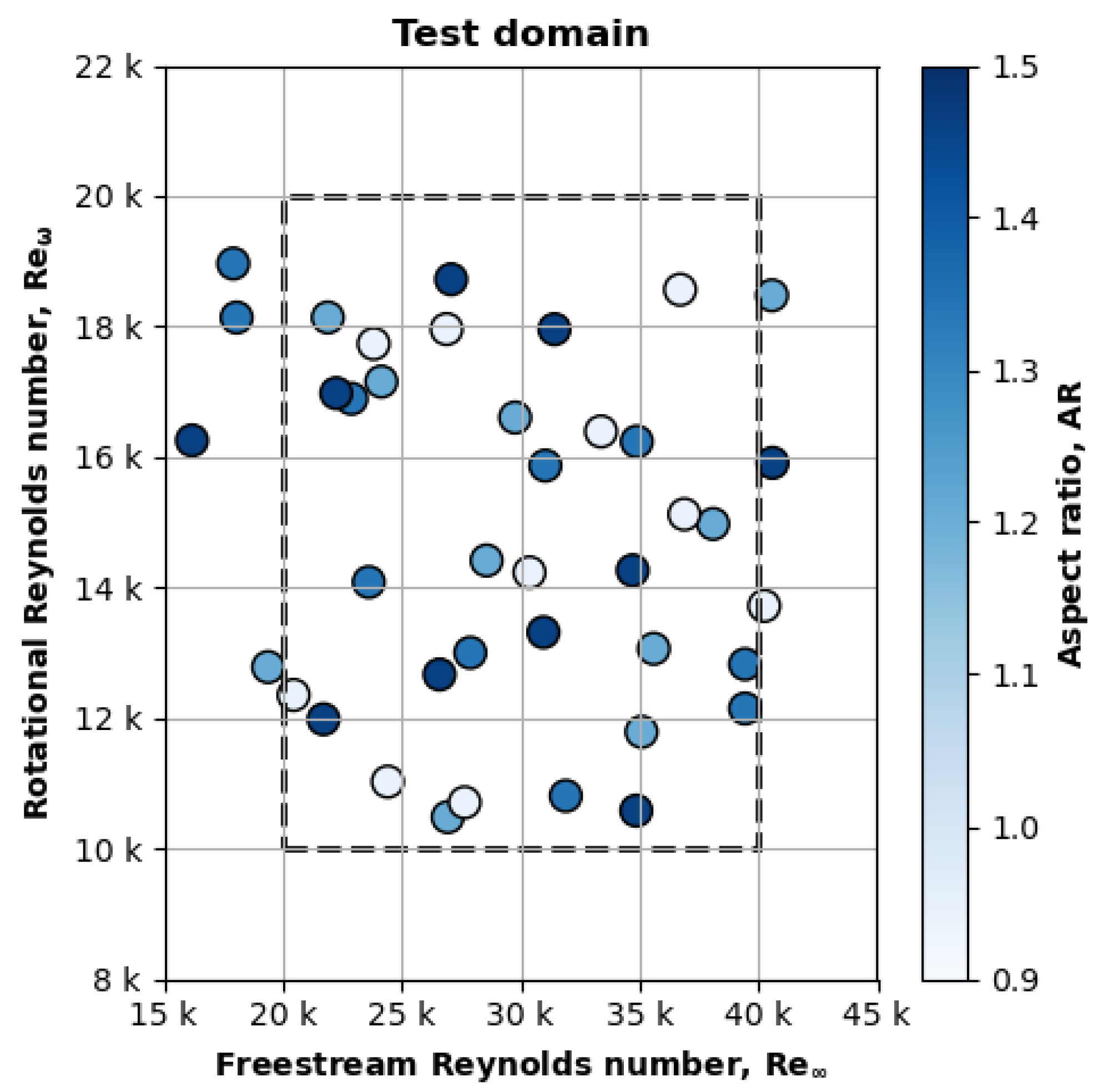
Figure 9.
The test cases with a high freestream Reynolds number and a low rotational Reynolds number exhibited relatively high uncertainty for the Nusselt number measurement.
Figure 9.
The test cases with a high freestream Reynolds number and a low rotational Reynolds number exhibited relatively high uncertainty for the Nusselt number measurement.

Figure 10.
A filter removed 18 test cases with high relative Nusselt uncertainty.

Figure 11.
The Nusselt number of the remaining 22/40 low-uncertainty cases.

Figure 12.
The proposed model captures the dip in Nusselt number at = 18,000.

Figure 13.
The proposed model captures the concave experimental trend.

Figure 14.
The proposed model captures the minimum near 5800 min−1 and the overall trend better than the other models.
Figure 14.
The proposed model captures the minimum near 5800 min−1 and the overall trend better than the other models.

Figure 15.
Heat transfer coefficient vs. freestream velocity.

Figure 16.
The literature models over-predict temperature by many orders of magnitude.

Figure 17.
Our model predicts temperature within 10 K of measured values.

Figure 18.
Efficiency–thermal model integration.

Figure 19.
Motor efficiency increases strongly with rotational speed.

Figure 20.
The motor’s limit torque at 3000 min−1 decreases by 25% in the hot environment.


Table 1.
The salient specifications of the tested motors.
| Motor | 1 | 2 | 3 | 4 | ||
|---|---|---|---|---|---|---|
| Diameter | D | [mm] | 48 | 60 | 42 | 42 |
| Length | L | [mm] | 36 | 41 | 35 | 45 |
| Lateral surface area | [cm2] | 55 | 77 | 46 | 60 | |
| Aspect ratio | 1.3 | 1.5 | 1.2 | 0.9 | ||
| Full specifications | Ref. [36] | Ref. [37] | Ref. [38] | Ref. [39] |
Table 2.
Sensor uncertainties.
| Torque | 0.4 N·mm | |
| Rotational speed | 2 rad/s | |
| Electric power | 0.5 W | |
| Temperature differential | 1 K |
Table 3.
Salient motor specifications.
| Torque constant | 20.5 N·mm/A | |
| Winding resistance | 52 m | |
| No-load current | 0.7 A | |
| DC voltage | 16 V | |
| Diameter | D | 48.2 mm |
| Length | L | 36.0 mm |
Disclaimer/Publisher’s Note: The statements, opinions and data contained in all publications are solely those of the individual author(s) and contributor(s) and not of MDPI and/or the editor(s). MDPI and/or the editor(s) disclaim responsibility for any injury to people or property resulting from any ideas, methods, instructions or products referred to in the content. |
© 2024 by the authors. Licensee MDPI, Basel, Switzerland. This article is an open access article distributed under the terms and conditions of the Creative Commons Attribution (CC BY) license (https://creativecommons.org/licenses/by/4.0/).
Share and Cite
MDPI and ACS Style
Saemi, F.; Whitson, A.; Benedict, M. Heat Transfer Models and Measurements of Brushless DC Motors for Small UASs. Aerospace 2024, 11, 401. https://doi.org/10.3390/aerospace11050401
AMA Style
Saemi F, Whitson A, Benedict M. Heat Transfer Models and Measurements of Brushless DC Motors for Small UASs. Aerospace. 2024; 11(5):401. https://doi.org/10.3390/aerospace11050401
Chicago/Turabian StyleSaemi, Farid, Annalaine Whitson, and Moble Benedict. 2024. "Heat Transfer Models and Measurements of Brushless DC Motors for Small UASs" Aerospace 11, no. 5: 401. https://doi.org/10.3390/aerospace11050401
Note that from the first issue of 2016, this journal uses article numbers instead of page numbers. See further details here.