
Large-Eddy vs. Reynolds-Averaged Navier–Stokes Simulations of Flow and Heat Transfer in a U-Duct with Unsteady Flow Separation †
School of Aeronautics and Astronautics, Purdue University, West Lafayette, IN 47907, USA
*
Author to whom correspondence should be addressed.
†
This paper is an extended version of our paper published in 2018 Joint Propulsion Conference, Cincinnati, OH, USA, 9–11 July 2018.
‡
Current address: Virgin Galactic Holdings, Inc., Las Cruces, NM 88011, USA.
Energies 2024, 17(10), 2414; https://doi.org/10.3390/en17102414
Submission received: 14 April 2024
/
Revised: 11 May 2024
/
Accepted: 13 May 2024
/
Published: 17 May 2024
(This article belongs to the Special Issue High-Performance Numerical Simulation in Heat Transfer)
Abstract
:Large-eddy simulation (LES) and Reynolds-Averaged Navier–Stokes (RANS) equations were used to study incompressible flow and heat transfer in a U-duct with a high-aspect-ratio trapezoidal cross section. For the LES, the WALE subgrid-scale model was employed, and its inflow boundary condition was provided by a concurrent LES of incompressible fully-developed flow in a straight duct with the same cross section and flow conditions as the U-duct. LES results are presented for turbulent kinetic energy, Reynolds stresses, pressure–strain rate, turbulent diffusion, turbulent transport, and velocity–temperature correlations, with a focus on how they are affected by the U-turn region of the U-duct. The LES results were also used to assess three commonly used RANS models: the realizable k-ε with the two-layer model in the near-wall region, the two-equation shear-stress transport model, and the seven-equation stress-omega Reynolds stress model. Results obtained show steady and unsteady RANS to incorrectly predict the effects of unsteady flow separation. The results obtained also identified the terms in the RANS models that need to be modified and suggested how turbulent diffusion should be modeled when there is unsteady flow separation.
1. Introduction
The turbine component of advanced gas turbines operates at high temperatures for increased thermal efficiency. Thus, it must be cooled to maintain its material’s structural integrity for reliable operation. Tremendous advances have been made in developing efficient and effective cooling methods; see, e.g., [1,2,3,4,5,6,7,8]. Further advances require a deeper understanding of the cooling processes.
High fidelity physics-based design tools such as computational fluid dynamics (CFD) could provide the understanding needed. Though direct numerical simulation (DNS) and large-eddy simulation (LES) have the potential to provide the accuracy needed, they are computationally intensive and not yet practical for use in the design and analysis of the very high Reynolds-number flows involved in turbine cooling [2,6,9]. CFD based on the Reynolds-Averaged Navier–Stokes (RANS) equations—albeit less accurate—is the most widely used because it is computationally much less demanding [1,2,3,4,5,6,7].
Considerable research has been conducted to improve the accuracy of RANS models [10,11,12,13,14,15,16,17]. The inaccuracy of RANS arises because RANS averages all length scales from the largest to the smallest, and the large scales depend on the geometry and the operating conditions of the problem studied. Since different problems have different geometries and operating conditions, no RANS model can be universal (i.e., applicable to every geometry and operating condition). As a result, benchmark-quality data generated by DNS that resolves all scales from integral to Kolmogorov and those by LES from integral to Taylor are useful to guide the development of RANS models for flows with similar geometries and operating conditions. Thus, Parneix et al. [18] showed terms in RANS models could be substituted with LES or DNS data to improve accuracy. Zhang and Shih [19,20] showed how upstream LES data could be used to adaptively modify the downstream RANS model so that RANS could be nearly as accurate as LES for the problem being studied. Basically, different sets of benchmark data are needed for different classes of geometries and flow conditions.
One geometry of interest in turbine cooling is the U-duct [1,2,3,4,5,6,7,8,9]. Most CFD studies of flow and heat transfer in U-ducts are based on RANS (see, e.g., [21,22,23,24,25,26,27,28,29,30,31,32,33] and the references cited there). Relatively few have performed LES on U-ducts. Métais and Salinas-Vázquez [34] used LES to analyze the turbulent flow through a heated straight square duct. Hebrard et al. [35] and Munch [36] used LES to study a heated curved-square duct. Guleren and Turan [37] and Acharya and Tyagi [38] performed an LES study of a rotating duct. Laskowski and Durbin [39] performed DNS of flow and heat transfer in a stationary and rotating U-duct. Hu and Shih [40] performed an LES study of a U-duct with a trapezoidal cross section that matched well with experimental data and showed RANS to provide reasonably accurate results in the U-duct’s up-leg but not in the down-leg. Though that study performed a very detailed verification and validation study, it did not provide the turbulent statistics from the LES study. Those statistics are needed to guide the development of RANS models for U-ducts.
The objective of this study is twofold. The first is to provide benchmark LES data that can be used to guide the development of RANS models for predicting flow and heat transfer in U-ducts that include results for the mean flow and the Reynolds stresses as well as the pressure–strain rate, turbulent diffusion, turbulent transport, and velocity–temperature correlations. Second, use the data generated to assess the performance of the following three widely used RANS models: (1) the realizable k-ε model [41]; (2) the shear-stress transport model (SST) [15,42,43,44]; and (3) the stress-omega Reynolds stress model (RSM) [15].
The organization of this paper is as follows: First, the U-duct problem studied is described. Next, the governing equations used for RANS and LES are given. Afterwards, the numerical methods used to generate solutions, the grid-sensitivity study, and the validation study are presented. This is followed by the results generated and a summary of key findings.
2. Problem Description
The U-duct with a high-aspect-ratio trapezoidal cross section selected for study is shown in Figure 1. This configuration was chosen for the following three reasons: The first is that there is experimental data that can be used to validate the LES [32]. Second, U-ducts with trapezoidal cross sections induce more complicated turbulent flows than those with circular, square, or rectangular cross sections, so that the turbulent statistics generated could guide the development of RANS models for a more general class of U-ducts. Third, U-ducts with trapezoidal cross sections are relevant to turbine cooling.
The U-duct with a trapezoidal cross-section studied experimentally and reported in Ref. [32] is shown in Figure 1. Its dimensions are H1 = 11.72 mm, H2 = 28.48 mm, W1 = 54.24 mm, W2 = 114.83 mm, L1 = 246 mm, L2 = 192 mm, and d = 6.35 mm, with a hydraulic diameter of Dh = 29.04 mm. In the experimental study [32], the flow entering the U-duct was “fully” developed.
To simulate the experimental study for the U-duct shown in Figure 1, two configurations were used as shown in Figure 2, one for RANS and one for LES. The configuration used for RANS (Figure 2a) has a duct of length Li = 40Dh with the same cross section as the U-duct appended to the up-leg of the U-duct to ensure that the flow entering the U-duct is “fully” developed. To ensure that there is no reverse flow at the exit of the U-duct, another straight duct of length LE = 384 mm with the same cross section as the U-duct was appended to the down-leg of the U-duct. For this U-duct with its appended ducts, air enters with uniform velocity Vin = 12.65 m/s and uniform temperature Tin = 343.15 K. All wall temperatures were maintained at Twall = 313.15 K, and the static pressure at the duct’s exit was maintained at Pb = 1 atm.
For the configuration used for LES (Figure 2b), the up-leg portion of the U-duct shown in Figure 1 was shortened by 96 mm to reduce computational cost. The inlet of the resulting U-duct is still sufficiently upstream of the bend and unaffected by the turn region. To obtain a fully-developed flow at the inlet of the “shortened” U-duct, the boundary conditions imposed there were provided by a concurrent LES of incompressible fully-developed flow in a straight duct, where the temperature at its inlet is adjusted so that the bulk temperature is the same as the RANS simulations at that same location. All other boundary conditions used for LES are the same as those described for the RANS configuration. Additional details of the problem studied are given in Refs. [32,40].
3. Formulation
For the two configurations of the U-duct studied (shown in Figure 2), the flow is assumed to be incompressible. The incompressible-flow assumption is reasonable because the Mach number is much less than 0.3 throughout the U-duct, so density changes due to speed changes are small. Also, Twall − Tin and the pressure drop along the U-duct from its inlet to its outlet are small, so the density change due to changes in temperature and pressure is small as well. In addition, since Twall − Tin is small, all thermodynamics and transport properties were taken to be constants and evaluated at T = (Tin + Twall)/2. Viscous dissipation was neglected as well, since the Eckert number for this problem is small.
3.1. Governing Equations for RANS
The governing equations used for the RANS simulations are the Reynold-averaged continuity, momentum (Navier–Stokes), and thermal-energy equations for incompressible flow, and they are as follows [15,16]:
In the above equations, an overbar denotes an ensemble-averaged quantity; are the Reynolds stresses; is the fluctuating component of the instantaneous velocity in the direction; and is the temperature fluctuation about the mean temperature. For statistical stationary turbulent flows, ensemble to close Equations (1) to (3), models are needed for and . In this study, three RANS models were examined. Two are eddy-viscosity models: the realizable k-ε model [41] and the shear-stress transport (SST) [15,42,43,44]. The third model is the stress-omega Reynolds stress model (RSM) [15].
3.1.1. Eddy-Viscosity Model
For the two eddy-viscosity models examined, the Reynolds stresses are given by the following equation:
where , , and are the turbulent kinetic energy, mean strain-rate tensor, and eddy viscosity, respectively. The realizable k-ε and the SST models differ in how is modeled.
In the above equations, , , , , and with recovering the standard value of 0.09 in the fully turbulent region of the flow. Since the realizable k-ε is not valid in the near-wall region, where the turbulent number based on turbulent kinetic energy is small, the one-equation model of.
The turbulent kinetic energy, k, and its dissipation rate, , in Equation (5) are obtained by the following transport equations:
where represents the generation of turbulent kinetic energy due to the mean velocity gradients; = 1.9; and and are the turbulent Prandtl numbers for and , respectively.
Since the realizeable k-ε model given by Equations (9) and (10) is not valid in the near-wall region, the one-equation, two-layer model of Chen–Patel was used there [45]. Thus, though the realizeable k-ε model is a two-equation model, the turbulence model used in the near-wall region is a one-equation model.
Though the realizeable k-ε model is not valid in the near-wall region, the k-ω model is. Thus, the k-ω model offers the benefit of a two-equation model for the entire turbulent flowfield. However, the k-ω model is sensitive to freestream turbulence. The SST model overcomes the challenges of the k-ε and k-ω models by using the k-ε model away from the walls where the flow is fully turbulent and the k-ω model in the near-wall region. The switch between these two equations is carried out by a smooth interpolation [9].
For the SST model, in Equation (4) is modeled by the following [15,42,43,44]:
where is the magnitude of the strain rate and
The model constants in the above equations are as follows: , , . For the SST model, the turbulent kinetic energy, k, and its specific dissipation rate, , are obtained by the following:
In Equations (14) and (15), represents the generation of turbulence kinetic energy, and represents the generation of . and are the turbulent Prandtl numbers for and , respectively.
3.1.2. Reynolds Stress Model
For the stress-omega Reynolds stress model, there is a transport equation for each of the six Reynolds stresses, . These transport equations are given by the following [15,46]:
Of the terms in the above six equations, convection, production, and viscous diffusion do not require modeling. Turbulent diffusion, pressure strain, and dissipation tensors, however, do need to be modeled. The turbulent-diffusion term in Equation (16) is modeled by generalizing gradient-diffusion as shown below.
where the eddy viscosity, , is given by the following:
with being computed by using Equation (15).
The dissipation tensor in Equation (16) is modeled by the following:
where is computed by using Equation (10).
For the pressure–strain rate in Equation (16), the classical approach uses the following decomposition:
where is the slow pressure–strain term; is the rapid pressure–strain term; and is the wall reflection term. In the stress-omega Reynolds stress model, the wall-reflection term is neglected, and the other two terms are approximated by the LRR model [15] as shown below.
where , , , , , and
The stress-omega Reynolds stress model given by Equations (6) to (22) is valid in the near-wall region as well as the fully turbulent region of the flowfield.
3.2. Governing Equations for Large-Eddy Simulation
In LES, large scales of the turbulent flow—which depend strongly on the geometry and boundary conditions—are simulated, and the smaller scales—which have more universal properties because the cascading process diminishes the effects of the flow’s history—are modeled in terms of the simulated larger scales. The governing equations used in LES are obtained by applying a spatial filter to the unsteady, three-dimensional form of continuity, momentum (Navier–Stokes), and thermal energy equations, yielding the following [15]:
In the above equations, the hat above a variable indicates a filtered variable, and is the subgrid-scale stresses. To close the filtered equations, must be modeled, and one approach is to employ an eddy viscosity model such as
where is the sub-grid scale turbulent viscosity. Many models have been proposed for . In this study, the wall-adapting Local eddy viscosity model (WALE) formulated by Nicoud and Ducros [47] was used, and it is given by the following:
where = 0.325; is the cutoff width (which is connected to the grid spacing employed in the numerical solution); and
One advantage of the WALE model is that damping is not needed near the wall. It naturally goes to zero at the wall and reproduces the proper scaling of . Also, it is sensitive to both the strain and rotation rate of the small structures.
3.3. Eddy Diffusivity Hypothesis (EDH)
Thus far, only the models for the Reynolds stresses in RANS and the subgrid-scale stresses in LES are given. In the energy equation given by Equation (3) for RANS and Equation (25) for LES, the correlation between velocity and temperature fluctuations also needs to be modeled. In this study, the eddy-diffusivity concept was invoked as follows:
In Equation (29), the bar denotes Reynolds averaging if RANS and spatially filtering if LES, and is the eddy-diffusivity of thermal energy. The Reynolds analogy between heat and momentum transport suggests that is closely related to the eddy or subgrid-scale viscosity so that
where is the turbulent Prandtl number. In this study, is taken to be 0.85 for both RANS and LES.
4. Numerical Method of Solution
GAMBIT was used to generate the grids used in this study, and version 16.2.0 of the Fluent UNS code [48] was used to generate all of the solutions.
For RANS, the SIMPLE algorithm was used [49]. The advection terms in the momentum, energy, and turbulent transport equations were approximated by second-order upwind formulas, and terms in the pressure equation were approximated by second-order central formulas. Since the SIMPLE algorithm is an iterative method and only steady-state solutions were of interest, iterations were continued until residuals for all equations plateaued to ensure convergence to steady state. At convergence, the scaled residual is always less than 10−5 for the three components of the velocity, less than 10−7 for the energy equation, less than 10−4 for turbulent quantities, and less than 10−3 for the continuity equation.
For LES, the SIMPLE algorithm was also used. The time derivatives were approximated by the bounded second-order implicit scheme. The time-step size used ensured the maximum CFL number to be less than 0.6, which was small enough to resolve the Taylor time scale, and ten sub-iterations were found to be sufficient for the solution to converge at each time step. On spatial derivatives, second-order central differencing was used. Note that when the filter width used is variable because the grid spacing used is what determines the filter width, assuming the LES spatial filter and the differential operators are commutative as implied in Equations (23) to (25) limits the order of time and spatial accuracy to two. When solving the pressure equation, the PRESTO scheme was employed, as suggested by Lampitella [50].
Figure 3 shows the grid employed for RANS and LES. It is a multi-block structured grid with a wrap-around O-H grid about the walls of the U-duct and an H-H grid in the duct’s core. As can be seen in Figure 3, the grid points were clustered on all solid surfaces, and a wrap-around grid was employed. Also, the of the first grid point next to all walls is less than unity, so the integration of turbulence models extends all the way to the wall. Also, there were 4 to 5 cells within a of 5. For RANS, the grid used had 4,129,920 cells. The grid employed was obtained via a grid-sensitivity study, and the details are given in Ref. [32].
The grid used for LES has 16,110,000 cells. In addition to for the first grid point next to all walls, the spacing between grid points for the O-H grid was in the streamwise direction, normal to the wall, and in the spanwise direction. For the H-H grid, in the streamwise direction and and between 1 and 10. The grid used was obtained by examining the following criteria: clustering of the cell’s growth ratio normal to the wall, spanwise cell aspect ratio, streamwise cell aspect ratio, and enough cells to resolve the energy-cascade process in the inertial subrange everywhere in the duct (i.e., capture the Kolmogorov −5/3 law). In addition, the Celik criterion is given by the following equation:
where denotes the effective subgrid viscosity and denotes the laminar kinematic viscosity [51], where LES_IQ should be greater than 0.8 for good LES predictions. The grid used had LES quality indexes greater than 0.9 everywhere. Details of the grid-sensitivity study performed for LES are given in Ref. [40].
5. Results
In this section, the results obtained by RANS and LES for the U-duct problem studied are presented. First, the heat-transfer coefficient obtained is compared with experimentally measured values, which serves as a validation of the RANS and LES results. Afterwards, the turbulent kinetic energy and Reynolds stresses predicted by the RANS models and LES are compared. Next, the pressure–strain rate, pressure diffusion, and turbulent transport obtained by the Reynolds stress model are compared with those from LES. This is followed by an assessment of the predictive capability of models for velocity–temperature correlations.
5.1. Heat-Transfer Coefficient
Figure 4 and Figure 5 show the heat-transfer coefficient (HTC) obtained by RANS, LES, and experimental measurements (EXP), where the experimental data are from Ref. [32] and where the procedure used to obtain the bulk temperature to compute the HTC for RANS and LES is the same as that used in the experimental study described in Ref. [32]. Figure 4 shows contours of the HTC, and Figure 5 shows a more quantitative comparison of the HTC distribution about the turn region, which starts at X/L1 = 7.4 in the up-leg and ends at X/L1 = 7.4 on the down-leg.
In the up-leg, though only RSM and LES could account for the effects of the corner vortices, Figure 4 and Figure 5 show all models except k-ε to match EXP well. Though k-ε could not accurately predict the distribution of the HTC in the up-leg (see X/L1 = 0.33, 0.5, and 0.65 in Figure 5), all models including k-ε predicted regionally averaged HTCs well, where the maximum errors relative to EXP were less than 2.5% for all models. In the turn region, the HTC is increased because of the impingement of the cooling flow on the wall at X/L1 = 1 and Dean-type secondary flow that brings cooler fluid from the duct’s core to the wall. In this region, only LES could predict the flow features and their effects on heat transfer correctly. The maximum relative errors in the predicted regionally averaged HTCs were 14.5% for RSM, 29% for SST, and 50% for k-ε. The biggest and most important difference between RANS and LES occurs in the down-leg, where all RANS models predicted a region of low HTC about the bend. This is because all RANS models predicted a large, separated region about the bend that starts at the tip of the wall that separates the up-leg and the down-leg of the U-duct. Such a low region of HTC was not observed in the experimental measurements (EXP). LES, however, was able to predict the experimentally measured HTC correctly. It did so because the separation at the tip of the separator at X/L1 = 7.4 was found to be unsteady, with the separation bubble shedding periodically. By predicting a large, separated region about the bend, all RANS models overpredicted the HTC next to the outer wall in the down-leg of the U-duct, whereas LES slightly underpredicted the HTC in that region. Though none of the RANS models were able to predict the HTC distributions, Hu et al. [40] showed the SST and RSM models to predict average HTC reasonably well. In the down-leg part after the turn region, the maximum relative error in the averaged HTC was 10%. Thus, if only averages are needed, then SST and RSM may be adequate.
Once it was recognized that the separation that takes place at the leading edge of the separator is unsteady, unsteady RANS (URANS) was performed, where perturbations were introduced at and about the separator tip to induce unsteadiness. In all cases, once the perturbations were no longer applied, unsteady separation could not be sustained by URANS, and the flow became steady and identical to that predicted by steady RANS. Thus, the unsteady separations that occur at the tip of the separator are induced by unsteadiness in the turbulent flow field and not by asymmetry in geometry or boundary conditions, such as the unsteady separations that take place for flows past blunt objects such as cylinders and cubes.
On the flow field predicted by LES, the magnitude of the instantaneous velocity in the “geometric” symmetry plane at Y = 0 is shown at the top of Figure 6. To examine the frequencies of the shedding in the LES solution, a probe marked as ⊕ is inserted to record the x-velocity as a function of time. The discrete Fourier transform was then used to convert the data to the frequency domain, which is shown at the bottom of Figure 6. In this figure, the peak values—2.86 Hz, 7.14 Hz, and 12.86 Hz—are the frequencies created by the unsteady separation. The peak value of 40 Hz corresponds to the frequency of the dominant energy-carrying turbulent structures. Based on the frequency of 40 Hz and the total averaging time of the calculation, about 28 vortices are passed by during the simulation (Appendix A).
5.2. Turbulent Kinetic Energy and Reynolds Stresses
Figure 7 shows the turbulent kinetic energy (TKE) predicted by RANS and LES in planes located at X/L1 = 0.16, 0.33, 0.5, 0.65, turn, 0.8, and 0.9. From this figure, it can be seen that all RANS models are able to predict TKE in the up-leg but significantly underpredict TKE in the turn region and in the down-leg. RANS predicted a large, separated region in the down-leg; RANS underpredicted TKE in the separated region and overpredicted TKE for the flow that was constricted and hence accelerated by the separated region. LES showed a high TKE next to the separator because of the unsteady separation at its tip and the passage of separated vortices over its surface.
Figure 8 shows the six components of the Reynolds stresses, normalized by the mean friction velocity in several planes. Since the domain in the RANS simulations only included a symmetric half of the U-duct, the other half plotted in Figure 8 is mirrored without any correction to the sign of the values. For the normal components of the Reynolds stresses, predictions by RANS models show that has about 50% higher than the other two normal components when the peak values of all three normal components are all at similar locations in each plane. For LES, the peak values of the three normal components are comparable. In the down-leg, dominates the shear layer between the main flow and the separation bubble, while dominates the core of the main flow and dominates the near wall region.
For the shear components of the Reynolds stresses, dominates in the turn region (X/L1 = 0.9) for k-e and SST, while three shear components have similar values for RSM and dominates for LES. In the sharp corner near the separator tip (X/L1 = turn), similar to the normal components, high values are obtained by LES, while lower peak values and a shifted location far away from the separator tip are obtained by RANS models. The contours of X/L1 = 0.65 can be considered the continuation of the contours of X/L1 = turn. At X/L1 = 0.33, a high-value area of near the inner wall is obtained by RSM, which does not exist in LES prediction. On the other hand, RSM is the only RANS model that is not able to predict LES results.
5.3. Pressure Strain Rate, Pressure Diffusion, and Turbulent Transport
For the RSM model, the terms that are the most challenging to model are the pressure–strain rate, pressure diffusion, and turbulent transport. Thus, it is of interest to understand if LES could provide guidance in modeling those terms for this U-duct problem. In this section, pressure–strain rate, pressure diffusion, and turbulent transport based on the exact equations and their models are compared by using data from RSM and from LES at locations shown on the left of Figure 7 to understand where model improvements are needed. This section also compares pressure diffusion with turbulent transport and pressure diffusion with pressure–strain rate based on their exact equations by using LES data to understand their relative importance.
Figure 9 shows the six components of the pressure–strain rate in the turn region at X/L1 = turn, where the flow is the most complicated. For each of the six components, three values are given. One is based on the RSM model using RSM data (denoted as RSM (RSM data)); the second is based on the RSM model using LES data (denoted as RSM (LES data)); and the third is based on the exact definitions of the pressure–strain rate with LES data (denoted as Exact (LES data)).
Comparing RSM (LES data) and Exact (LES data) shows the model for pressure–strain rate used in RANS is reasonable, with the maximum relative error less than 20%. However, when RSM (RSM data) is compared with RSM (LES data), the relative error is quite large. This indicates that there are errors in the RSM data but not in modeling the pressure–strain rate.
From Figure 9, the following observations can be made: The pressure–strain rate is significantly under-predicted by using the data from RSM. If LES data are used, then the modeled pressure–strain tensors are higher near the sharp corners and near the top and bottom walls. By comparing RSM (LES data) with Exact (LES data), the shear components can be seen to compare well except Π23 in the region near the top and bottom walls but away from the inner wall. However, the normal components are less accurately predicted. This is because the normal components involve TKE, which was underpredicted, which in turn causes incorrect prediction of the pressure strain in a circuitous manner.
Comparing RSM (RSM data), RSM (LES data), and Exact (LES data) shows the pressure–strain model proposed by Launder [52] and Wilcox [15] to be quite reasonable qualitatively. Quantitatively, some adjustments are still needed, especially for the normal components in connection with TKE.
The pressure–diffusion term (Dp) is usually modeled together with the turbulent transport term (TT), and those two terms are collectively called turbulent diffusion (DT) [53]. The turbulent diffusion is typically modeled via gradient diffusion—a very simple model for a very complex process. Figure 10 shows the RSM model for turbulent diffusion tensors calculated by RSM and LES data in the middle of three planes located at X/L1 = 0.65, 0.8, and 0.9. From this figure, RSM data can be seen to follow the trend of LES data in most of the domain, except around the second corner of the separator (Z/W1 ~ 0 at X/L1 = 0.8). Only the trend of DT,12 is well predicted by RSM data at that location. Nevertheless, the value of turbulent diffusion predicted by the RSM data is about 0.5% of the LES data. If the RSM model of turbulent diffusion with LES data is compared with the turbulent diffusion calculated by LES data with its exact definition, then Figure 11 shows that the error is quite large. The RSM model of turbulent diffusion with RSM data is 105, which is smaller than the value that it should be.
To understand the contribution of pressure diffusion (Dp) and turbulent transport (TT) in turbulent diffusion (DT), Dp and TT were calculated by using the exact definition with LES data and compared with each other at different locations as shown in Figure 12, Figure 13 and Figure 14. The validation and verification of the pressure–diffusion calculations are given in Appendix B. From these figures, it can be seen that Dp and TT differ in sign, magnitude, and trend. On magnitude, pressure diffusion is at least 104 times higher than turbulent transport at all the locations examined. This indicates pressure diffusion dominates in the modeling of turbulent diffusion. Thus, when modeling turbulent diffusion, one only needs to model pressure diffusion. By comparing Figure 10 and Figure 11 with Figure 12, Figure 13 and Figure 14, it can be seen that existing models for turbulent diffusion are orders of magnitude smaller than what they should be. This is because existing models only model turbulent transport when they should have been modeling pressure diffusion.
Mansour et al. [53] proposed pressure–strain rate (Π) and pressure diffusion (DP) given by Equations (16) to (20) to be modeled together because the two terms presented below have opposite signs and tend to cancel each other near wall boundaries.
To examine this assertion, Figure 15 compares each of the six components of Πij and DP,ij based on their exact definitions given above by using LES data. In Figure 15, pressure–strain rates are shown on the top half of each of the trapezoidal cross sections and pressure diffusion on the bottom half. The legends are similarly arranged. From this figure, it can be seen that for the problem studied, the difference between Πij and DP,ij can be as high as 105. At the tip of the separator, where unsteady separation starts, Dij can be from 10,000 to 100,000 times larger than Πij. In the down-leg, where separated flows move downstream, DP,ij is about 50,000 times larger than Πij. Though the magnitudes differ considerably, Πij and DP,ij have similar qualitative features, including their signs, especially in the down-leg. The enormous difference between Πij and DP,ij in the down-leg shows that Mansour et al.’s assertion is not always true.
The questions now are as follows: What does DP,ij >> Πij mean? When DP,ij >> Πij, which occurs in the down-leg of the U-duct, Reynolds stresses will diffuse at a much higher rate from the outer wall, where it is high, toward the inner wall, where it is lower. This diffusion is so large that it causes the local flow to behave as if its Reynolds number is near unity. Flows with such low Reynolds numbers can turn corners without separation, which is why unsteady separation appears after time averaging. Thus, when there are unsteady separations, modeling pressure diffusion is as important as modeling pressure–strain rate. As shown in Figure 10 and Figure 11, the RSM model developed by Wilcox does have the potential to predict larger values of the pressure–diffusion tensor, albeit not yet implemented to sense and account for unsteady separation. Basically, when there is unsteady flow separation, turbulent diffusion must be made high enough to enable the mean flow to turn a corner with a minimal-sized separation bubble.
5.4. Eddy Diffusivity Hypothesis
The models for the velocity–temperature correlations—, , and —in the thermal energy equation computed by k-ε, SST, and RSM are compared with those from the time-averaged LES solution in Figure 16 at several locations. From this figure, it can be seen that and are predicted fairly accurately in the up-leg (X/L1 = 0.65 and 0.8 and Z/W1 > 0), but not , where all RANS models studied predicted almost identical results that differ considerably from those from LES. In the turn region (X/L1 = 0.9), the trends for , , and are roughly captured by the RANS models, but the magnitudes are off by a factor up to five. In the down-leg (X/L1 = 0.8 and 0.65 and Z/W1 < 0), k-ε predicted trends most similar to LES. For SST and RSM, not only are the trends predicted incorrectly when compared to LES, but even the signs of the values are different. Though the comparison with LES improves at X/L1 = 0.65, SST and RSM predict two peaks, while only one is predicted by k-ε and LES.
Figure 17, Figure 18 and Figure 19 show the temperature gradients predicted by RANS and LES. In the up-leg, all RANS models and LES yielded similar results for . However, the inability of k-ε and SST to predict secondary flows in the four corners of the trapezoidal duct creates noticeable errors for both and . RSM, on the other hand, is able to predict those secondary flows, so better matches are predicted by LES near the inner wall; they nearly perfectly match at the center of the duct, but are still less accurate near the outer wall. A common error made by all RANS models is the prediction of in the near wall region, where LES data show a small area of positive value while no RANS model is able to capture that.
Since secondary flows cannot be predicted by RANS models with scalar eddy viscosity, this is one source of the errors for the k-ε and SST models. Though RSM could predict corner secondary flows, Figure 20 shows LES to predict more turbulent mixing about the corners by the secondary flows than by RSM. In the corners of both the inner and outer walls, smaller and weaker corner vortices are predicted by RSM closer to the corners, so that the convex contour lines of low temperature as shown by LES do not appear in the prediction of RSM, resulting in an error of near the walls in the straight duct. To improve that, more efforts to accurately approach ,, and via RSM have to be made.
Temperature gradients predicted are also affected by how turbulent thermal diffusivity, , is modeled. In this study, is modeled by the turbulent Prandtl number, , namely,
where is connected to turbulent eddy viscosity, , and computed by the k-ε, SST, and RSM models. Although varies somewhat, it is taken to be a constant with a value of 0.85, i.e.,
To evaluate Equations (31) and (32), LES data are used to calculate the turbulent thermal diffusivity. Since there are three velocity–temperature fluctuation correlations and three mean temperature gradients but only one turbulent thermal diffusivity in the RANS models, the least squares method is applied to the following equation:
The comparison of the turbulent Prandtl number between Equations (32) and (33) is plotted in Figure 21. The RANS models used are fairly accurate in the up-leg, where the maximum relative error in the averaged heat-transfer coefficient is 2.5%. In the turn region, the maximum relative error is 14.5% for RSM-τω, 29% for SST, and 50% for k-ε and RSM-LPS.
But LES data shows some extreme values around the tip of the separator, where strong shear force occurs, and near the inner wall of the down-leg, both before and after the reattachment of the separation flow. The calculated turbulent Prandtl number ranged from −15 to 15 in the shear layer between the separation flow and the main flow, from −3 to 15 near the inner wall before the reattachment, and from −20 to 3 near the inner wall after the reattachment.
6. Conclusions
Large-eddy simulations (LES) show k-ε, SST, and RSM models to be inadequate in predicting the flow and heat transfer in the turn and down-leg regions of the U-duct because they were unable to predict the unsteady flow separation about the separator that was induced and sustained by turbulent fluctuations and not by geometry or asymmetry. Also, k-ε and SST could not predict any of the Reynolds stresses correctly in the turn region and in the down-leg of the U-duct. For RSM, the modeling of the pressure–strain rate was found to match LES data well, both qualitatively and quantitatively. On turbulent diffusion, the exact correlations based on LES data can be up to five orders of magnitude higher than those predicted by RSM. This huge error indicates that the two terms in turbulent diffusion—turbulent transport and pressure diffusion—should be modeled separately. LES data show turbulent transport to be ignorable throughout the entire domain. Thus, the focus should be on modeling pressure diffusion. In particular, when there is unsteady separation, turbulent diffusion should be orders of magnitude higher so that the mean flow can turn a corner with a minimum-sized separation bubble. On the velocity–temperature correlations, only is reasonably well-predicted, but not and , not even qualitatively. The eddy-diffusivity model for the velocity–temperature correlations was found to be an extreme simplification because the turbulent Prandtl number is clearly not a constant and varies appreciably. The LES data could be used to guide the development of a better model for these terms.
Author Contributions
Conceptualization, K.S.H. and T.I.-P.S.; Methodology, K.S.H. and T.I.-P.S.; Validation, K.S.H.; Formal analysis, K.S.H. and T.I.-P.S.; Investigation, K.S.H.; Data curation, K.S.H.; Writing—original draft, K.S.H. and T.I.-P.S.; Writing—review & editing, K.S.H. and T.I.-P.S.; Visualization, K.S.H.; Supervision, T.I.-P.S.; Funding acquisition, T.I.-P.S. All authors have read and agreed to the published version of the manuscript.
Funding
This work was supported by the Ames Laboratory and the National Energy Technology Laboratory with funding from the Department of Energy under Contract No. DE-AC02-07CH11358/Agreement No. 26110-AMES-CMI. The authors are grateful for this support.
Data Availability Statement
The original contributions presented in the study are included in the article, further inquiries can be directed to the corresponding author.
Acknowledgments
The authors are grateful to Mark Bryden and John Crane for the discussions on the research and results.
Conflicts of Interest
Author Kenny S. Hu employed by the Virgin Galactic Holdings, Inc. The remaining author declares that the research was conducted in the absence of any commercial or financial relationships that could be construed as a potential conflict of interest.
Nomenclature
| Dh | hydraulic diameter (Dh = 4Ac/C, where Ac and C are the duct’s cross-sectional area and its perimeter) |
| h | heat-transfer coefficient |
| I | turbulent Intensity |
| k | turbulent kinetic energy |
| k | thermal conductivity |
| P | pressure |
| Prt | turbulent Prandtl number |
| q” | heat flux |
| Re | Reynolds number (Re = ρVinDh/μ) |
| T | temperature |
| Tb | bulk temperature |
| u, v, w | x, y, and z components of the velocity vector |
| uτ | friction velocity (uτ = ) |
| X, Y, Z | Cartesian coordinates for the U-duct (X is the streamwise direction) |
| nondimensional normal distance from wall = normal distance from wall) | |
| Kronecker delta | |
| dissipation rate of turbulent kinetic energy | |
| constant | |
| μ | dynamic viscosity |
| kinematic viscosity | |
| turbulent kinematic viscosity | |
| turbulent viscosity | |
| density | |
| specific turbulent dissipation |
Appendix A
For the LES of the U-duct, Figure A1 shows the history of the x-velocity and the gradient of x-velocity with their instantaneous values, “moving” time-averaged values, and the “moving” standard error. The definitions of each curve are described below.
where , is the time step size.
The mean velocity and the mean velocity gradient are averaged from t = 0.1 to 0.832. The Reynolds stresses, the velocity-pressure correlations used to analyze the pressure–strain rate and the pressure–diffusion, and the triple correlations used to analyze the turbulent transport are averaged from t = 0.3 to 0.832. In this figure, the “moving” mean values are approaching steady values and the standard errors are approaching 0, which means the time-averaged data are approaching steady state and ready to be used for analyses.
Figure A1.
Instantaneous values, time-averaged values, the standard error of the time-averaged values of the magnitude of velocity, |u|, and the velocity gradient, |, in the x-direction on the probe marked in Figure 6.
Figure A1.
Instantaneous values, time-averaged values, the standard error of the time-averaged values of the magnitude of velocity, |u|, and the velocity gradient, |, in the x-direction on the probe marked in Figure 6.

Appendix B
To validate and verify the calculation for the pressure–strain rate, the pressure diffusion, and the turbulent transport, the same processors were operated for the square straight duct simulation, and the results are shown in Figure A2a. From the figure, these three terms were in the same order of magnitude, and neither of them was obviously dominant. Three of the pressure diffusion components were compared to the DNS data provided by Huser [54] and shown in Figure A2b. According to the figure, the calculation was able to give reasonable pressure diffusion values. From Figure A2, the correctness of the pressure diffusion calculation could be ensured.
Figure A2.
Budget terms analyses for a square straight duct at the middle of the duct. (a) The pressure diffusion vs. turbulent transport vs. the pressure–strain rate. (b) The comparison of the pressure diffusion between LES data and the DNS data provided by Huser [54].
Figure A2.
Budget terms analyses for a square straight duct at the middle of the duct. (a) The pressure diffusion vs. turbulent transport vs. the pressure–strain rate. (b) The comparison of the pressure diffusion between LES data and the DNS data provided by Huser [54].

References
- Goldstein, R. (Ed.) Heat Transfer in Gas Turbine Systems; Annals of the New York Academy of Sciences: New York, NY, USA, 2001; Volume 934. [Google Scholar]
- Sundén, B.; Faghri, M. (Eds.) Heat Transfer in Gas Turbines; WIT Press: Southhampton, UK, 2001. [Google Scholar]
- Han, J.C. Fundamental Gas Turbine Heat Transfer. J. Therm. Sci. Eng. Appl. 2013, 5, 021007. [Google Scholar] [CrossRef]
- Chiu, M.; Siw, S.C. Recent Advances of Internal Cooling Techniques for Gas Turbine Airfoils. J. Therm. Sci. Eng. Appl. 2013, 5, 021008. [Google Scholar] [CrossRef]
- Ligrani, P. Heat Transfer Augmentation Technologies for Internal Cooling of Turbine Components of Gas Turbine Engines. Int. J. Rotating Mach. 2013, 2013, 275653. [Google Scholar] [CrossRef]
- Shih, T.I.-P.; Yang, V. (Eds.) Turbine Aerodynamics, Heat Transfer, Materials, and Mechanics; Progress in Astronautics and Aeronautics; American Institute of Aeronautics and Astronautics: Reston, VA, USA, 2014; Volume 243. [Google Scholar]
- Han, J.C.; Dutta, S.; Ekkad, S.V. Gas Turbine Heat Transfer and Cooling Technology; Taylor & Francis: New York, NY, USA, 2015. [Google Scholar]
- Town, J.; Straub, D.; Blak, J.; Thole, K.; Shih, T.I.-P. State-of-the-Art Cooling Technology for a Turbine Rotor Blade. ASME J. Turbomach. 2018, 140, 071007. [Google Scholar] [CrossRef]
- Tafti, D.K.; He, L.; Nagendra, K. Large Eddy Simulation for Predicting Turbulent Heat Transfer in Gas Turbines. Philos. Trans. R. Soc. A 2013, 372, 20130322. [Google Scholar] [CrossRef]
- Sarkar, A.; So, R.M.C. A Critical Evaluation of Near-Wall Two Equation Models Against Direct Numerical Simulation Data. Int. J. Heat Fluid Flow 1977, 18, 197–208. [Google Scholar] [CrossRef]
- Patel, V.C.; Rodi, W.; Scheuerer, G. Turbulence Models for Near Wall and Low-Reynolds-Number Flows: A Review. AIAA J. 1985, 23, 1308–1319. [Google Scholar] [CrossRef]
- Apsley, D.; Leschziner, M. Advanced Turbulence Modelling of Separated Flow in a Diffuser. Flow Turbul. Combust. 2000, 631, 81–112. [Google Scholar] [CrossRef]
- Wallin, S.; Johansson, A.V. An Explicit Algebraic Reynolds Stress Model for Incompressible and Compressible Turbulent Flows. J. Fluid Mech. 2000, 403, 89–132. [Google Scholar] [CrossRef]
- Pope, S.B. Turbulent Flows; Cambridge University Press: Cambridge, UK, 2000. [Google Scholar]
- Wilcox, D.C. Turbulence Modeling for CFD; DCW Industries, Inc.: La Canada, CA, USA, 1998. [Google Scholar]
- Durbin, P.A.; Shih, T.I.-P. An Overview of Turbulence Modeling. In Modelling and Simulation of Turbulent Heat Transfer; Sundén, B., Faghri, M., Eds.; WIT Press: Southhampton, UK, 2005; Chapter 1; pp. 3–31. [Google Scholar]
- Raiesi, H.; Piomelli, U.; Pollard, A. Evaluation of Turbulence Models Using Direct Numerical and Large-Eddy Simulation Data. ASME J. Fluids Eng. 2011, 133, 021203. [Google Scholar] [CrossRef]
- Parneix, S.; Laurence, D.; Durbin, P.A. A Procedure for Using DNS Databases. ASME J. Fluids Eng. 1998, 120, 40–47. [Google Scholar] [CrossRef]
- Zhang, W.; Shih, T.I.-P. Adaptive Downstream Tensorial Eddy Viscosity for Hybrid LES-RANS Simulations. Int. J. Numer. Methods Fluids 2021, 93, 1825–1842. [Google Scholar] [CrossRef]
- Zhang, W.; Shih, T.I.-P. Hybrid LES Method with Adaptive Downstream Anisotropic Eddy Viscosity Model. Int. J. Numer. Methods Fluids 2022, 94, 1764–1783. [Google Scholar] [CrossRef]
- Wang, T.S.; Chyu, M.K. Heat Convection in a 180-Deg Turning Duct with Different Turn Configurations. J. Thermophys. Heat Transf. 1994, 8, 595–601. [Google Scholar] [CrossRef]
- Stephens, M.A.; Shih, T.I.-P. Computations of Flow and Heat Transfer in a Smooth U-Shaped Square Duct with and without Rotation. AIAA J. Propuls. Power 1999, 15, 272–279. [Google Scholar] [CrossRef]
- Lin, Y.-L.; Shih, T.I.-P.; Stephens, M.A.; Chyu, M.K. A Numerical Study of Flow and Heat Transfer in a Smooth and Ribbed U-Duct with and Without Rotation. ASME J. Heat Transf. 2001, 123, 219–232. [Google Scholar] [CrossRef]
- Shih, T.I.-P.; Sultanian, B. Computations of Internal and Film Cooling. In Heat Transfer in Gas Turbines; Sundén, B., Faghri, M., Eds.; WIT Press: Southhampton, UK, 2001; Chapter 5; pp. 175–225. [Google Scholar]
- Ooi, A.; Iaccarino, G.; Durbin, P.; Behnia, M. Reynolds Averaged Simulation of Flow and Heat Transfer in Ribbed Ducts. Int. J. Heat Fluid Flow 2002, 23, 750–757. [Google Scholar] [CrossRef]
- Su, G.; Chen, H.C.; Han, J.C.; Heidmann, J.D. Computation of Flow and Heat Transfer in Two-Pass Rotating Rectangular Channels (AR = 1:1, AR = 1:2, AR = 1:4) with 45-Deg Angled Ribs by a Reynolds Stress Turbulence Model. In Proceedings of the ASME Turbo Expo 2004: Power for Land, Sea, and Air, Vienna, Austria, 14–17 June 2004; ASME Paper, No. GT2004-53662. Volume 3, pp. 603–612. [Google Scholar]
- Shevchuk, I.V.; Jenkins, S.C.; Von Wolfersdorf, J.; Weigand, B.; Neumann, S.O.; Schnieder, M. Validation and Analysis of Numerical Results for a Varying Aspect Ratio Two-Pass Internal Cooling Channel. ASME J. Heat Transf. 2011, 133, 051701. [Google Scholar] [CrossRef]
- Smith, M.A.; Mathison, R.M.; Dunn, M.G. Heat Transfer for High Aspect Ratio Rectangular Channels in a Stationary Serpentine Passage with Turbulated and Smooth Surfaces. ASME J. Turbomach. 2013, 136, 051002. [Google Scholar] [CrossRef]
- Hu, S.-Y.; Chi, X.; Shih, T.I.-P.; Bryden, K.M.; Chyu, M.K.; Ames, R.; Dennis, R.A. Flow and Heat Transfer in the Tip-Turn Region of a U-Duct under Rotating and Non-Rotating Conditions. ASME Paper GT-2011-46013. In Proceedings of the ASME 2011 Turbo Expo: Turbine Technical Conference and Exposition, Vancouver, BC, Canada, 6–10 June 2011. [Google Scholar]
- Saha, K.; Acharya, S. Bend Geometries in Internal Cooling Channels for Improved Thermal Performance. ASME J. Turbomach. 2013, 135, 031028. [Google Scholar] [CrossRef]
- Li, H.; You, R.; Deng, H.; Tao, Z.; Zhu, J. Heat Transfer Investigation in a Rotating U-Turn Smooth Channel with Irregular Cross-Section. Int. J. Heat Mass Transf. 2016, 96, 267–277. [Google Scholar] [CrossRef]
- Hu, K.S.-Y.; Chi, X.; Shih, T.I.-P.; Chyu, M.; Crawford, M. Steady RANS of Flow and Heat Transfer in a Smooth and Pin-Finned U-Duct with a Trapezoidal Cross Section. ASME J. Eng. Gas Turbines Power 2019, 141, 061009. [Google Scholar] [CrossRef]
- Lee, C.-S.; Shih, T.I.-P. Effects of Heat Loads on Flow and Heat Transfer in the Entrance Region of a Cooling Duct with a Staggered Array of Pin Fins. Int. J. Heat Mass Transf. 2021, 175, 121302. [Google Scholar] [CrossRef]
- Metais, O.; Salinas-Vasquez, M. Large-eddy Simulation of Turbulent Flow Through a Heated Square Duct. J. Fluid Mech. 2002, 453, 201–238. [Google Scholar]
- Hebrard, J.; Metais, O.; Salinas-Vasquez, M. Large-eddy Simulation of Turbulent Duct Flow: Heating and Curvature Effects. Int. J. Heat Fluid Flow 2004, 25, 569–580. [Google Scholar] [CrossRef]
- Munch, C. Large Eddy Simulation of the Turbulent Flow in Heated Curved Ducts: Influence of the Reynolds Number. In Proceedings of the Fourth International Symposium on Turbulence and Shear Flow Phenomena, Williamburg, VA, USA, 27–29 June 2005. [Google Scholar]
- Guleren, K.M.; Turan, A. Validation of Large-Eddy Simulation of Strongly Curved Stationary and Rotating U-Duct Flows. Int. J. Heat Fluid Flow 2007, 28, 909–921. [Google Scholar] [CrossRef]
- Acharya, S.; Tyagi, M. Large Eddy Simulations of Flow and Heat Transfer in Rotating Ribbed Duct Flows. ASME J. Heat Transf. 2005, 127, 486–498. [Google Scholar]
- Laskowski, G.M.; Durbin, P.A. Direct Numerical Simulations of Turbulent Flow Through a Stationary and Rotating Infinite Serpentine Passage. Phys. Fluids 2007, 19, 015101. [Google Scholar] [CrossRef]
- Hu, K.S.; Shih, T.I.-P. Large-Eddy and RANS Simulations of Heat Transfer in a U-Duct with a High-Aspect Ratio Trapezoidal Cross Section. ASME GT2018-75535. In Proceedings of the ASME Turbo Expo 2018: Turbomachinery Technical Conference and Exposition, Oslo, Norway, 11–15 June 2018. [Google Scholar]
- Shih, T.-H.; Liou, W.; Shabbir, A.; Zhu, J. A New k-ε Eddy-Viscosity Model for High Reynolds Number Turbulent Flows—Model Development and Validation. Comput. Fluids 1995, 24, 227–238. [Google Scholar] [CrossRef]
- Menter, F.R. Zonal Two-Equation k-ω Turbulence Models for Aerodynamic Flows. AIAA Paper 93-2906. In Proceedings of the 23rd Fluid Dynamics, Plasmadynamics, And Lasers Conference, Orlando, FL, USA, 6–9 July 1993. [Google Scholar]
- Menter, F.R.; Rumsey, C.L. Assessment of Two- Equation Turbulence Models for Transonic Flows. AIAA Paper 94-2343. In Proceedings of the Fluid Dynamics Conference, Colorado Springs, CO, USA, 20–23 June 1994. [Google Scholar]
- Menter, F.R.; Kuntz, M.; Langtry, R. Ten Years of Industrial Experience with the SST Turbulence Model. In Proceedings of the 4th International Symposium on Turbulence, Heat and Mass Transfer, Antalya, Turkey, 12–17 October 2003; pp. 625–632. [Google Scholar]
- Chen, H.C.; Patel, V.C. Near-Wall Turbulence Models for Com- plex Flows including Separation. AlAA J. 1988, 26, 641–648. [Google Scholar]
- Chen, C.J.; Jaw, S.-Y. Fundamentals of Turbulence Modelling; Taylor & Francis: Washington, DC, USA, 1998. [Google Scholar]
- Nicoud, F.; Ducros, F. Subgrid-scale stress modelling based on the square of the velocity gradient tensor. Flow Turbul. Combust. 1999, 62, 183–200. [Google Scholar] [CrossRef]
- ANSYS Fluent Manuals. Available online: http://www.fluent.com/software/fluent/index.htm (accessed on 13 April 2024).
- Patankar, S. Numerical Heat Transfer and Fluid Flow; CRC Press: Boca Raton, FL, USA, 1980. [Google Scholar]
- Lampitella, P. Large Eddy Simulation for Complex Industrial Flows. PhD Thesis, Dipartimento di Energia, Milan, Italy, 2014. [Google Scholar]
- Celik, I.B.; Cehreli, Z.N.; Yavuz, I. Indux of Resolution Quality for Large Eddy Simulations. ASME J. Fluids Eng. 2005, 127, 949–958. [Google Scholar] [CrossRef]
- Launder, B.E.; Reece, G.J.; Rodi, W. Progress in the Development of a Reynolds-Stress Turbulence Closure. J. Fluid Mech. 1975, 68, 537–566. [Google Scholar] [CrossRef]
- Mansour, N.N.; Kim, J.; Moin, P. Reynolds-stress and dissipation rate budgets in a turbulent channel flow. J. Fluid Mech. 1988, 194, 15–44. [Google Scholar] [CrossRef]
- Huser, A.; Biringen, S. Direct Numerical Simulation of Turbulent Flow in a Square Duct. J. Fluid Mech. 1993, 257, 65–95. [Google Scholar] [CrossRef]
Figure 1.
Schematic of the experimentally studied U-duct [32].
Figure 1.
Schematic of the experimentally studied U-duct [32].

Figure 2.
Schematic of the U-duct studied by RANS and LES.

Figure 3.
Grid systems used for RANS and LES.

Figure 4.
Heat transfer coefficient contours from RANS, LES, and measurement.
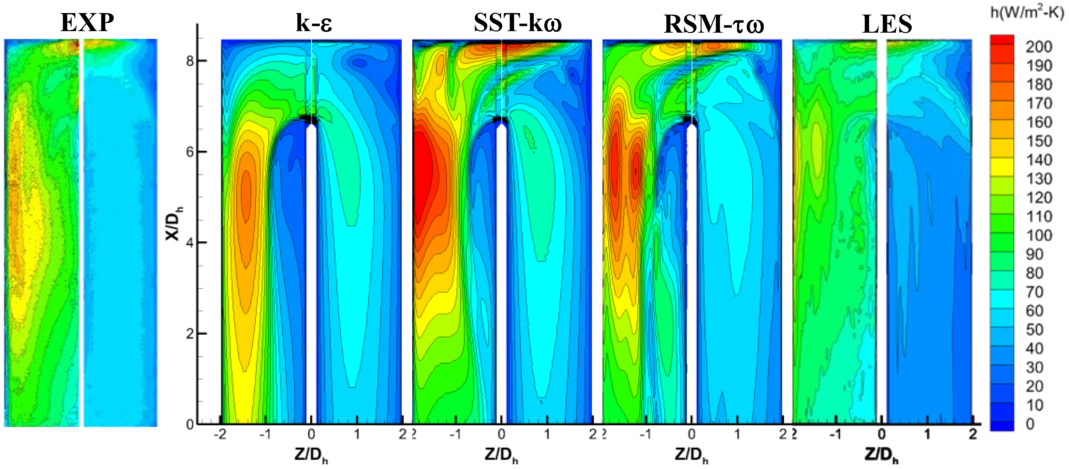
Figure 5.
Heat-transfer coefficient normalized by the maximum value h0 from RANS, LES, and EXP (represented by dots), where Z0 denotes the maximum Z of the domain.
Figure 5.
Heat-transfer coefficient normalized by the maximum value h0 from RANS, LES, and EXP (represented by dots), where Z0 denotes the maximum Z of the domain.

Figure 6.
Instantaneous velocity magnitude, V (m/s), in the “geometric” symmetry plane, and the frequency spectra measured at a probe located at ⊕ in the LES solution.
Figure 6.
Instantaneous velocity magnitude, V (m/s), in the “geometric” symmetry plane, and the frequency spectra measured at a probe located at ⊕ in the LES solution.

Figure 7.
Turbulent kinetic energy, TKE (), predicted by RANS and LES (for each trapezoid, left is the down-leg and right is the up-leg).
Figure 7.
Turbulent kinetic energy, TKE (), predicted by RANS and LES (for each trapezoid, left is the down-leg and right is the up-leg).

Figure 8.
Reynolds stresses predicted by RANS and LES.

Figure 9.
Pressure–strain rate at X/L1 = turn: RSM model using RSM and LES data and exact definition using LES data.
Figure 9.
Pressure–strain rate at X/L1 = turn: RSM model using RSM and LES data and exact definition using LES data.

Figure 10.
Comparison of turbulent diffusion calculated by RSM and LES data.

Figure 11.
Comparison of turbulent diffusion in the RSM model calculated by RSM data and in the exact definition calculated by LES data.
Figure 11.
Comparison of turbulent diffusion in the RSM model calculated by RSM data and in the exact definition calculated by LES data.

Figure 12.
Pressure diffusion vs. turbulent transport at X/L1 = 0.9.

Figure 13.
Pressure diffusion vs. turbulent transport at X/L1 = 0.8.

Figure 14.
Pressure diffusion vs. turbulent transport at X/L1 = 0.65.

Figure 15.
Pressure strain rate vs. pressure diffusion (exact definition) from LES at X/L1 = 0.8, turn, and 0.65.
Figure 15.
Pressure strain rate vs. pressure diffusion (exact definition) from LES at X/L1 = 0.8, turn, and 0.65.

Figure 16.
Evaluation of the eddy-diffusivity hypothesis of RANS: heat transport budget.

Figure 17.
Evaluation of RANS models on .

Figure 18.
Evaluation of RANS models on .

Figure 19.
Evaluation of RANS models on .

Figure 20.
Flow fields in corners of the up-leg near the inner wall (left) and the outer wall (right) on X/L1 = 0.5, colored by temperature (K): LES (top) vs. RSM (bottom).
Figure 20.
Flow fields in corners of the up-leg near the inner wall (left) and the outer wall (right) on X/L1 = 0.5, colored by temperature (K): LES (top) vs. RSM (bottom).

Figure 21.
Turbulent Prandtl number from LES (blue dotted lines denote the turn region).

Disclaimer/Publisher’s Note: The statements, opinions and data contained in all publications are solely those of the individual author(s) and contributor(s) and not of MDPI and/or the editor(s). MDPI and/or the editor(s) disclaim responsibility for any injury to people or property resulting from any ideas, methods, instructions or products referred to in the content. |
© 2024 by the authors. Licensee MDPI, Basel, Switzerland. This article is an open access article distributed under the terms and conditions of the Creative Commons Attribution (CC BY) license (https://creativecommons.org/licenses/by/4.0/).
Share and Cite
MDPI and ACS Style
Hu, K.S.; Shih, T.I.-P. Large-Eddy vs. Reynolds-Averaged Navier–Stokes Simulations of Flow and Heat Transfer in a U-Duct with Unsteady Flow Separation. Energies 2024, 17, 2414. https://doi.org/10.3390/en17102414
AMA Style
Hu KS, Shih TI-P. Large-Eddy vs. Reynolds-Averaged Navier–Stokes Simulations of Flow and Heat Transfer in a U-Duct with Unsteady Flow Separation. Energies. 2024; 17(10):2414. https://doi.org/10.3390/en17102414
Chicago/Turabian StyleHu, Kenny S., and Tom I-P. Shih. 2024. "Large-Eddy vs. Reynolds-Averaged Navier–Stokes Simulations of Flow and Heat Transfer in a U-Duct with Unsteady Flow Separation" Energies 17, no. 10: 2414. https://doi.org/10.3390/en17102414
Note that from the first issue of 2016, this journal uses article numbers instead of page numbers. See further details here.