
A Calculation Method for the Hyperspectral Imaging of Targets Utilizing a Ray-Tracing Algorithm


School of Physics, Xidian University, Xi’an 710071, China
*
Author to whom correspondence should be addressed.
Remote Sens. 2024, 16(10), 1779; https://doi.org/10.3390/rs16101779
Submission received: 28 March 2024
/
Revised: 3 May 2024
/
Accepted: 13 May 2024
/
Published: 17 May 2024
Abstract
:This paper proposes a hyperspectral imaging simulation method based on a ray-tracing algorithm. The algorithm combines calculations based on solar and atmospheric visible light radiation as well as the spectral bidirectional reflection distribution function (BRDF) of the target surface material and can create its own scenarios for simulation calculations on demand. Considering the presence of multiple scattering between the target and background, using the ray-tracing algorithm enables the precise computation of results involving multiple scattering. To validate the accuracy of the algorithm, we compared the simulated results with the theoretical values of the visible light scattering intensity from a Lambertian sphere. The relative error obtained was 0.8%. Subsequently, a complex scene of engineering vehicles and grass was established. The results of different observation angles and different coating materials were calculated and analyzed. In summary, the algorithm presented in this paper has the following advantages. Firstly, it is applicable to geometric models composed of any triangular mesh elements and accurately computes the effects of multiple scattering. Secondly, the algorithm combines the spectral BRDF information of materials and improves the efficiency of multiple scattering calculations using nonuniform sampling. The computed hyperspectral scattering data can be applied to simulate airborne or space-borne remote sensing data.

1. Introduction
Hyperspectral imaging technology, which gradually took shape in the 1970s, is a spectral technique that has revolutionized traditional discrete-point imaging methods. It integrates image information with spectral data, encompassing continuous spectral bands and a wide range of spectra. This enables a more comprehensive description of the scattering characteristics of targets. Consequently, research on hyperspectral imaging has become a hot topic in the study of target-scattering properties. Due to the distinct spectral characteristics of different targets, people can classify and identify the targets contained in images [1] and extract features of hyperspectral images and targets [2,3]. These research findings have wide-ranging applications in both military and civilian fields. Using satellite-borne hyperspectral cameras, hyperspectral images of the Earth’s surface can be obtained, enabling the identification [4] and classification of land types [5]. These cameras can also be used for scene classification, such as in the case of forests [6]. Hyperspectral images obtained from remote sensing satellites can also be used for maritime target detection [7], providing significant assistance in maritime rescue operations. In addition to remote sensing satellites, hyperspectral technology also has many applications in daily life. For example, in industry, it can be used to predict soil content in mines [8]. In agriculture, hyperspectral technology can be used for plant classification [9] and identification [10], crop yield prediction [11], and plant disease analysis [12]. In the medical field, hyperspectral technology has become an auxiliary tool for disease diagnosis [13].
Hyperspectral data are typically obtained through three main methods. The first method involves direct measurement using hyperspectral instruments. The second method involves acquiring data by expanding from multispectral data. The third method involves obtaining data through simulation and calculation. Direct measurement using hyperspectral instruments is the most effective method, as it allows for the acquisition of the most authentic and reliable data. For example, Summer Yarbrough et al. introduced the MightySat II.1 hyperspectral imager, which is the first spectrometer to operate in space [14]. D. Fort introduced the CONTOUR Remote Imager and Spectrograph (CRISP) instrument, which tracks the nuclei of comets, acquiring spectral information in the visible and infrared wavelengths. It is capable of conducting detailed measurements of gas and dust composition [15]. P. M. Teillet et al. introduced the use of the GER3700 spectrometer to collect surface reflectance spectral datasets at Cutbank Creek [16]. The drawback of using a hyperspectral instrument for measurement is the requirement of higher costs. For scenarios where directly measuring hyperspectral data is challenging, alternative methods can be utilized.
For scenarios where multispectral data are available, it is possible to extend the spectral range to obtain hyperspectral data. For example, methods such as non-negative matrix factorization can be used to generate hyperspectral images from multispectral data [17]. The fusion of hyperspectral and multispectral data based on bands can be employed to obtain hyperspectral data through spectral unmixing of multispectral data [18]. Alternatively, hyperspectral images can be obtained from low-spectral-resolution images using spectral library data [19]. To address the issue of low resolution in hyperspectral images, a method was proposed to fuse hyperspectral images with high-resolution images, enabling target identification [20]. However, these simulation methods require obtaining low-spectral-resolution data first and then using these data to simulate hyperspectral data, which may have certain limitations in practical applications.
In the absence of directly measured data, using physical models to simulate hyperspectral images of targets is an effective method. Hyperspectral imaging simulation involves considering results in both the spectral dimension and the spatial dimension. In terms of the spectral dimension, it is necessary to obtain spectral information of external radiation and the material spectral information of the target. There are many means to acquire spectral information of external radiation, and based on radiation transfer theory, some high-precision calculation methods have been proposed [21,22]. The computational speed of some of these methods can even be much higher than that of commonly used software [23]. During simulation, for the sake of computational convenience, mature software is typically employed for spectral calculations of radiation. The spectral information of target materials needs to be obtained through measured data, with the most common method being the utilization of remote sensing data to acquire the spectral reflectance of targets. For instance, Guo et al. utilized MODIS data to study the infrared reflection characteristics of aircraft [24]. V. García-Santos et al. conducted research on land surface temperature and emissivity based on MODIS data [25]. While using remote sensing data to obtain spectral reflectance is convenient, it may lack precision, especially in simulating near-field spectral characteristics. To address this issue, Cao et al. proposed a method to obtain the spectral bidirectional reflectance distribution function (BRDF) through measurements [26]. This method enables the acquisition of accurate material spectral BRDF data, facilitating high-precision calculations. The spectral BRDF in this study was also obtained using this method.
Once spectral dimension information is obtained, imaging simulation in the spatial dimension combined with spectral information can yield hyperspectral imaging data. There are typically two methods used for simulating imaging of targets. The first method involves using the 3D programming tool OpenGL for calculations [27]. For instance, Han computed space-based optical imaging of satellites [28], while Yu et al. conducted an infrared imaging simulation of ship targets [29], both utilizing the OpenGL tool for calculations. However, this method cannot compute results involving multiple scattering. The second method involves using ray-tracing algorithms for calculations, which can compute results including multiple scattering and has become the mainstream method for studying target scattering characteristics [30,31]. For example, Zhang et al. developed digital imaging simulation software using NVIDIA OptiX Ray Tracing Engine to simulate satellite targets [32]. However, during calculation, the satellite surface materials lacked spectral information, resulting in images without corresponding hyperspectral data. Additionally, there are other methods for simulating hyperspectral remote sensing images [33,34,35], but these methods rely on material libraries derived from remote sensing data, which may impose limitations in terms of accuracy and degrees of freedom during calculation. For example, Zhang et al. proposed a method for computing complex forest hyperspectral images, but the method lacks strong generality for other scenes [36]. Sun et al. proposed a method for simulating hyperspectral dynamic scenes, but it did not consider multiple scattering and the spectral BRDF of the material [37].
In summary, when acquiring hyperspectral data, directly measured data are the most accurate but often come with high costs. Spectral expansion methods require a foundation of multispectral data and may resort to simulation if spectral data are unavailable. However, existing simulation methods often lack in both material spectral data and multiple scattering calculations. To address these shortcomings and achieve more universal and accurate hyperspectral simulation data, this paper proposes a hyperspectral imaging simulation algorithm based on spectral BRDF data. This algorithm enables precise hyperspectral simulation calculations for targets. Compared to using remote sensing inversion methods for the spectral BRDF, this approach allows for more accurate simulation of target spectral properties. The simulation utilizes ray-tracing algorithms, encompassing results from multiple scattering simulations. This article first introduces the algorithm’s process and computational principles, then constructs the geometric scene of the target and conducts simulation calculations, and finally analyzes the simulation results.
2. Methodology
Figure 1 shows the hyperspectral image calculation flow described in this paper.
In the algorithm described in this paper, the geometric model of the target is first established according to the requirements. After obtaining the geometric model of the target, we set up materials for the different parts of the target. The spectral BRDF parameters of the material can be obtained through actual measurements and calibrations. Radiation information on the sun and atmosphere can be obtained according to the radiation transfer theory, but this aspect is not the focus of this paper; this paper uses Modtran to calculate the radiation information. After obtaining radiation information on the environment, the hyperspectral scattering results of the target are calculated using a ray-tracing algorithm. By changing the calculation conditions, different results can be obtained, and these results can be analyzed.
2.1. Computation of Scattering Characteristics Utilizing the Ray-Tracing Method
Figure 2 illustrates the simulation flow of target-scattering characteristics using a ray-tracing algorithm.
In the simulation, the imaging resolution is established based on the accuracy requirements. Subsequently, the ray projection scale is determined in accordance with the resolution, and the ray is initialized upon completion. During the calculation process, the backward tracking method is utilized, requiring an assessment of whether the ray can intersect with the model based on the observation direction. If there is no intersection, this implies that the current ray does not observe anything. The subsequent procedure involves emitting rays from the intersection towards the light source and ascertaining the presence of any obstructing objects between the intersection and the light source. Light can only reach the intersection if there are no obstructions. Ultimately, the imaging outcomes can be derived through the computation of ray scattering intensity, which is based on the spectral BRDF data of the material surface and the incident light’s irradiance. In the context of intersection judgment, it is assumed that the coordinates of the starting point of the ray are denoted as and the direction of ray projection is denoted as . Utilizing three vectors, , , and , to denote the positions of the three vertices of the triangular surface, any point on the plane where the triangle is situated can be expressed as . The equation is established to determine the position of as the intersection point between the ray and the plane of the triangle. Thus, we can know
By solving Equation (1), the values of u, v, and t can be obtained. When the intersection points are located within a triangle, u, v, and t must satisfy the following conditions:
Figure 3 briefly illustrates the occlusion culling process in the ray tracing algorithm. In accordance with the aforementioned method, it is feasible to determine whether the ray intersects the triangle. Given the generally more complex nature of the target model, a series of intersection points may be obtained following the intersection judgment. In this instance, the more distant points will be obstructed by the nearer points, necessitating the identification of the nearest intersection. The occlusion of the ray between the intersection point and the light source is also determined using the aforementioned method. If the ray projected from the intersection point to the light source does not intersect with any triangle, the light path represented by this ray is considered feasible, and the scattering intensity of this ray can be computed.
Assuming light enters from direction and is received from direction , it can be understood that the scattered radiance of a single ray is the superposition of the single-scattering result and the multiple-scattering result. The scattered radiance of single scattering can be expressed as
Here, represents the direct irradiance in the direction of the light source, represents the irradiance on the normal direction of the intersecting surface element, and represents the BRDF specified for the incident and scattering directions. When calculating multiple scattering, it is necessary to track the energy distribution characteristics of scattering on the material surface at the single scattering points. The Monte Carlo method is employed to sample the rays for multiple scattering during the computation. The radiance of multiple scattering can be expressed as
where represents the differential solid angle. The total scattered radiance on a single surface element can be expressed as
Assuming that represents the BRDF of the material, the formula for calculating the ray scattering radiance is
In Equation (6), represents the spectral irradiance of incident light, while , , , and denote the incident zenith angle, receiving zenith angle, incident azimuth angle, and receiving azimuth angle, respectively, within the plane coordinate system. By integrating it with visible light, the radiance of each ray within the visible light spectrum can be determined.
2.2. Sampling and Optimizing Multiple Scatterings
In our investigation of the computational aspects of multiple scatterings, we utilized the ray-splitting method and conducted sampling in the hemisphere space to simulate the spatial distribution of scattered energy. Augmenting the sample size can improve computational precision, but it also leads to a substantial increase in the computation time as a result of the corresponding rise in workload. Therefore, it is essential to find a balance between the quantity of samples and computational accuracy, while considering the trade-off between precision and computational efficiency. The most effective approach entails reducing the number of ray-splitting samples without sacrificing computational accuracy; this is achieved through the optimization of the sampling method in combination with the spatial distribution of scattered energy. The core concept of ray splitting involves the use of sampling for integral calculations. Due to the uneven distribution of scattered energy in the hemisphere space, areas with lower scattered energy make a smaller contribution to the overall result, whereas regions with higher scattered energy exert a more significant influence. Hence, it is essential to augment the sampling density in these highly scattered energy regions by employing importance sampling methods to improve sampling efficiency while maintaining accuracy. The specific methodology was outlined in a previous publication; however, a concise summary will be presented here [38].
In the case of a standard rough surface, the energy scattered by incoming light will be dispersed within a specific solid angle around the direction of specular reflection. The range of solid angles varies depending on the roughness of the material. Glossier materials are characterized by a smaller solid angle, whereas rougher materials exhibit a larger solid angle. The solid angle ranges from 0 to , encompassing the majority of material types found in typical surfaces. When computing the scattering from a typical rough surface, the range of scattered light can be estimated by employing a conical spherical cap with the specular reflection direction as its axis.
In order to sample the multiple scattered light in the conical spherical crown space, it is necessary to first determine the solid angle of the conical spherical crown. The solid angle size can be determined based on the BRDF characteristics of the material [39,40]. The sampling method is shown in Figure 4. If the solid angle of the conical spherical crown is excessive, this will result in minimal scattering in specific spatial regions. This phenomenon can have a significant impact on the accuracy of approximations, necessitating a greater number of samples to achieve the same level of precision and consequently influencing the computational efficiency. Conversely, a conical spherical crown with a small solid angle may exclude some scattering from the calculations, leading to computed values that are relatively smaller than the actual values. Upon determining the apex angle of the solid angle cone as , the calculation of the solid angle occupied by the conical spherical crown, with the corresponding angular size, is provided by
2.3. Measurement and Modeling of BRDF
Prior to acquiring the material’s BRDF, it is essential to measure the material sample using a suitable instrument. The samples are manipulated at different angles with the use of a motor, enabling the measuring of various incident and reflection angles. The light emitted from the light source is collimated and directed towards the material samples. Subsequently, the radiometer is utilized to capture the reflected data. The use of a halogen tungsten lamp as the light source enables the emission of a consistent and uninterrupted spectrum. The measuring device can be used to measure the spectral radiance of the sample at various angles. A comparison of the spectral radiance of the sample with that of a standard reference board enables the determination of the sample’s spectral BRDF. For instance, if the angle of light incidence on the sample is , the calibration formula can be represented as Equation (8).
In the given equation, represents the spectral radiation brightness of incident light, with wavelength , that is directed onto the sample to be measured along the direction and received along the direction; denotes the spectral radiation brightness received along the direction under the same conditions, where incident light with the same wavelength is directed onto the standard plate along the direction. represents the BRDF of the target sample at the incident wavelength . When describing BRDF, a five-parameter model [41] is utilized, and the expression of the five-parameter model is as follows:
where , , b, a, and indicate the parameters to be determined.
3. Analysis and Results
3.1. Spectral BRDF of Some Materials
In order to obtain material BRDF data that can be used for calculation, we made samples of four common colors—black, white, gray, and gray-green—for measurement. When making the sample, a steel disc with a thickness of about 1.5 mm was selected and painted. The surface of the sample was smooth and flat after repeated spraying. When measuring the spectral BRDF of a sample, a comparative measurement method was employed. By using the spectral radiance of the standard whiteboard as a reference, the BRDF of the sample could be obtained. The measurement formula is
where represents the BRDF of the target sample at wavelength . represents the spectral radiance of the light incident along direction onto the sample and scattered along direction . represents the spectral radiance of the light incident along direction onto the standard whiteboard and scattered along direction . represents the reflectance of the standard whiteboard at wavelength . , , , and , respectively, represent the incidence zenith angle, scattering zenith angle, incidence azimuth angle, and scattering azimuth angle.
During measurements, a halogen lamp served as the light source, emitting a stable continuous spectrum. The sample was fixed on a turntable, and a computer controlled the motor to rotate it at different angles while recording the spectral radiance data scattered from the sample received by the radiometer. Through these measurements, the spectral BRDF parameters of the sample could be obtained.
Based on the principles described in the previous section, we performed spectral BRDF measurements on four different color samples and performed five-parameter modeling. Among these, the spectral BRDF modeling results of the white sample are shown in Table 1.
The results of the remaining colors are presented in the same way as the white sample and are represented by five parameters. Using the five-parameter results obtained from the measurement, it is possible to compute the spectral BRDF at various incidence angles, scattering angles, and wavelengths.
Figure 5 depicts the spectral BRDF results of the four materials at various observation angles, with the light incident set at a 30-degree angle. The spectral BRDF calculation results demonstrate distinct scattering characteristics for different materials. In comparison to the black material, the white material exhibits higher reflectivity. Both materials display distinct reflection peaks at the mirror position. The impact is heightened when the secondary-scattering sampling algorithm, as discussed in Section 2, is employed for such materials. The spatial reflection of materials in shades of gray and gray-green is more uniform, with no prominent reflection peak. The spectral BRDF findings for the four materials indicate variations in the scattering properties across both spatial and spectral dimensions.
3.2. Spectral Radiation of Sunlight and Atmosphere
The electromagnetic waves and particle flow emitted by the sun into space are referred to as solar radiation. This radiation is equivalent to the capacity of 6000 K blackbody radiation and serves as the most important energy source for Earth’s surface activities. Solar radiation energy exhibits significant variation across different wavelengths, with a notable disparity in energy distribution within the spectral range. Approximately 99% of the energy is concentrated in the spectral range of 0.15–4 m, with the visible band (0.4 m to 0.76 m) accounting for approximately 50% of this energy. The remaining 50% is distributed across the infrared and ultraviolet bands.
Solar irradiance denotes the amount of solar radiation reaching the Earth’s surface following absorption, scattering, reflection, and other attenuating effects of the atmosphere. Attenuation primarily encompasses the absorption and scattering of atmospheric molecules and dust, as well as the scattering of clouds and dust particles within the atmosphere. Solar radiation reaching the Earth’s surface is influenced by various factors, including latitude, longitude, altitude, and atmospheric conditions.
In this paper, MODTRAN was utilized for radiation transfer calculations. The simulation was set for 12:00 p.m. on 1 May 2023, Beijing Time. Suppose it is a sunny day in Xi’an, with a local latitude of 34°1540N and a longitude of 108°5632E. The calculated results of solar irradiance are depicted in Figure 6.
Upon reaching the Earth’s atmospheric system, a portion of solar radiation is reflected and scattered back into space, while the remainder penetrates the atmospheric system. A portion of the solar radiation that reaches the Earth’s surface is directly projected in the form of parallel light, and this portion is referred to as direct solar radiation. The remaining portion of the light reaches the Earth’s surface as a result of the absorption, scattering, and reflection by atmospheric molecules, particles, and water vapor, constituting sky background radiation. The computed outcomes of atmospheric radiation are depicted in Figure 7.
The algorithm does not account for atmospheric radiative transfer effects caused by weather conditions such as rain, snow, or fog. Therefore, the algorithm proposed in this paper is currently only suitable for simulating hyperspectral imaging of targets under ideal lighting conditions.
3.3. Algorithm Accuracy Verification
To validate the precision of our algorithm, we chose a spherical model with theoretical solutions for simulation, and we subsequently compared the simulation results with the theoretical outcomes. The theoretical scattering intensity of a sphere in the visible band can be determined under the assumption that the sphere’s surface is a Lambertian material.
The angle of calculation involves a backward observation, as depicted in Figure 8. Equation (11) expresses the scattering radiance of the observable portion of the target’s solar irradiance.
In Equation (11), represents the incident zenith angle of the target skin material sample’s BRDF. The symbols , , and represent the incident zenith angle, detection zenith angle, and relative azimuth angle, respectively, within the plane coordinate system. represents the solar irradiance at the specified altitude of the target.
Equation (12) depicts the scattering of sky background radiation by the visible part of the target.
In Equation (12), represents the surface element BRDF, is the sky background radiance at the height of the incident target in the direction , and correspond to the incident celestial angle and azimuth angle in the target coordinate system, and signifies the unit solid angle.
By integrating the upper hemisphere space, one can obtain the scattering brightness of surface elements against the background radiance of the sky.
Assuming the incident light source is sunlight, the spectral scattering brightness of a single surface element at wavelength is represented by Equation (14).
denotes the BRDF at the specific wavelength , while signifies the spectral irradiance of sunlight at the same wavelength . The scattering intensity can be represented by Equation (15).
The variable “S” in the equation represents the area of the element. Equation (16) displays the spectral scattering intensity of the entire target at wavelength .
In the equation, “l” denotes the number of facet elements, while “N” represents the total number of facet elements. The symbols , , , and denote the incident zenith angle, incident azimuth angle, scattering zenith angle, and scattering azimuth angle, respectively, in the plane coordinate system. The symbol denotes the spectral irradiance of sunlight at a specific wavelength . For a Lambert sphere, the theoretical spectral scattering intensity at a given wavelength can be determined using Equation (16).
The analytical solution for the scattering intensity of the Lambert sphere, when light of wavelength to is incident, can be obtained from Equation (17), as shown in Equation (18).
A Lambertian sphere with a surface spectral reflectance of was chosen for verification. The ball had a diameter of 1 m, and the incident light source consisted of visible light with a wavelength ranging from 400 nm to 760 nm. The irradiance of the light source was calculated using the MODTRAN 5.2 software, assuming clear weather conditions with good visibility. The theoretical value of the scattering intensity of the sphere, as derived from Equation (18), was 87.8455 . The ray-tracking algorithm was used to simulate the scattering intensity of a Lambert sphere under identical conditions, resulting in a scattering intensity of 87.1067 . The relative error between the simulation results and analytical solutions was 0.8%. The findings indicate that the simulation algorithm demonstrates a high level of accuracy, thereby establishing a solid foundation for subsequent research endeavors.
4. Discussion
4.1. Geometric Model of the Target
To investigate the spectral characteristics of visible light in the target, a setup was created with an engineering vehicle parked on grass. The grass area measured 40 by 40 m, and the surface of the engineering vehicle was coated with gray-green paint, as described in Section 3. As depicted in Figure 9, the geometric representation of the grassland consists of a gridded plane with varying elevations.
The engineering vehicle was placed in a central position on the grass, as shown in Figure 10.
The spectral scattering properties of grassland are characterized by a three-parameter BRDF model of the kernel drive function [42], the formula of which is presented in Equation (19).
In Equation (19), represents the zenith angle of the incident sunlight, represents the observation zenith angle of the satellite, and signifies the relative azimuth angle between the incident sunlight direction and the observation direction of the satellite. represents the Ross-thick core, while represents the Li-Transit core. The variables , , and denote the weights assigned to each core, and their respective values can be derived from MODIS satellite data. The MODIS satellite data include four channels that capture visible light:
- band1: 620–670 nm;
- band2: 841–846 nm;
- band3: 459–479 nm;
- band4: 545–565 nm.
Table 2 displays the parameter selection for the four bands of grassland BRDF.
4.2. Hyperspectral Imaging of the Target
As depicted in Figure 11, the x axis represents the front direction of the engineering vehicle, the y axis represents the left side of the engineering vehicle, and the z axis represents the right side of the engineering vehicle.
4.2.1. The Outcomes under Various Observation Angles
Based on the given longitude, latitude, and time, it can be determined that the solar zenith angle was 21.6 and the solar azimuth angle was 149. The visible light scattering image of the target when the observation zenith angle is 0 and the observation azimuth angle is 90 is depicted in Figure 12.
Figure 12 depicts the scattering radiance image of the target in the visible band, providing a more accurate representation of the distribution of light and shade. To acquire a more comprehensive understanding of the scattering characteristics of the target, it is necessary to calculate them from various observation angles. Figure 13 depicts the calculated results for various observation zenith angles while maintaining a consistent observation azimuth.
The calculation results indicate that at different solar zenith angles, the scattered radiance of the grassland remains relatively constant. This is because the BRDF (bidirectional reflectance distribution function) characteristics of the grassland are similar to those of Lambertian materials, with relatively uniform scattering distributions in all directions. When observed from different angles, the inclined surfaces of the engineering vehicle appear brighter, manifesting as a bright band in the image, with the radiance on the inclined surfaces exceeding that of the vehicle roof by over 50%. This is attributed to the smaller solar zenith angle when observing the inclined surfaces. With changes in the solar zenith angle, at 30, bright spots resulting from specular reflection can be observed in certain areas, while they are less prominent at other angles. As the solar zenith angle increases from 30 to 60, the observed solar zenith angle on the side of the vehicle gradually decreases, leading to an increase in radiance. When the solar zenith angle changes to 60, the radiance on the side of the vehicle increases by approximately 33%. Conversely, the radiance on the vehicle roof decreases by about 25%.
Figure 14 and Figure 15 depict visible light scattering images at a solar zenith angle of 45 under different azimuth angles. The influence of sunlight and viewing angles is clearly visible in the visible light images. When the azimuth angle is 90, a significant bright band is observed due to the more direct sunlight exposure. At an azimuth angle of 270, most of the observed areas are not directly exposed to sunlight, resulting in increased shadow areas. Additionally, the positions of specular reflections vary with the azimuthal observation angle. When the azimuth angle is 0, the brightest position is located at the front of the vehicle. At an azimuth angle of 90, the brightest position is on the inclined surface of the vehicle roof. At an azimuth angle of 180, the brightest position is at the rear of the vehicle and on the raised portion of the roof. At an azimuth angle of 270, the brightest position is on the vehicle roof. When the azimuth angle is 0, the radiance at the brightest position is approximately 25% higher compared to when the azimuth angle is 90, and nearly twice as high compared to when the azimuth angle is 270.
In Figure 16, we compare the visible light scattering images of engineering vehicles with different materials under the same observation conditions. In Figure 16a, the surface of the engineering vehicle is made of gray-green material, while in Figure 16b, the surface is made of white material. The spectral BRDF of these materials can be found in Section 3. When the surface of the engineering vehicle is made of gray-green material, the radiance at most positions is similar to that of the grassland. However, when the surface of the engineering vehicle is made of white material, the scattered radiance on the vehicle surface is significantly higher than that of the grass. The radiance of the white material is nearly twice as high as that of the gray-green material. These calculation results also align with common sense.
4.2.2. The Outcomes for Different Paint Types
The aforementioned findings depict images of the visible light spectrum in its entirety. However, hyperspectral images have the capacity to encompass additional information, including scattering imaging at various wavelengths. The hyperspectral image was chosen with an observation zenith angle of 0 degrees and an observation azimuth angle of 0 degrees. Subsequently, the hyperspectral data were extracted for analysis.
As illustrated in Figure 17, a specific location atop the engineering vehicle was chosen, and the spectral scattering curves of white spray paint and gray-green spray paint were individually extracted for comparative analysis.
As shown in Figure 18, the scattering spectral curves reveal noticeable differences between the two materials. This discrepancy can be attributed to the distinct spectral scattering characteristics exhibited by various materials. When combined with spectral BRDF, it becomes evident that the spectral scattering curves of white paint and gray-green paint align with the pattern of spectral BRDF variations across different wavelengths. This also confirms the validity of the calculation results.
To gain a more intuitive understanding of the scattering characteristics of the target scene across various wavelengths, we can extract scattering images corresponding to different wavelengths from the hyperspectral image for further analysis.
As shown in Figure 19, under consistent lighting conditions, coatings of different colors exhibit significant variations in scattering patterns at different wavelengths. In the case of white paint, the engineering vehicle’s scattered radiance at a wavelength of 430 nm is approximately double that of the surrounding grass background. However, as the wavelength shifts to 720 nm, the brightness of the engineering vehicle becomes very similar to the background. Conversely, for gray-green paint, the engineering vehicle’s scattered radiance at 430 nm is approximately 37% lower than that of the surrounding grass background. At 720 nm, the engineering vehicle’s scattering brightness is also closer to the background. This observed trend aligns logically with the spectral scattering curves depicted in Figure 1. Hence, it can be inferred that the simulation results of hyperspectral scattering are advantageous for the analysis of target characteristics.
4.2.3. The Outcomes of Sunlight Scattering, Atmospheric Scattering, and Multiple Scatterings
Figure 20 presents the results of multiple-scattering calculations for the target under the influence of solar radiation, atmospheric radiation, and the interaction between the target and the background. The observation zenith angle is 45 degrees, and the azimuth angle is 90 degrees. The results indicate that due to the significant direct irradiance from the sun, the target exhibits the highest scattered radiance in response to solar radiation. However, because of the limited area directly illuminated by sunlight, there are considerable shadow regions in the visible light image.
Conversely, as atmospheric radiation is omnipresent in the entire space, the shadowing effect in the scattered atmospheric radiation image is minimal. Multiple scatterings between the target and background primarily occur in the dihedral angle structure, and these are predominantly concentrated on the vehicle’s side. In numerical terms, each of these three components contributes significantly, and their proportional representation in the simulation calculations cannot be overlooked.
5. Conclusions
This paper introduces a hyperspectral simulation algorithm that combines spectral BRDF with ray tracing. By utilizing the spectral BRDF of materials in the calculations, the results are more accurate. The validation of the method was conducted by comparing theoretical values with simulation results. A spherical model with a diameter of 1 m was chosen, assuming the surface to be a Lambertian material with a reflectance of 1. Spectral scattering intensities were calculated using both the algorithm proposed in this paper and theoretical methods. The relative error between the two methods was found to be 0.8%, confirming the accuracy of the proposed algorithm. In subsequent discussions, we established a practical scenario involving an engineering vehicle positioned on grass. Simulations were performed from various angles, generating a comprehensive dataset. A detailed analysis of the computed results was conducted, with a comparison and discussion of the data observed at different angles of observation. The findings suggest that our algorithm demonstrates exceptional simulation performance.
Hyperspectral technology is currently widely applied in various fields. The algorithm proposed in this paper can provide simulated data for training models in hyperspectral identification research and also assist in the study of material and target characteristics. The algorithm is applicable to any scene that can be geometrically modeled and to isotropic surface materials. By utilizing the spectral BRDF, this algorithm is suitable not only for far-field hyperspectral scattering calculations but also for near-field calculations. In future research, we aim to expand the simulated bands to include calculations for additional spectra such as infrared. Currently, the algorithm does not account for atmospheric radiative transmission effects caused by weather conditions such as clouds, fog, rain, or snow. Calculations under nonideal lighting conditions will also be a focus of future research.
Author Contributions
Conceptualization, Y.C. (Yisen Cao) and Y.C. (Yunhua Cao); methodology, Y.C. (Yunhua Cao) and Z.W.; data curation, Y.C. (Yisen Cao); validation, Y.C. (Yisen Cao); writing—original draft, Y.C. (Yisen Cao) and K.Y.; writing—review and editing, Y.C. (Yunhua Cao) and K.Y. All authors have read and agreed to the published version of the manuscript.
Funding
This research is supported by the 111 Project (Grant No. B17035).
Data Availability Statement
This study utilized publicly available data from the Moderate Resolution Imaging Spectroradiometer (MODIS) provided by NASA. These datasets can be freely accessed through NASA’s Earthdata website at [https://ladsweb.modaps.eosdis.nasa.gov (accessed on 27 March 2024)].
Acknowledgments
The authors express gratitude to the reviewers for their careful evaluation. We express our gratitude for the valuable comments and suggestions provided.
Conflicts of Interest
The authors declare no conflicts of interest.
Abbreviations
The following abbreviations are used in this manuscript:
| BRDF | Bidirectional reflection distribution function |
References
- Zhang, L.; Lu, H.; Zhang, H.; Zhao, Y.; Xu, H.; Wang, J. Hyper-Spectral Characteristics in Support of Object Classification and Verification. IEEE Access 2019, 7, 119420–119429. [Google Scholar] [CrossRef]
- Li, L.; Gao, J.; Ge, H.; Zhang, Y.; Zhang, H. An effective feature extraction method via spectral-spatial filter discrimination analysis for hyperspectral image. Multimed. Tools Appl. 2022, 81, 40871–40904. [Google Scholar] [CrossRef]
- Wang, J.; Nian, F.; Chen, Z.; Liu, G. A calculation method for Spatially Varying Bidirectional Reflection Factor of target based on hyper-spectral image sequence. Opt. Commun. 2021, 482, 126598. [Google Scholar] [CrossRef]
- Stević, D.; Hut, I.; Dojčinović, N.; Joković, J. Automated identification of land cover type using multispectral satellite images. Energy Build. 2016, 115, 131–137. [Google Scholar] [CrossRef]
- Suresh, S.; Lal, S. A metaheuristic framework based automated Spatial-Spectral graph for land cover classification from multispectral and hyperspectral satellite images. Infrared Phys. Technol. 2020, 105, 103172. [Google Scholar] [CrossRef]
- Awad, M.M.; Lauteri, M. Self-Organizing Deep Learning (SO-UNet)—A Novel Framework to Classify Urban and Peri-Urban Forests. Sustainability 2021, 13, 5548. [Google Scholar] [CrossRef]
- Park, J.J.; Park, K.A.; Kim, T.S.; Oh, S.; Lee, M. Aerial hyperspectral remote sensing detection for maritime search and surveillance of floating small objects. Adv. Space Res. 2023, 72, 2118–2136. [Google Scholar] [CrossRef]
- Pudełko, A.; Chodak, M.; Roemer, J.; Uhl, T. Application of FT-NIR spectroscopy and NIR hyperspectral imaging to predict nitrogen and organic carbon contents in mine soils. Measurement 2020, 164, 108117. [Google Scholar] [CrossRef]
- Bhujade, V.G.; Sambhe, V. Role of digital, hyper spectral, and SAR images in detection of plant disease with deep learning network. Multimed. Tools Appl. 2022, 81, 33645–33670. [Google Scholar] [CrossRef]
- Salve, P.; Yannawar, P.; Sardesai, M. Multimodal plant recognition through hybrid feature fusion technique using imaging and non-imaging hyper-spectral data. J. King Saud Univ.-Comput. Inf. Sci. 2022, 34, 1361–1369. [Google Scholar] [CrossRef]
- Sathiyamoorthi, V.; Harshavardhanan, P.; Azath, H.; Senbagavalli, M.; Viswa Bharathy, A.M.; Chokkalingam, B.S. An effective model for predicting agricultural crop yield on remote sensing hyper-spectral images using adaptive logistic regression classifier. Concurr. Comput. Pract. Exp. 2022, 34, e7242. [Google Scholar] [CrossRef]
- Park, K.; ki Hong, Y.; hwan Kim, G.; Lee, J. Classification of apple leaf conditions in hyper-spectral images for diagnosis of Marssonina blotch using mRMR and deep neural network. Comput. Electron. Agric. 2018, 148, 179–187. [Google Scholar] [CrossRef]
- Tian, C.; Su, W.; Huang, S.; Shao, B.; Li, X.; Zhang, Y.; Wang, B.; Yu, X.; Li, W. Identification of gastric cancer types based on hyperspectral imaging technology. J. Biophotonics 2023, 17, e202300276. [Google Scholar] [CrossRef] [PubMed]
- Yarbrough, S.; Caudill, T.R.; Kouba, E.T.; Osweiler, V.; Arnold, J.; Quarles, R.; Russell, J.; Otten III, L.J.; Al Jones, B.; Edwards, A.; et al. MightySat II. 1 hyperspectral imager: Summary of on-orbit performance. In Imaging Spectrometry VII; SPIE: Philadelphia, PA, USA, 2002; Volume 4480, pp. 186–197. [Google Scholar]
- Fort, D.; Warren, J.; Strohbehn, K.; Murchie, S.; Heyler, G.; Peacock, K.; Boldt, J.; Darlington, E.; Hayes, J.; Henshaw, R.; et al. The CONTOUR remote imager and spectrograph. Acta Astronaut. 2003, 52, 427–431. [Google Scholar] [CrossRef]
- Teillet, P.; Fedosejevs, G.; Gauthier, R. Operational radiometric calibration of broadscale satellite sensors using hyperspectral airborne remote sensing of prairie rangeland: First trials. Metrologia 1998, 35, 639. [Google Scholar] [CrossRef]
- Huang, Z.; Chen, Q.; Chen, Q.; Liu, X.; He, H. A Novel Hyperspectral Image Simulation Method Based on Nonnegative Matrix Factorization. Remote Sens. 2019, 11, 2416. [Google Scholar] [CrossRef]
- Li, X.; Yuan, Y.; Wang, Q. Hyperspectral and multispectral image fusion based on band simulation. IEEE Geosci. Remote Sens. Lett. 2019, 17, 479–483. [Google Scholar] [CrossRef]
- Chen, F.; Niu, Z.; Sun, G.; Wang, C.; Teng, J. Using low-spectral-resolution images to acquire simulated hyperspectral images. Int. J. Remote Sens. 2008, 29, 2963–2980. [Google Scholar] [CrossRef]
- Chen, H.; Du, X.; Liu, Z.; Cheng, X.; Zhou, Y.; Zhou, B. Target recognition algorithm for fused hyperspectral image by using combined spectra. Spectrosc. Lett. 2015, 48, 251–258. [Google Scholar] [CrossRef]
- Moncet, J.L.; Uymin, G.; Lipton, A.E.; Snell, H.E. Infrared radiance modeling by optimal spectral sampling. J. Atmos. Sci. 2008, 65, 3917–3934. [Google Scholar] [CrossRef]
- Su, M.; Liu, C.; Di, D.; Le, T.; Sun, Y.; Li, J.; Lu, F.; Zhang, P.; Sohn, B.J. A Multi-Domain Compression Radiative Transfer Model for the Fengyun-4 Geosynchronous Interferometric Infrared Sounder (GIIRS). Adv. Atmos. Sci. 2023, 40, 1844–1858. [Google Scholar] [CrossRef]
- Liu, X.; Yang, Q.; Li, H.; Jin, Z.; Wu, W.; Kizer, S.; Zhou, D.K.; Yang, P. Development of a fast and accurate PCRTM radiative transfer model in the solar spectral region. Appl. Opt. 2016, 55, 8236–8247. [Google Scholar] [CrossRef] [PubMed]
- Guo, X.; Wu, Z.; Wu, J.; Cao, Y. Study of infrared reflection characteristics of aerial target using MODIS data on GPU. J. Real-Time Image Process. 2018, 15, 643–655. [Google Scholar] [CrossRef]
- García-Santos, V.; Coll, C.; Valor, E.; Niclòs, R.; Caselles, V. Analyzing the anisotropy of thermal infrared emissivity over arid regions using a new MODIS land surface temperature and emissivity product (MOD21). Remote Sens. Environ. 2015, 169, 212–221. [Google Scholar] [CrossRef]
- Cao, Y.; Wu, Z.; Zhang, H.; Wei, Q.; Wang, S. Experimental Measurement and Statistical Modeling of Spectral Bidirectional Reflectance Distribution Function of Rough Target Samples. Ph.D. Thesis, Shanghai University of Electric Power, Shanghai, China, 2008. [Google Scholar]
- Chen, B.; Cheng, H.H. Interpretive OpenGL for computer graphics. Comput. Graph. 2005, 29, 331–339. [Google Scholar] [CrossRef]
- Han, Y.; Lin, L.; Sun, H.; Jiang, J.; He, X. Modeling the space-based optical imaging of complex space target based on the pixel method. Optik 2015, 126, 1474–1478. [Google Scholar] [CrossRef]
- Yu, C.; Zhang, H.; Zheng, G. Research on infrared imaging simulation technology of ocean scene. In AOPC 2021: Optical Sensing and Imaging Technology; SPIE: Philadelphia, PA, USA, 2021; Volume 12065, pp. 255–259. [Google Scholar]
- Han, Y.; Sun, H.; Li, Y.; Guo, H. Fast calculation method of complex space targets’ optical cross section. Appl. Opt. 2013, 52, 4013–4019. [Google Scholar] [CrossRef] [PubMed]
- Han, Y.; Sun, H.; Guo, H. Analysis of influential factors on a space target’s laser radar cross-section. Opt. Laser Technol. 2014, 56, 151–157. [Google Scholar] [CrossRef]
- Zhang, Y.; Lv, L.; Yang, C.; Gu, Y. Research on digital imaging simulation method of space target navigation camera. In Proceedings of the 2021 IEEE 16th Conference on Industrial Electronics and Applications (ICIEA), Chengdu, China, 1–4 August 2021; IEEE: New York, NY, USA, 2021; pp. 1643–1648. [Google Scholar]
- Arnold, P.S.; Brown, S.D.; Schott, J.R. Hyperspectral simulation of chemical weapon dispersal patterns using DIRSIG. In Targets and Backgrounds VI: Characterization, Visualization, and the Detection Process; SPIE: Philadelphia, PA, USA, 2000; Volume 4029, pp. 288–299. [Google Scholar]
- Börner, A.; Wiest, L.; Keller, P.; Reulke, R.; Richter, R.; Schaepman, M.; Schläpfer, D. SENSOR: A tool for the simulation of hyperspectral remote sensing systems. ISPRS J. Photogramm. Remote Sens. 2001, 55, 299–312. [Google Scholar] [CrossRef]
- Goodenough, A.A.; Brown, S.D. DIRSIG5: Next-generation remote sensing data and image simulation framework. IEEE J. Sel. Top. Appl. Earth Obs. Remote Sens. 2017, 10, 4818–4833. [Google Scholar] [CrossRef]
- Zhang, J.; Zhang, X.; Zou, B.; Chen, D. On hyperspectral image simulation of a complex woodland area. IEEE Trans. Geosci. Remote Sens. 2010, 48, 3889–3902. [Google Scholar] [CrossRef]
- Sun, D.; Gao, J.; Sun, K.; Hu, Y.; Li, Y.; Xie, J.; Zhang, L. Research on hyperspectral dynamic scene and image sequence simulation. In Hyperspectral Remote Sensing Applications and Environmental Monitoring and Safety Testing Technology; SPIE: Philadelphia, PA, USA, 2016; Volume 10156, pp. 323–330. [Google Scholar]
- Cao, Y.; Cao, Y.; Li, W.; Bai, L.; Wu, Z.; Wang, Z. Optimization of ray tracing algorithm for laser radar cross section calculation based on material bidirectional reflection distribution function. Opt. Commun. 2021, 500, 127207. [Google Scholar] [CrossRef]
- Culpepper, M.A. Empirical bidirectional reflectivity model. In Targets and Backgrounds: Characterization and Representation; SPIE: Philadelphia, PA, USA, 1995; Volume 2469, pp. 208–219. [Google Scholar]
- Wu, Z. Experimental study on bidirectional reflectance distribution function of laser scattering from various rough surfaces. Acta Opt. Sin. 1996, 16, 262–268. [Google Scholar]
- Zhang, H.; Wu, Z.; Cao, Y.; Zhang, G. Measurement and statistical modeling of BRDF of various samples. Opt. Appl. 2010, 40, 197–208. [Google Scholar]
- Hua, Y.; Xiao, L.I.; Feng, G. An Algorithm for the Retrieval of Albedo from Space Using New GO Kernel-Driven BRDF Model. J. Remote Sens. 2002, 6, 246–251. [Google Scholar]
Figure 1.
Calculation flow of hyperspectral imaging.
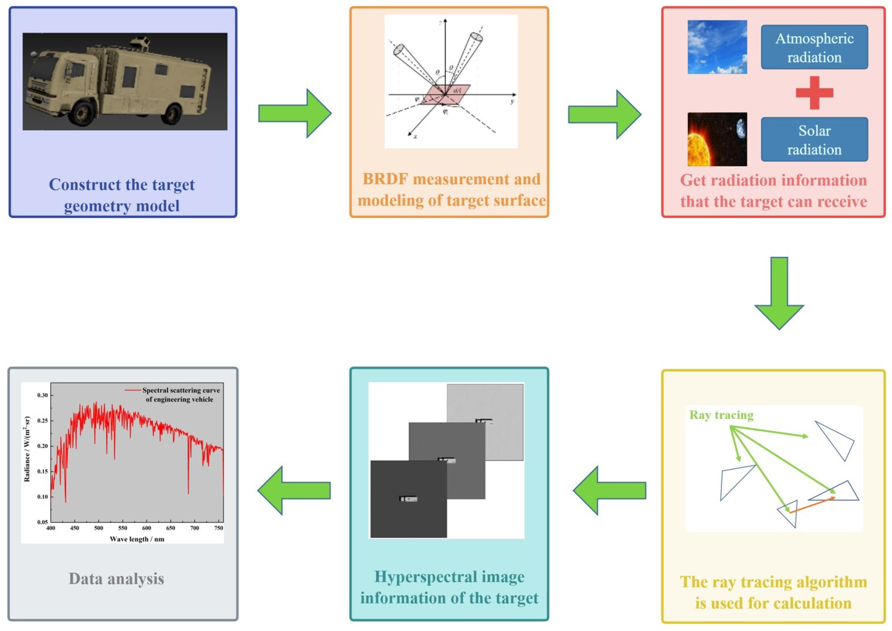
Figure 2.
Simulation flow of ray-tracing method.

Figure 3.
Ray occlusion and intersection judgment.

Figure 4.
Sampling method: (a) Random sampling of secondary scattered rays in hemispherical space; (b) The secondary scattered rays are sampled in the cone angle near the specular reflection direction.
Figure 4.
Sampling method: (a) Random sampling of secondary scattered rays in hemispherical space; (b) The secondary scattered rays are sampled in the cone angle near the specular reflection direction.

Figure 5.
The spectrum BRDF of spray paint in different colors: (a) white spray paint; (b) black spray paint; (c) gray-green paint; (d) gray paint.
Figure 5.
The spectrum BRDF of spray paint in different colors: (a) white spray paint; (b) black spray paint; (c) gray-green paint; (d) gray paint.

Figure 6.
Calculation results of solar irradiance.

Figure 7.
Calculated results of atmospheric radiation.

Figure 8.
A schematic of the simulated scene.

Figure 9.
Geometric model of grassland. (a) Grid plane. (b) Model representation.

Figure 10.
Geometric model of the scene. (a) Engineering vehicle model. (b) The engineering vehicle is on the grass.
Figure 10.
Geometric model of the scene. (a) Engineering vehicle model. (b) The engineering vehicle is on the grass.

Figure 11.
Coordinate system of scene.

Figure 12.
Visible light scattering image: zenith angle = 0; azimuth angle = 90.

Figure 13.
Visible light scattering images: (a) zenith angle = 30, azimuth angle = 90; (b) zenith angle = 45, azimuth angle = 90; (c) zenith angle = 60, azimuth angle = 90.
Figure 13.
Visible light scattering images: (a) zenith angle = 30, azimuth angle = 90; (b) zenith angle = 45, azimuth angle = 90; (c) zenith angle = 60, azimuth angle = 90.

Figure 14.
Visible light scattering images: (a) zenith angle = 45, azimuth angle = 0; (b) zenith angle = 45, azimuth angle = 90.
Figure 14.
Visible light scattering images: (a) zenith angle = 45, azimuth angle = 0; (b) zenith angle = 45, azimuth angle = 90.

Figure 15.
Visible light scattering images: (a) zenith angle = 45, azimuth angle = 180; (b) zenith angle = 45, azimuth angle = 270.
Figure 15.
Visible light scattering images: (a) zenith angle = 45, azimuth angle = 180; (b) zenith angle = 45, azimuth angle = 270.

Figure 16.
Visible light scattering images: (a) gray-green paint; (b) white paint.
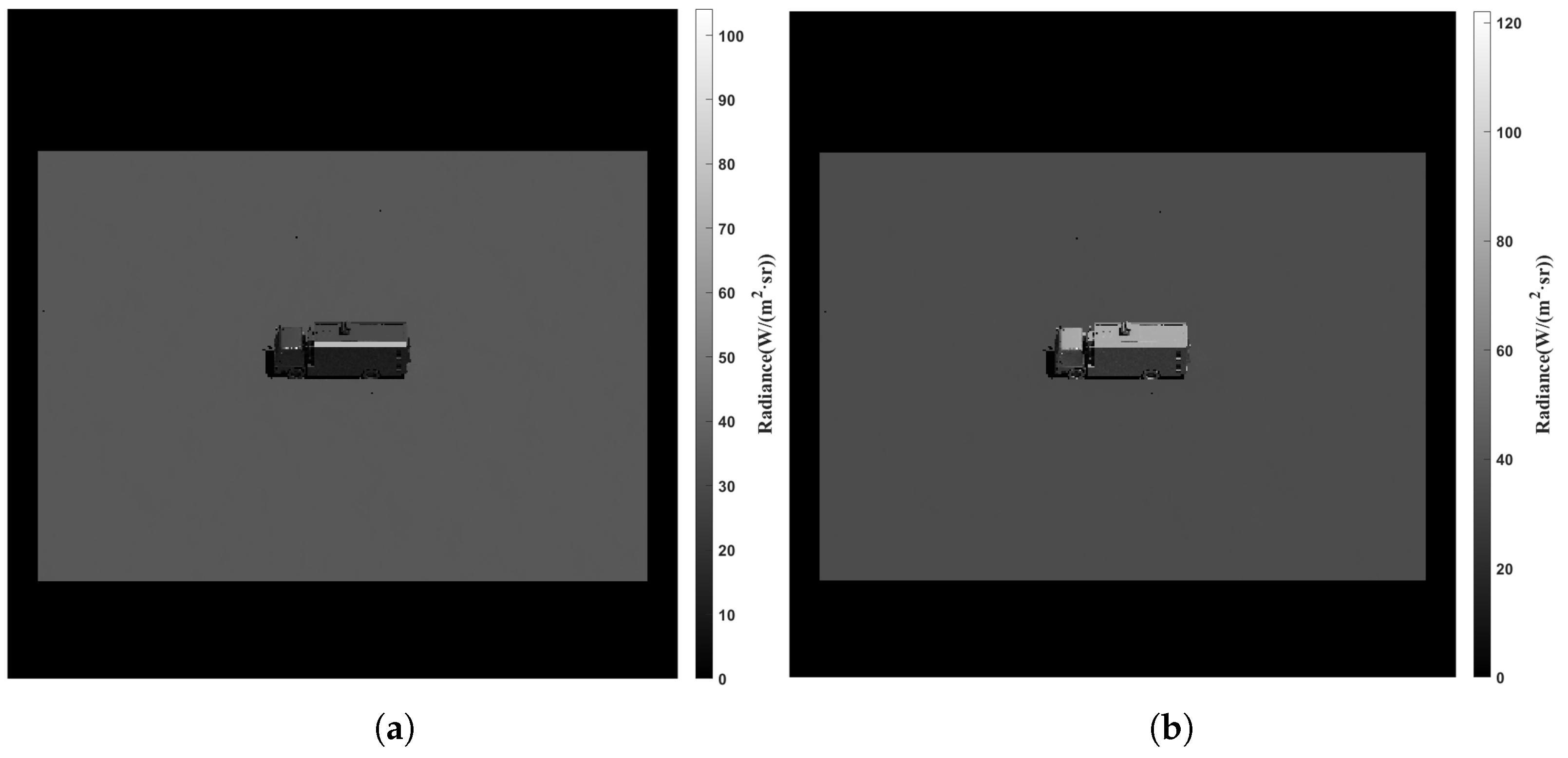
Figure 17.
The location of spectral data extraction.

Figure 18.
Spectral curves: (a) spectral scattering curve of white paint; (b) spectral scattering curve of gray-green paint.
Figure 18.
Spectral curves: (a) spectral scattering curve of white paint; (b) spectral scattering curve of gray-green paint.

Figure 19.
Comparison of scattering images at various wavelengths: (a) wavelength 430 nm, white paint; (b) wavelength 560 nm, white paint; (c) wavelength 720 nm, white paint; (d) wavelength 430 nm, gray-green paint; (e) wavelength 560 nm, gray-green paint; (f) wavelength 720 nm, gray-green paint.
Figure 19.
Comparison of scattering images at various wavelengths: (a) wavelength 430 nm, white paint; (b) wavelength 560 nm, white paint; (c) wavelength 720 nm, white paint; (d) wavelength 430 nm, gray-green paint; (e) wavelength 560 nm, gray-green paint; (f) wavelength 720 nm, gray-green paint.

Figure 20.
Comparison of the results of solar scattering, multiple scatterings, and atmospheric scattering: (a) solar scattering; (b) multiple scatterings; (c) scattering of atmospheric radiation.
Figure 20.
Comparison of the results of solar scattering, multiple scatterings, and atmospheric scattering: (a) solar scattering; (b) multiple scatterings; (c) scattering of atmospheric radiation.


Table 1.
The five parameters of the spectral BRDF for white paint.
| Wavelength (nm) | b | a | |||
|---|---|---|---|---|---|
| 400 | |||||
| 401 | |||||
| … | … | … | … | … | … |
| … | … | … | … | … | … |
| 759 | |||||
| 760 |
Table 2.
The BRDF encompasses three parameters specific to grassland.
| Core Weight | Band1 | Band2 | Band3 | Band4 |
|---|---|---|---|---|
Disclaimer/Publisher’s Note: The statements, opinions and data contained in all publications are solely those of the individual author(s) and contributor(s) and not of MDPI and/or the editor(s). MDPI and/or the editor(s) disclaim responsibility for any injury to people or property resulting from any ideas, methods, instructions or products referred to in the content. |
© 2024 by the authors. Licensee MDPI, Basel, Switzerland. This article is an open access article distributed under the terms and conditions of the Creative Commons Attribution (CC BY) license (https://creativecommons.org/licenses/by/4.0/).
Share and Cite
MDPI and ACS Style
Cao, Y.; Cao, Y.; Wu, Z.; Yang, K. A Calculation Method for the Hyperspectral Imaging of Targets Utilizing a Ray-Tracing Algorithm. Remote Sens. 2024, 16, 1779. https://doi.org/10.3390/rs16101779
AMA Style
Cao Y, Cao Y, Wu Z, Yang K. A Calculation Method for the Hyperspectral Imaging of Targets Utilizing a Ray-Tracing Algorithm. Remote Sensing. 2024; 16(10):1779. https://doi.org/10.3390/rs16101779
Chicago/Turabian StyleCao, Yisen, Yunhua Cao, Zhensen Wu, and Kai Yang. 2024. "A Calculation Method for the Hyperspectral Imaging of Targets Utilizing a Ray-Tracing Algorithm" Remote Sensing 16, no. 10: 1779. https://doi.org/10.3390/rs16101779
Note that from the first issue of 2016, this journal uses article numbers instead of page numbers. See further details here.