
Fractional-Order Least-Mean-Square-Based Active Control for an Electro–Hydraulic Composite Engine Mounts


1
School of Mechanical and Vehicle Engineering, Hunan University, Changsha 410082, China
2
Zhuzhou Times New Material Technology Co., Ltd., Zhuzhou 412000, China
*
Author to whom correspondence should be addressed.
Electronics 2024, 13(10), 1974; https://doi.org/10.3390/electronics13101974
Submission received: 18 April 2024
/
Revised: 15 May 2024
/
Accepted: 16 May 2024
/
Published: 17 May 2024
(This article belongs to the Special Issue Control and Optimization of Power Converters and Drives)
Abstract
:For the vibration of automobile powertrain, this paper designs electro–hydraulic composite engine mounts. Subsequently, the dynamic characteristics of the hydraulic mount and the electromagnetic actuator were analyzed and experimentally studied separately. Due to the strong nonlinearity of the hybrid electromechanical engine mount, a Fractional-Order Least-Mean-Square (FGO-LMS) algorithm was proposed to model its secondary path identification. To validate the vibration reduction effect, a rapid control prototype test platform was established, and vibration active control experiments were conducted based on the Multiple–Input Multiple–Output Filter-x Least-Mean-Square (MIMO-FxLMS) algorithm. The results indicate that, under various operating conditions, the vibration transmitted to the chassis from the powertrain was significantly suppressed.
1. Introduction
The powertrain system typically consists of an engine and a transmission, with the engine remaining one of the most widely used power sources in passenger vehicles and a primary source of vibration [1]. With the advancement of energy-saving and emission-reducing technologies, the vibration characteristics of engines have become increasingly complex [2]. Traditional hydraulic mounts possess functions such as isolation, support, and restraint, but they suffer from an inability to adapt to varying vibrations [3]. Active vibration isolation involves generating additional forces to counteract vibrations, allowing for adaptation to changing conditions and achieving optimal vibration reduction at all times. However, it faces challenges such as weak load-bearing capacity and high energy consumption [4]. Electro–hydraulic composite engine mounts integrate the technical advantages of both traditional and active systems [5], making them the optimal solution to address this challenge.
Further research is essential to optimize the comprehensive performance of electro–hydraulic composite engine mounts, including high load-carrying capacity, large active force, and high vibration isolation rate [6]. Freudenberg initially applied electromagnetic active mounts to FWD four-cylinder engine and achieved favorable vibration isolation results [7]. The actuator is a pivotal component of electro–hydraulic composite engine mounts, and the electromagnetic actuator is divided into the moving coil type and solenoid type according to the different moving parts [8]. Mansour et al. proposed a kind of active engine mounts based on electromagnetic actuator, where the design connects the electromagnetic actuator to the decoupling membrane of the liquid resistance mounts, establishing the fundamental framework of electro–hydraulic composite engine mounts [9]. Nevertheless, there is room for further improvement in the performance of electromagnetic actuators, including miniaturization, weight reduction, enhanced output force, and linearity of force output.
However, establishing an accurate system model for the active vibration control of powertrains is a formidable challenge [10]. FxLMS algorithms are based on the assumptions that the secondary path is a sliding average processes and random input signals, which avoids the dependence on an accurate system model, and thus has been widely studied in the field [11,12]. Here, the secondary path refers to the electro–hydraulic composite engine mounts as the main one, and also includes the sensors and controller, including the entire control signaling channel, which is highly time-varying and affected by multiple parameters such as temperature [13,14]. However, there is room for improvement in the transient and steady-state characteristics of this algorithm [15], especially when the phase error between the secondary path and its estimated value exceeds 90°, which may lead to serious performance degradation [11]. Therefore, Hillis reduces the interference of noise by means of frequency domain blocks, which effectively reduces the transmission of engine vibration to the body, but the transient performance of the algorithm is degraded [16]. Yang Q et al. introduced the wavelet packet decomposition algorithm with the Hartley block least-mean-square algorithm for improving the convergence speed of the FxLMS algorithm at a stable frequency, but it is difficult to satisfy the working conditions with frequent frequency changes [17]. Guo R et al. proposed an acceleration-extended FxLMS for active control of powertrain vibration and conducted simulation studies to prove its effectiveness, but did not conduct further experimental studies [18]. Tang and Hong controlled the engine vibration by NLMS algorithm, but the effect is nearly the same as the classical FxLMS [19,20]. Jia put forward a kind of hybrid PI-FxLMS control algorithm to control the engine vibration, but the vibration controlling effect is not improved greatly when the reference signal is not in disturbance [21]. Hauserg et al. interpolated the secondary path model into a table for querying by the FxLMS algorithm, which can greatly simplify the computation, but the accuracy of the model is difficult to guarantee [22]. In summary, it is very meaningful to study electro–hydraulic composite engine mounts and powertrain vibration active control algorithms to reduce the vibration and noise of automobiles caused by the powertrain.
Therefore, this paper designs an electromagnetic–hydraulic composite engine mounts based on a specific test model and conducts modeling and analysis. It utilizes fractional-order gradient descent to optimize the LMS algorithm for secondary path identification, considering the nonlinear characteristics of the actuator in the electro–hydraulic composite engine mounts system. Finally, a test platform based on the actual vehicle powertrain is established, and rapid control prototype tests for vibration active control are conducted using the MIMO-FxLMS algorithm. The results indicate a significant suppression of vibrations transmitted to the subframe under various powertrain operating conditions.
2. Electro–Hydraulic Composite Engine Mounts
2.1. Mounts Dynamics Analysis
The electro–hydraulic composite engine mounts system consists of an electromagnetic actuator and rubber hydraulic mounts. When the actuator is not operating, the passive part of the electro–hydraulic composite suspension has similar characteristics to the original rubber hydraulic suspension, in which a conical spring providing power assembly support and acting as a piston in the main chamber. At low-frequency large displacements, the compression of the spring forces the liquid in the main chamber to enter the compensation chamber through the damping channel to form damping and realize passive vibration isolation. At high-frequency small displacements, the liquid is hard to pass through the damping channel quickly, but the decoupling membrane is deformed to compensate for the volume change. At this time, the electromagnetic actuator will output a force, which is the opposite phase of the actuating force, and the active vibration isolation could be obtained. This combines the advantages of active and passive to realize composite vibration isolation. The equivalent mechanical model of the active mounts is shown in Figure 1, representing a lumped-parameter model.
Where the following are defined: Br—equivalent damping coefficient of rubber main spring, Ns/m; Kr—equivalent stiffness coefficient of rubber main spring, N/m; Ap—equivalent piston area of rubber main spring, m2; C1—volumetric flexibility of the upper liquid chamber, m5/N; C2—volumetric flexibility of the lower liquid chamber, m5/N; Ad—area of the vibrating membrane, m2; Kd—vibrating membrane stiffness, N/m; Qi—flow rate of inertial channel, m3/s; Ri—liquid resistance of inertial channel, kg/m4s; Ii—fluid inductance of inertial channel, kg/m4; Fa—electromagnetic actuator actuation force on the vibrating membrane, N; x—equivalent displacement of the rubber main spring, m; xd—displacement of the vibrating membrane, m; P1—upper liquid chamber pressure, Pa; P2—lower liquid chamber pressure, Pa.
The above lumped parameters are used to model the lumped parameters of the active mount device.
The continuity equation of the liquid in the upper liquid chamber of the mount is given by:
The continuity equation of the liquid in the lower liquid chamber of the mount is:
The equilibrium equation of motion of the fluid in the inertial channel is:
The equilibrium equation of motion of the vibrating membrane is:
The force transferred to the mounting base by the active mounts is:
According to the above analysis, we can see that the active force Fa was considered as an independent parameter in the electro–hydraulic composite suspension. The design of the liquid suspension part can still be carried out according to the classical theory. Therefore, a hydraulic suspension product that we have already mass-produced was chosen as an input with the core parameters shown in Table 1, which matches the test vehicle in this paper.
2.2. Linear Electromagnetic Actuator
The linear electromagnetic actuator mainly consists of a fixed coil and a moving core (comprising several magnets and connecting rods, etc.). The structure of the linear electromagnetic actuator is illustrated in Figure 4.
The alternating current generates an alternating magnetic field through the coil, which interacts with the permanent magnet, resulting in the output of Lorentz magnetic force through the connecting rod. The ends of the connecting rod are connected to springs, which are displaced by the electromagnetic force, thus providing a restoring force for the actuator. According to [23], the Lorentz magnetic force is a function of the change in current and is expressed as:
where is the residual flux density of the permanent magnet, is the air permeability, I is the current, is the leakage coefficient, is the air gap width, h is the height of the air gap, l is the height of the permanent magnet, is the outer diameter of the actuator, is the thickness of the permanent magnet, is the AC circuit reluctance, and is the magnetic resistance of the permanent.
To match the active vibration control system, the actuator requires the force output maximum, size, resonant frequency, and so on. To satisfy the requirement of the actuator, we set the main parameters of the electromagnetic actuator (shown in Table 2) independently, according to the theory of electromagnetism.
The electromagnetic force of the actuator is tested under three working conditions of 1 A, 2 A, and 12 V, respectively, and the frequency range is 10–250 Hz, and the test setup is shown in Figure 5. The results, as shown in Figure 6a, indicate that the electromagnetic force is inversely proportional to the square of the magnetic circuit reluctance. Therefore, under the 12 V condition, as the frequency increases, the inductive reactance gradually increases, leading to a gradual decrease in the electromagnetic force, but the rate of decrease gradually slows down. Plotting the specific current force in Figure 6b, the current is 1 A and 2 A at each frequency than the current force is almost the same; i.e., the electromagnetic force and the current is basically a linear relationship.
3. FGO-LMS Algorithm and Secondary Path Identification
Fractional-order differentiation can more accurately describe nonlinear dynamic behaviors and complex phenomena [24]. Considering the strong nonlinearity characterizing the secondary path, it is proposed to use the fractional-order differentiation gradient descent method to replace the traditional first-order differentiation. The block diagram of this algorithm is shown in Figure 7.
Where x(n) is the excitation signal in the recognition process, S(z) is the actual secondary path to be recognized, WS(z) is the simulated secondary path recognized by the adaptive algorithm, and e(n) is the residual error signal. Let WS(z) weight vector be , M be the filter length, and be the input vector.
The weight vector update formula is:
where the objective function expression J(n) is:
Therefore, the weight vector update equation in Equation (8) is transformed as:
Replacing the integer-order gradient of Equation (8) with a fractional-order gradient:
Introducing the fractional-order gradient descent method here, according to [26], the expression for the fractional-order gradient descent of the objective function can be obtained as:
where the values of are very small and can be ignored. At the same time, will be replaced in the form of the L2 paradigm, so the final FGO-LMS algorithm for updating the weight vector is given by:
where is the algorithm order, which takes values in the range (0,1):
During the secondary path identification, the electro–hydraulic composite engine mount was installed on the vehicle, and then the white noise signal was input to the actuator of the engine mount and the signal of sensor on the engine mount was obtained as the response. The secondary path could be calculated by computer program using the fractional-order LMS and classical LMS algorithms after the excitation and response obtained. The evaluation criteria primarily includes convergence performance and steady-state misalignment performance. Convergence speed characterizes the algorithms’ ability to accurately track changes in weight coefficients in a non-stationary environment, while steady-state misalignment performance characterizes the minimum mean-square error that still exists when weight coefficients converge to their optimal values. Both algorithms have a step size of 10−5 and a filter length of 128 orders. The fractional-order LMS algorithm orders were set as 0.1, 0.3, 0.5, 0.7, and 0.9, respectively. Figure 8 presents a performance comparison of the two algorithms. It is evident that when the fractional-order is set to 0.9, it converges with the fewest iterations and exhibits lower steady-state error, indicating that fractional-order LMS can indeed provide a more accurate characterization of the secondary path.
4. MIMO-FxLMS Algorithm and Active Vibration Control Test
4.1. MIMO-FxLMS Active Vibration Control
The test platform shown in Figure 9 consists of an electro–hydraulic composite engine mounts, a vehicle equipped with a V4 engine and a dSPACE, and the main structure of the system is shown in Figure 10. At the front of the powertrain, there is an active mount arranged on both left and right sides, the acceleration signal at its lower end, the connection point with the subframe, is input as an error signal.
Therefore, the MIMO-FXLMS algorithm, designed in conjunction with the powertrain active vibration control system, is shown in Figure 11.
Where the engine vibration passes through the primary path to become , which is the offsetting vibration, is the secondary path, and is the identification model, also known as the secondary path filter shown in Equation (16), obtained from the fractional-order gradient descent LMS identification designed in Section 3. The control signal passing through the becomes , which is actuated and used to offset the .
After the reference signal is filtered by the secondary path, the filtered reference signal is obtained as:
The iterative equation for the MIMO-FxLMS system weights is:
where and represent the left and right channel weights, respectively, , , and are the reference signal of different channels, and is the step size.
Ultimately, the actuator drive voltage is calculated as:
4.2. Test and Result
The error sensors in the system are installed near the mounting points of the electro–hydraulic composite engine mounts, allowing the use of multiple independent secondary path filters to locally minimize each error signal. Tests were carried out under two typical operating conditions, idling and setup rise, and compared with the results of the tests with no control.
The time-domain signal comparison of the left and right error sensor signals under idling conditions is shown in Figure 12, where the self-power spectrum is obtained for the frequency-domain signal comparison, and the engine speed under idling conditions is 700~750 rpm; that is, the second-order vibration frequency is 23.3~25 Hz. And the self-power spectrum in the corresponding vibration frequency range is obtained as shown in Figure 13, where the second-order vibration is reduced by 18.12 dB in the left error sensor by the MIMO-FxLMS algorithm compared to that with no control. At the left error sensor, the MIMO-FxLMS algorithm reduces the second-order vibration by 18.12 dB compared with no control, and at the right error sensor, the MIMO-FxLMS algorithm reduces the second-order vibration by 10.33 dB compared with no control, which is a significant vibration suppression effect.
Comparison of the vibration situation in the fixed rise condition: The time-domain vibration acceleration signals at the left and right error sensor locations, collected throughout the engine’s acceleration from idle to 4000 rpm, are shown in Figure 14, and the different time durations in the two sets are due to the manual control of the throttle by the driver during testing, making it difficult to achieve complete consistency.
The time-domain signals near different rotational speeds are further extracted, and their derived self-power spectra are compared, as shown in Figure 15, Figure 16, Figure 17, Figure 18, Figure 19 and Figure 20, where the relationship between the frequency of the second-order vibration and the rotational speed is shown as:
where f2nd represents the frequency of the second-order vibration, whose unit is Hz, and RPM represents the rotational speed, whose unit is rpm (revolutions per minute).
When the rotational speed is 1500 rpm, the vibration level at the left error sensor is −24.92 dB and the vibration level at the right error sensor is −39.36 dB with no control; when using the MIMO-FxLMS algorithm for control, the vibration level at the left error sensor location is −37.21 dB, and at the right error sensor location, it is −47.47 dB.
When the rotational speed is 2000 rpm, with no control, the left error sensor is −20.33 dB and the right error sensor is −41.33 dB, while the left error sensor is −35.60 dB and the right error sensor is −43.54 dB when the MIMO-FxLMS algorithm is utilized.
When the speed is 2500 rpm, the vibration level at the left error sensor is −12.16 dB with no control, the vibration level at the right error sensor is −33.88 dB, and the vibration level at the left error sensor is −23.40 dB with the MIMO-FxLMS algorithm, and the vibration level at the right error sensor is −36.41 dB.
When the speed is 3000 rpm, the vibration level at the left error sensor is −15.47 dB with no control, and the vibration level at the right error sensor is −33.92 dB. When the speed is 3000 rpm, the vibration level is −20.95 dB at the left error sensor and −38.37 dB at the right error sensor when the vibration is controlled.
When the speed is 3500 rpm, the vibration level is −17.34 dB at the left error sensor and −35.39 dB at the right error sensor with no control; when the speed is 3500 rpm, the vibration level is −20.35 dB at the left error sensor and −38.80 dB at the right error sensor when the vibration is controlled.
At 4000 rpm, the vibration level at the left error sensor is −14.45 dB, the vibration level at the right error sensor is −26. 71 dB with no control, and the vibration level at the left error sensor is −19.03 dB, and the vibration level at the right error sensor is −28.89 dB using the MIMO-FxLMS algorithm.
5. Results
- (1)
- In this paper, an electro–hydraulic engine mount was designed, and the dynamic stiffness was measured under different loads, which showed that the dynamic stiffness of the hydraulic engine mount will increase as the frequency of load increases. For example, when the loaded displacement is ±1 mm, the dynamic stiffness of the hydraulic engine mount is nearly 500 N/mm at a high frequency, while it is 200 N/mm at a low frequency. Meanwhile, the electromagnetic force output test of the actuator was taken, which showed that the electromagnetic force output was linear to the current.
- (2)
- In this paper, the secondary path identification using the FGO-LMS algorithm was taken. As the results showed, the FGO-LMS could converge at nearly 5000 iterations, while the classical LMS converges at nearly 9000 iterations, and the mean square error (MSE) is nearly 0.025 when the FGO-LMS converges, while the MSE is nearly 0.031 when the classical LMS converges.
- (3)
- In this paper, an active vibration control experiment was performed. As the results showed, the vibration level of the left sensor decreased by 18 dB, while the vibration level of the right sensor decreased by 10 dB when the MIMO-LMS algorithm was used to control the vibration of engine at idle conditions. And the MIMO-LMS algorithm could also control the vibration effectively at different rotational engine speeds. As the experiment results showed, the vibration level at the left sensor decreased by 12.29 dB/15.27 dB/11.24 dB/5.48 dB/3.01 dB/4.58 dB, respectively, at 1500 rpm/2000 rpm/2500 rpm/3000 rpm/3500 rpm/4000 rpm, while the vibration level at the right sensor decreased by 8.11 dB/2.21 dB/2.53 dB/4.45 dB/3.41 dB/2.18 dB, respectively.
6. Conclusions
- (1)
- Based on the active vibration reduction requirements of a test vehicle powertrain, an electro–hydraulic composite engine mount was designed, and its electromagnetic actuator and rubber hydraulic mounts were dynamically analyzed and tested;
- (2)
- A FGO-LMS algorithm was proposed based on the nonlinear characteristics of the electro–hydraulic composite engine mounts, and based on this, the secondary path was identified, which improved the convergence speed and steady-state characteristics compared to classical LMS;
- (3)
- Based on the MIMO-FxLMS algorithm, active vibration control experiments were conducted, and the results showed that the electro–hydraulic composite engine mounts used had a vibration attenuation of 18 dB and 10 dB for the left and right sides under idle conditions, respectively, demonstrating their excellent vibration suppression effect within the frequency range of concern under fixed rising working conditions.
- (4)
- In the future, the active vibration control using the FGO-LMS algorithm with online secondary path identification will be studied in great depth. And the MIMO-FxLMS algorithm could be expanded to a Multi-order MIMO-FxLMS algorithm, which is used to control different order vibrations at the same time. Meanwhile, the FGO-LMS algorithm might be used to improve the active vibration control effect when the car is on the road.
Author Contributions
Conceptualization, L.W. and J.Y.; methodology, L.W. and X.D.; software, X.D.; validation, L.W.; resources, J.Y.; writing—original draft, L.W.; writing—review & editing, R.D. and K.L.; visualization, R.L.; supervision, R.D. and K.L. All authors have read and agreed to the published version of the manuscript.
Funding
This research was funded by the Science and Technology Innovation Program of Hunan Province, grant number 2021RC4027.
Data Availability Statement
Data is contained within the article.
Conflicts of Interest
Author Jun Yang and Xingwu Ding were also employed by Zhuzhou Times New Material Technology Co., Ltd. The remaining authors declare that the research was conducted in the absence of any commercial of financial relationships that could be construed as a potential conflict of interest.
References
- Qin, Y.; Tang, X.; Jia, T.; Duan, Z.; Zhang, J.; Li, Y.; Zheng, L. Noise and vibration suppression in hybrid electric vehicles: State of the art and challenges. Renew. Sustain. Energy Rev. 2020, 124, 109782. [Google Scholar] [CrossRef]
- Yu, Y.; Naganathan, N.G.; Dukkipati, R.V. A literature review of automotive vehicle engine mounting systems. Mech. Mach. Theory 2001, 36, 123–142. [Google Scholar] [CrossRef]
- Römling, S.; Vollmann, S.; Kolkhorst, T. Active engine mount system in the new Audi S8. MTZ Worldw. 2013, 74, 34–38. [Google Scholar] [CrossRef]
- Kim, S.H.; Park, U.H.; Kim, J.H. Voice Coil Actuated engine mount for vibration reduction in automobile. Int. J. Automot. Technol. 2020, 21, 771–777. [Google Scholar] [CrossRef]
- Raoofy, A.; Fakhari, V.; Ohadi Hamedani, A.R. Vibration control of an automotive engine using active mounts. Engine Res. 2022, 30, 3–14. [Google Scholar]
- Li, D.; He, Q.; Yan, Z.; Li, X. Design of a linear electromagnetic actuator for active vibration control. In Proceedings of the 2018 3rd International Conference on Mechanical, Control and Computer Engineering (ICMCCE), Huhhot, China, 14–18 September 2018; pp. 21–25. [Google Scholar]
- Birch, S. Vibration. USA Automot. Eng. 1988, 2, 56–60. [Google Scholar]
- Swanson, D.A. Active Engine Mounts for Vehicles; SAE Technical Paper: Warrendale, PA, USA, 1993. [Google Scholar]
- Mansour, H.; Arzanpour, S.; Golnaraghi, F. Design of a solenoid valve based active engine mount. J. Vib. Control. 2012, 18, 1221–1232. [Google Scholar] [CrossRef]
- Fan, R.L.; Wang, P.; Han, C.; Wei, L.J.; Liu, Z.J.; Yuan, P.J. Summarisation, simulation and comparison of nine control algorithms for an active control mount with an oscillating coil actuator. Algorithms 2021, 14, 256. [Google Scholar] [CrossRef]
- Cheng, Y.; Ge, P.; Chen, S.; Li, C.; Jiang, Y. A novel multi-gradient direction FxLMS algorithm with output constraint for active noise control. In INTER-NOISE and NOISE-CON Congress and Conference Proceedings, Lexington, KY, USA, 13–15 June 2022; Institute of Noise Control Engineering: Wakefield, MA, USA; Volume 264, pp. 951–962.
- Zhang, H.; Shi, W. Model of the secondary path between the input voltage and the output force of an active engine mount on the engine side. Math. Probl. Eng. 2020, 2020, 1–16. [Google Scholar] [CrossRef]
- Guo, R.; Wei, X.K.; Zhou, S.Q.; Gao, J. Parametric identification study of an active engine mount: Combination of finite element analysis and experiment. Proc. Inst. Mech. Eng. Part D J. Automob. Eng. 2019, 233, 427–439. [Google Scholar] [CrossRef]
- Han, C.; Serra, Q.; Laurent, H.; Florentin, É. Parameter Identification of Fractional Order Partial Differential Equation Model Based on Polynomial–Fourier Method. Int. J. Appl. Comput. Math. 2024, 10, 1–26. [Google Scholar] [CrossRef]
- Song, P.; Zhao, H. Filtered-x least mean square/fourth (FXLMS/F) algorithm for active noise control. Mech. Syst. Signal Process. 2019, 120, 69–82. [Google Scholar] [CrossRef]
- Hillis, A.J. Multi-input multi-output control of an automotive active engine mounting system. Proc. Inst. Mech. Eng. Part D J. Automob. Eng. 2011, 225, 1492–1504. [Google Scholar] [CrossRef]
- Yang, Q.; Ma, Z.; Zhou, R. A Two-DOF Active-Passive Hybrid Vibration Isolator Based on Multi-Line Spectrum Adaptive Control. Machines 2022, 10, 825. [Google Scholar] [CrossRef]
- Guo, R.; Wei, X.K.; Gao, J. Extended filtered-x-least-mean-squares algorithm for an active control engine mount based on acceleration error signal. Adv. Mech. Eng. 2017, 9, 1687814017724350. [Google Scholar] [CrossRef]
- Tang, Y.; Wang, L.; Wu, X.; Liu, S.; Zhang, Q. Simulation of Active Engine Suspension Vibration Control Based on Momentum NLMS Algorithm. Ind. Control. Comput. 2023, 36, 19–21. [Google Scholar]
- Hong, D.; Moon, H.; Kim, B. Feasibility study on the active structural attenuation of multiple band vibrations from two dimensional continuous structures in automotive vehicles. Adv. Mech. Eng. 2024, 16, 16878132241243170. [Google Scholar] [CrossRef]
- Jia, Q.; Li, Q.; Liu, L. Sufficient active control of uncertain low-frequency space micro-vibrations near measurement limit of acceleration sensors. Aerosp. Sci. Technol. 2024, 12, 109136. [Google Scholar] [CrossRef]
- Hausberg, F.; Plöchl, M.; Rupp, M.; Pfeffer, P.; Hecker, S. Combination of map-based and adaptive feedforward control algorithms for active engine mounts. J. Vib. Control. 2017, 23, 3092–3107. [Google Scholar] [CrossRef]
- Zhang, Q.W.; Yu, X.; Yan, Z.T.; Yang, H.L. Dynamic characteristics and algorithm of an electromagnetic-hydraulic active-passive vibration isolator. J. Vib. Eng. 2022, 35, 417–425. [Google Scholar]
- Li, T.; Wang, N.; He, Y.; Xiao, G.; Gui, W.; Feng, J. Noise cancellation of a train electric traction system fan based on a fractional-order variable-step-size active noise control algorithm. IEEE Trans. Ind. Appl. 2022, 59, 2081–2090. [Google Scholar] [CrossRef]
- Yin, K.L.; Zhao, H.R.; Pu, Y.F.; Lu, L. Nonlinear active noise control with tap-decomposed robust volterra filter. Mech. Syst. Signal Process. 2024, 206, 110887. [Google Scholar] [CrossRef]
- Li, T.; Wang, M.; He, Y.; Wang, N.; Yang, J.; Ding, R.; Zhao, K. Vehicle engine noise cancellation based on a multi-channel fractional-order active noise control algorithm. Machines 2022, 10, 670. [Google Scholar] [CrossRef]
Figure 1.
Model diagram of the total parameters of the electro–hydraulic composite engine mounts.

Figure 2.
The stiffness testing of the electro–hydraulic engine mounts.
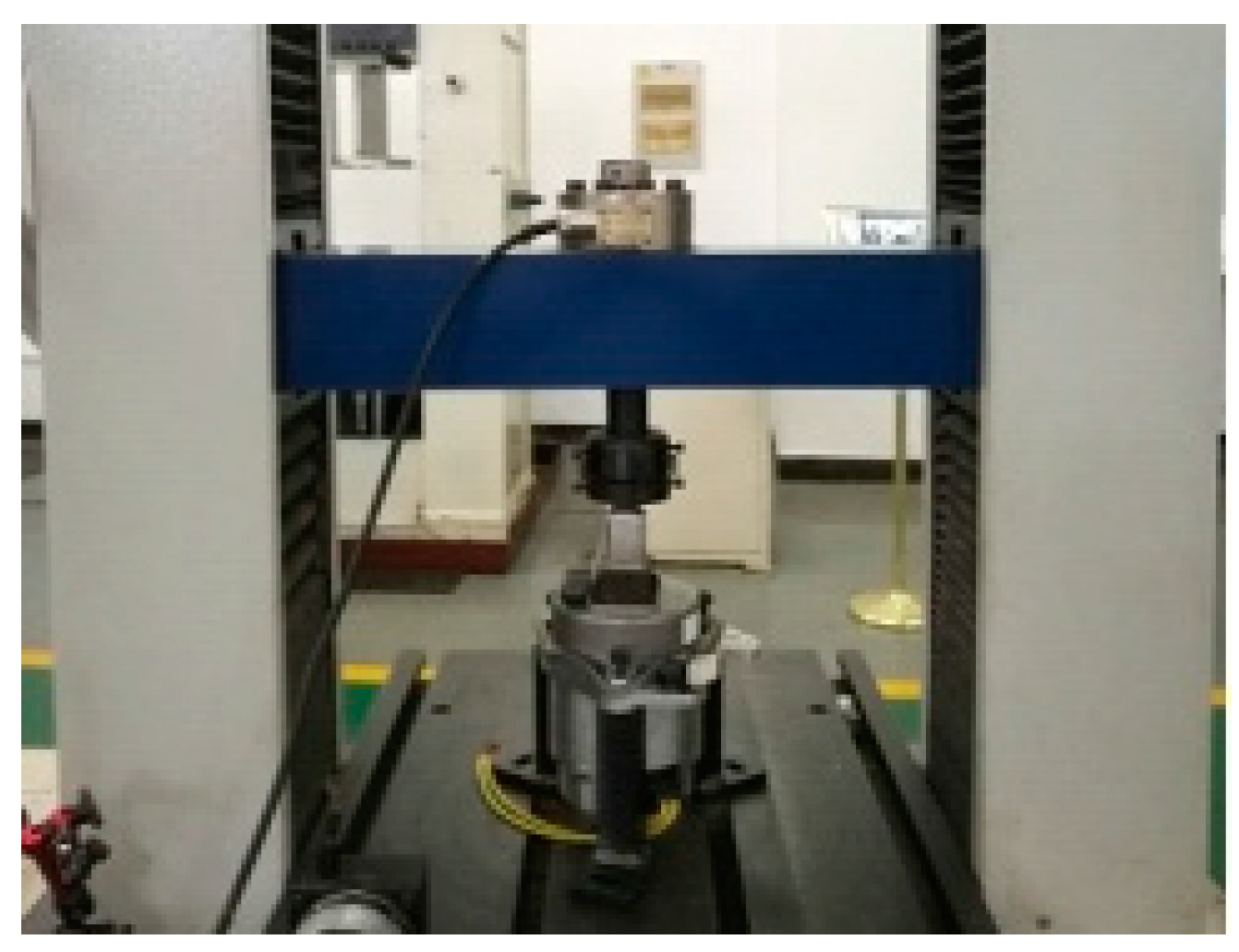
Figure 3.
Structural performance of active mounts. (a) Low-frequency dynamic stiffness and phase angle characteristics (loaded displacement ± 1 mm); (b) dynamic stiffness characteristics (loaded displacement ± 0.02 mm).
Figure 3.
Structural performance of active mounts. (a) Low-frequency dynamic stiffness and phase angle characteristics (loaded displacement ± 1 mm); (b) dynamic stiffness characteristics (loaded displacement ± 0.02 mm).
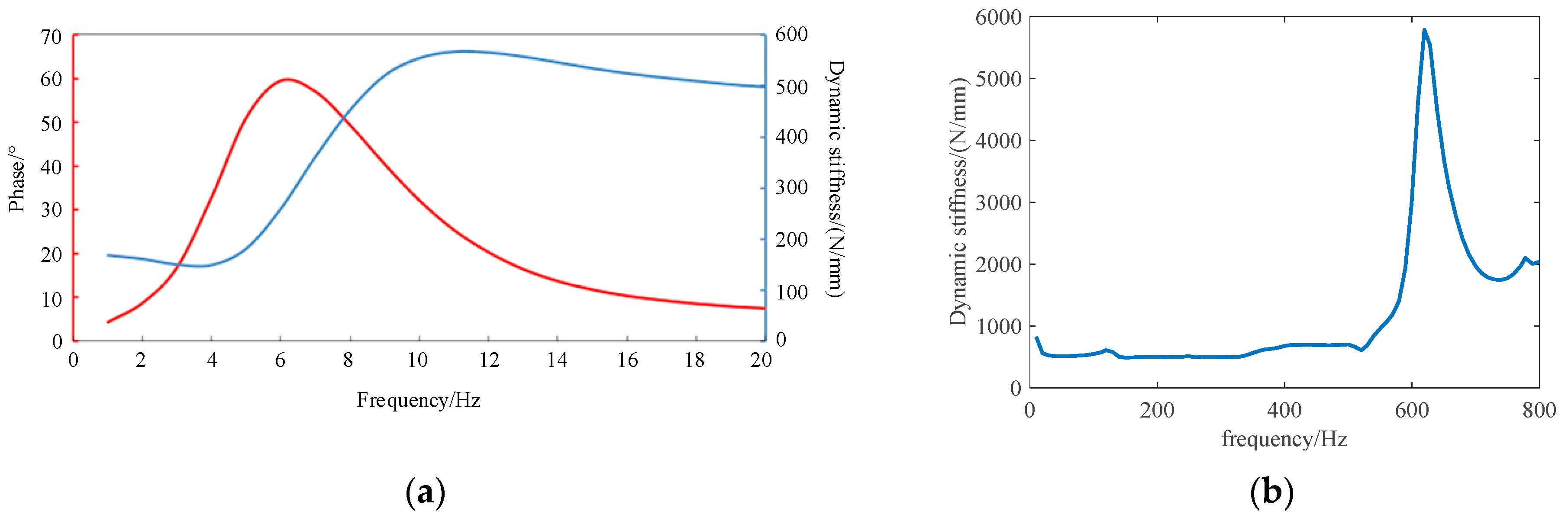
Figure 4.
Linear electromagnetic actuator structure. 1. Magnets; 2. armature; 3. connecting rod; 4. position tube; 5. carrier sheet; 6. spring; 7. transformers; 8. sleeve; 9. rotor; 10. wire.
Figure 4.
Linear electromagnetic actuator structure. 1. Magnets; 2. armature; 3. connecting rod; 4. position tube; 5. carrier sheet; 6. spring; 7. transformers; 8. sleeve; 9. rotor; 10. wire.

Figure 5.
Actuator test site diagram.

Figure 6.
Electromagnetic force. (a) Electromagnetic force output test results; (b) actuator current output comparison at different currents.
Figure 6.
Electromagnetic force. (a) Electromagnetic force output test results; (b) actuator current output comparison at different currents.

Figure 7.
Block diagram of fractional-order gradient descent LMS algorithm.

Figure 8.
Performance comparison of secondary path recognition algorithms. (a) Steady-state misalignment; (b) mean square error.
Figure 8.
Performance comparison of secondary path recognition algorithms. (a) Steady-state misalignment; (b) mean square error.

Figure 9.
Rapid control prototype test platform. (a) Subframe fitted with electro–hydraulic composite engine mounts; (b) modified test vehicle.
Figure 9.
Rapid control prototype test platform. (a) Subframe fitted with electro–hydraulic composite engine mounts; (b) modified test vehicle.

Figure 10.
Block diagram of the rapid control prototype test platform system.

Figure 11.
Block diagram of the MIMO-FxLMS active mounts control algorithm.

Figure 12.
Time-domain signals of sensors at idle conditions. (a) Left sensor; (b) right sensor.

Figure 13.
Self-power spectrum of sensor signals at idle conditions. (a) Left sensor; (b) right sensor.
Figure 13.
Self-power spectrum of sensor signals at idle conditions. (a) Left sensor; (b) right sensor.

Figure 14.
Time-domain signal at the fixed rise condition. (a) Left sensor; (b) right sensor.

Figure 15.
Self-power spectrum comparison of capturing speed under fixed rising conditions. (a) Autogram of left error sensor signal at 1500 rpm; (b) autogram of right error sensor signal at 1500 rpm.
Figure 15.
Self-power spectrum comparison of capturing speed under fixed rising conditions. (a) Autogram of left error sensor signal at 1500 rpm; (b) autogram of right error sensor signal at 1500 rpm.

Figure 16.
Self-power spectrum comparison of capturing speed under fixed rising conditions. (a) Autogram of left error sensor signal at 2000 rpm; (b) autogram of right error sensor signal at 2000 rpm.
Figure 16.
Self-power spectrum comparison of capturing speed under fixed rising conditions. (a) Autogram of left error sensor signal at 2000 rpm; (b) autogram of right error sensor signal at 2000 rpm.

Figure 17.
Self-power spectrum comparison of capturing speed under fixed rising conditions. (a) Autogram of left error sensor signal at 2500 rpm; (b) autogram of right error sensor signal at 2500 rpm.
Figure 17.
Self-power spectrum comparison of capturing speed under fixed rising conditions. (a) Autogram of left error sensor signal at 2500 rpm; (b) autogram of right error sensor signal at 2500 rpm.

Figure 18.
Self-power spectrum comparison of capturing speed under fixed rising conditions. (a) Autogram of left error sensor signal at 3000 rpm; (b) autogram of right error sensor signal at 3000 rpm.
Figure 18.
Self-power spectrum comparison of capturing speed under fixed rising conditions. (a) Autogram of left error sensor signal at 3000 rpm; (b) autogram of right error sensor signal at 3000 rpm.

Figure 19.
Self-power spectrum comparison of capturing speed under fixed rising conditions. (a) Autogram of left error sensor signal at 3500 rpm; (b) autogram of right error sensor signal at 3500 rpm.
Figure 19.
Self-power spectrum comparison of capturing speed under fixed rising conditions. (a) Autogram of left error sensor signal at 3500 rpm; (b) autogram of right error sensor signal at 3500 rpm.

Figure 20.
Self-power spectrum comparison of capturing speed under fixed rising conditions. (a) Autogram of left error sensor signal at 4000 rpm; (b) autogram of right error sensor signal at 4000 rpm.
Figure 20.
Self-power spectrum comparison of capturing speed under fixed rising conditions. (a) Autogram of left error sensor signal at 4000 rpm; (b) autogram of right error sensor signal at 4000 rpm.


Table 1.
Hydraulic mounts main parameters.
| No. | Parameter Name | Symbol | Value | Unit |
|---|---|---|---|---|
| 1 | Equivalent stiffness coefficient of a rubber main spring | Kr | 310 | N/mm |
| 2 | Equivalent damping coefficient for rubber main springs | Br | 0.1 | N.s/mm |
| 3 | Equivalent piston area of a rubber main spring | Ap | 4400 | mm2 |
| 4 | Volume flexibility of the upper liquid chamber | C1 | 31,079 | mm5/N |
| 5 | Volume flexibility of the lower liquid chamber | C2 | 2.6 × 10⁶ | mm5/N |
| 6 | Area of vibrating membrane | Ad | 2820 | mm2 |
| 7 | Diaphragm stiffness | Kd | 110 | N/mm |
| 8 | Decoupling membrane liquid sense | Ii | 2.16 × 10⁴ | kg/m4 |
| 9 | Decoupling membrane liquid resistance | Ri | 4.3 × 10⁷ | N.s/m5 |
Table 2.
Electromagnetic actuator main parameters table.
| No. | Parameter Name | Symbol | Value | Unit |
|---|---|---|---|---|
| 1 | Permanent magnet residual flux density | Bm | 1.5 | T |
| 2 | Number of turns | N | 60 | / |
| 3 | Air gap width | agap | 1 | mm |
| 4 | Outer diameter of actuator | dmov | 50 | mm |
| 5 | Height of permanent magnet | l | 13 | mm |
| 6 | Maximum amplitude | x | ±2 | mm |
| 7 | Spring stiffness | k | 110 | N/mm |
Disclaimer/Publisher’s Note: The statements, opinions and data contained in all publications are solely those of the individual author(s) and contributor(s) and not of MDPI and/or the editor(s). MDPI and/or the editor(s) disclaim responsibility for any injury to people or property resulting from any ideas, methods, instructions or products referred to in the content. |
© 2024 by the authors. Licensee MDPI, Basel, Switzerland. This article is an open access article distributed under the terms and conditions of the Creative Commons Attribution (CC BY) license (https://creativecommons.org/licenses/by/4.0/).
Share and Cite
MDPI and ACS Style
Wang, L.; Ding, R.; Liu, K.; Yang, J.; Ding, X.; Li, R. Fractional-Order Least-Mean-Square-Based Active Control for an Electro–Hydraulic Composite Engine Mounts. Electronics 2024, 13, 1974. https://doi.org/10.3390/electronics13101974
AMA Style
Wang L, Ding R, Liu K, Yang J, Ding X, Li R. Fractional-Order Least-Mean-Square-Based Active Control for an Electro–Hydraulic Composite Engine Mounts. Electronics. 2024; 13(10):1974. https://doi.org/10.3390/electronics13101974
Chicago/Turabian StyleWang, Lida, Rongjun Ding, Kan Liu, Jun Yang, Xingwu Ding, and Renping Li. 2024. "Fractional-Order Least-Mean-Square-Based Active Control for an Electro–Hydraulic Composite Engine Mounts" Electronics 13, no. 10: 1974. https://doi.org/10.3390/electronics13101974
Note that from the first issue of 2016, this journal uses article numbers instead of page numbers. See further details here.