Article

Sensitivity of a Process for Heating Thin Metal Film Described by the Dual-Phase Lag Equation with Temperature-Dependent Thermophysical Parameters to Perturbations of Lag Times

1
Department of Computational Mechanics and Engineering, Silesian University of Technology, Konarskiego 18a, 44-100 Gliwice, Poland
2
Department of Technical Sciences, University of Occupational Safety Management in Katowice, Bankowa 8, 42-200 Katowice, Poland
*
Author to whom correspondence should be addressed.
Energies 2024, 17(10), 2252; https://doi.org/10.3390/en17102252
Submission received: 5 March 2024 / Revised: 28 April 2024 / Accepted: 6 May 2024 / Published: 8 May 2024
(This article belongs to the Collection Advances in Heat Transfer Enhancement)

Abstract

:
In the paper, an equation with two delay times (dual-phase lag Equation (DPLE)) in a version that takes into account the dependence of thermophysical parameters (volumetric specific heat and thermal conductivity) on temperature is considered. In particular, an analysis of the sensitivity of transient temperature field in relation to disturbances in delay times (the relaxation and thermalization times) is performed. The sensitivity model concerns the process of heating an ultrathin metal layer with a laser beam. First, the equation with two delay times in the case of temperature-dependent thermophysical parameters is presented. Next, the sensitivity equations with respect to delay times are derived using the direct method. The algorithms for solving the basic and sensitivity tasks are also briefly presented. At the stage of computations, an authorial program based on the implicit scheme of a finite-difference method is developed. In the final part of the paper, examples of numerical solutions (for layers made from gold and nickel) are presented. The research conducted here shows that disturbances in the temperature field are clearly visible and depend, on the one hand, on the thermophysical parameters of the material, and on the other hand, on the intensity of heating with an external heat source.

1. Introduction

The significant development of various types of microtechnologies in recent years has resulted in the need for an increasingly detailed analysis of thermal processes occurring on the microscale. Research in this field concerned first the formulation of appropriate mathematical models and then the methods for solving the problems using analytical, semi-analytical and, most significantly, numerical approaches.
The article presents the results of research concerning DPLE (the dual-phase lag equation) in the version discussed in [1]. In the cited work, a numerical algorithm for solving a version of the dual-phase lag equation in which thermophysical parameters are temperature-dependent is discussed. Here, we analyze the sensitivity of such a model to delay times.
The variants of DPLE are often used to model microscale heat-transfer problems. It may also be mentioned here that two other frequently used mathematical models for the description of heat transport on the microscale are the two-temperature models (parabolic and hyperbolic [2,3,4]) because under some assumptions, the dual-phase lag equation can be obtained from the parabolic two-temperature model [5]. Additionally, on the basis of this model, the values of delay times for various metal materials can be determined analytically.
The mathematical forms of equations with two delay times result from the adoption of a generalized Fourier law in the form [6,7,8]
q X , t + τ q = λ ( T ) grad T X , t + τ T
where q is the heat flux, T is the temperature, X is the geometrical coordinates, t is time, τq (relaxation time) is the delay in the generation of the heat flux and the associated local temperature gradient, τT (thermalization time) is the delay in the generation of the temperature gradient caused by the heat conduction through small-scale structures, and λ is the thermal conductivity. In sum, the temperature gradient at point X for time t + τT corresponds to the heat flux at the same point for time t + τq. The lag times for typical metals are of the order of a few to tens of picoseconds; therefore, in the case of macro-scale problems, these values are irrelevant, while for the heat transfer on a microscale (especially for subdomains subjected to intense ultra-fast external thermal influences), the delay times must be taken into account at the stage of problem formulation. This factor is why this paper undertakes the analysis of the impact of perturbations of these parameters on the space-time temperature fields in the domain considered.
The first equation in which the delay time was introduced is the Cattaneo–Vernotte equation [9]. In this equation, the authors took into account the final velocity of thermal-wave propagation.
The basic version of DPLE results from the expansion of the left and right sides of Equation (1) into a Taylor series with accuracy to the first derivative, e.g., [6,7,8]. In the literature, equations with delay times resulting from the expansion of the generalized Fourier’s law with accuracy to the second-order derivatives [10,11,12], as well as the mixed variants [13], are also considered. In turn, the integro-differential form of DPLE is presented in [14], while the models with lag times in which derivatives with respect to time are of non-integer order are presented, among others, in [15,16]. Mathematical models based on the DPLE are commonly used for the analysis of microscale heat-transfer processes. In the literature, one can find the few works in which the equation with three lag times is considered, e.g., [17,18]. In the papers on delay-time equations, the limits that ensure the physical correctness of the model are also analyzed. In most of them, the mutual relationships between delay times are formulated mathematically [10,19,20].
In recent years, the several papers [1,21,22] concerning the more general form of DPLE for variable, temperature-dependent thermophysical parameters (volumetric specific heat and thermal conductivity) have been presented. In [21], the variability of the thermal conductivity coefficient is taken into account, while refs. [1,22] discuss the variability of both coefficients. This form of the DPLE is also considered in the presented article.
It should be noted here that DPLE is also applicable in the field of bioheat transfer, e.g., [23,24]. Due to its specific structure, the biological tissue is characterized by significant delay times (from a few to several seconds). Therefore, equations that include lag times better approximate the course of thermal processes in the tissue domain than do the commonly known classical Pennes equation. The data reported in the literature regarding the value of delay times in biological tissues are very diverse, which is probably due to the consideration of different types of tissues and the difficulties associated with this type of experimental research [25].
As a rule, the practical problems related to the modeling of micro-scale heat transfer based on models that include delay times are solved using the numerical methods, but effective analytical or semi-analytical solutions can be also found (see: [26,27,28,29,30,31,32]). Another article [26] presents semi-analytical solutions for two-layer domains oriented in Cartesian, cylindrical and spherical coordinate systems (1D task), while a boundary condition with thermal resistance was assumed at the interface of the layers. In [27], the analytical solution to a dual-phase lag equation under the assumption that τT > τq using the separation of the variables and the Green’s function methods was obtained and presented. In [28], the dual-phase lag equation for the 3D problem is solved using the Adomian decomposition method, while ref. [29] presents the analytical solution to the 2D problem using the Green’s function method. In turn, in [30], a finite integral transform was used to solve the DPL equation describing bioheat transfer in heated tissues. Another paper [31] presents an analysis of a cracked strip irradiated by an ultrafast laser beam, while in [32], an analytical solution is obtained using the Duhamel’s theorem and the finite integral transform.
These are usually 1D tasks supplemented with uncomplicated boundary and initial conditions.
Numerical solutions to the equations with lag times (in particular for the tasks relating to more practical problems) are most often solved using the different variants of the finite difference method (FDM) or the control volume method (in some cases, the systems of equations that need to be solved in the successive time steps are identical). At the stage of numerical modeling, explicit, implicit and mixed schemes are applied, e.g., [1,11,33,34]. In particular, in [1], the implicit scheme of FDM supplemented by Gauss–Seidl iterative procedure has been used. In [11], the compact alternating direction method is used, while in [33] the FDM solution for double-layered thin film is presented. In turn, paper [34] presents the corrective smoothed particle method.
In the literature, one can find the numerical solutions to DPLE based on the finite element method [35,36] or the boundary element method [37].
The sensitivity analysis discussed in the paper presented concerns the changes of non-steady temperature field in the metal film domain due to perturbations in lag times. The adopted values of delay times are of fundamental importance to the quality of the numerical solution to the problem. If disturbances in delay times cause small changes in the calculation results, the problem becomes insignificant. Otherwise, the delay times should be carefully determined (measured). The remaining parameters occurring in DPLE are much easier to measure (determine); therefore, these two key delay times related to DPL were subjected to sensitivity analysis. Most often, the influence of parameters on temperatures is analyzed by taking their different values and showing temperature distributions. Sensitivity analysis is a more universal tool—it allows us to estimate the influence of parameter changes on temperature changes without the need to perform a very large number of computations. It should be noted that sensitivity analysis is usually performed under the assumption that all thermophysical parameters appearing in the equation are constant. In this paper, we assume that the thermal conductivity and the volumetric specific heat are temperature-dependent, which makes the task more difficult.
As is well known, the definition of the sensitivity function Uk (X, t) is as follows:
U k ( X , t ) = lim Δ p k 0 T ( X , t , p 1 , , p k + Δ p k , , p n ) T ( X , t , p 1 , , p k , , p n ) Δ p k = T ( X , t ) p k
Thus, the sensitivity model can be constructed using the differentiation of DPLE and the appropriate boundary-initial conditions with respect to the parameter pk. This rather obvious approach is called a direct method—e.g., [38,39,40].
To avoid the need to create a mathematical model of sensitivity analysis, in engineering practice, Equation (2) is often used directly, replacing the actual sensitivity value with a difference quotient approximating the first derivative. Thus, the basic problem is solved twice, introducing small disturbances to the parameter in question, and it allows us to approximate the local and temporary sensitivity values at the selected points from the domain considered. Of course, this approach is a black box and does not allow for more detailed research related to sensitivity analysis.

2. Materials and Methods

2.1. Mathematical Description of the Process

The basic version of DPLE results from the expansion of the both sides of Equation (1) into the Taylor series with the accuracy to the first derivative, as follows:
q X , t + τ q q X , t t = λ ( T ) grad T X , t τ T λ ( T ) grad T X , t t
Next, the well-known Fourier equation is used, as follows:
C T T X , t t = div   q X , t + Q X , t
where C(T) is a volumetric specific heat and Q(X, t) is a capacity of internal heat sources.
After appropriate mathematical transformations and taking into account the variability of thermophysical parameters with temperature (detailed considerations can be found in [1]), the following form of an equation with two delay times is obtained:
C ( T ) T ( X , t ) t + τ q 2 T ( X , t ) t 2 + τ q d C ( T ) d T T ( X , t ) t 2 = div λ ( T ) grad T ( X , t ) + τ T div λ ( T ) grad T ( X , t ) t + Q ( X , t ) + τ q Q ( X , t ) t
In the case under consideration, the efficiency of internal sources Q(X, t) corresponds to the heat source resulting from the laser interaction. This approach is very often used in the problems presented here and is called volumetric source formulation [41].
The geometry of the laser beam and the resulting form of the function describing the efficiency of internal heat sources suggest treating the task as axially symmetrical and orient the domain in a cylindrical coordinate system (Figure 1). Thus, a certain cylindrical sub-domain is cut out from the metal layer. The dimensions of the domain are large enough to assume the adiabatic conditions on the external boundary.
The differential operator containing the geometrical coordinates for an axisymmetric problem is of the form
div λ ( T ) grad T + τ T div λ ( T ) grad T t = 1 r r r λ ( T ) T r + z λ ( T ) T z + τ T 1 r r r λ ( T ) r T t + z λ ( T ) z T t = 1 r λ ( T ) T r + τ T r T t + d λ ( T ) d T T r T r + τ T r T t + λ ( T ) 2 T r 2 + τ T 2 r 2 T t + d λ ( T ) d T T z T z + τ T z T t + λ ( T ) 2 T z 2 + τ T 2 z 2 T t
where r and z are the radial and axial co-ordinates.
The adiabatic Neumann boundary condition in the case of DPLE (see: [22]) is of the form
λ ( T ) n grad T ( r , z , t ) + τ T n grad T ( r , z , t ) t = 0
where n is the normal outward vector. In the case under consideration, the normal derivative at the points on the side surface of the cylinder corresponds to derivative T ( r , z , t ) r , and at the upper and lower bases, it corresponds to derivative ± T ( r , z , t ) z .
In this paper, the mathematical formula determining the intensity of heat source Q(r, z, t) is accepted in the following form [33,42]:
Q ( r , z , t ) = 4 ln 2 π ( 1 R ) I 0 δ t p exp r 2 r D 2 z δ 4 ln 2 ( t 2 t p ) 2 t p 2
where I0 [J/m2] is the laser intensity, tp [s] is the characteristic time of laser pulse, δ [m] is the optical penetration depth, R is the reflectivity of the irradiated surface, and rD [m] is the laser beam radius.
It should be noted that the way the laser effect is taken into account depends on the material under consideration. For highly absorbed materials, laser heating is described by the Neumann boundary condition, and in Equation (5), the internal source function Q is equal to zero.
For strongly scattering materials (such as gold and nickel considered here), laser heating is included in the source component Q, and a thermal-insulation condition is assumed on the heated surface.
In turn, in [41], the other form of the boundary condition on the laser-heated surface is given. It is quite complicated in form from the mathematical point of view, and the adequate formula is similar to the Robin boundary condition. The condition discussed in [41] contains a certain parameter varying from 0 to 1, the numerical value of which is not easy to determine.
The initial conditions are also known, as follows:
t = 0 : T ( r , z , t ) = T p , T ( r , z , t ) t = 0
where Tp is the initial temperature of the domain.

2.2. Sensitivity Models

As mentioned in the introduction, a direct method was used to create sensitivity-analysis equations and involves differentiating the basic equation and boundary-initial conditions with respect to the parameter under consideration [38,39].
Below, subsequent transformations leading to the final form of the sensitivity equations with respect to delay times are presented.
Thus, the energy equation must be differentiated on both sides with respect to the relaxation time, as follows:
C ( T ) τ q T t + C ( T ) τ q T t + C ( T ) 2 T t 2 + τ q C ( T ) τ q 2 T t 2 + τ q C ( T ) τ q 2 T t 2 + d C ( T ) d T T t 2 + τ q τ q d C ( T ) d T T t 2 + τ q d C ( T ) d T τ q T t 2 = div λ ( T ) τ q grad T + div λ ( T ) grad T τ q + τ T div λ ( T ) τ q grad T t + τ T div λ ( T ) grad τ q T t + Q t
Because
C ( T ) τ q = d C ( T ) d T T τ q
consequently,
τ q d C ( T ) d T = d d T C ( T ) τ q = d d T d C ( T ) d T T τ q = d 2 C ( T ) d T 2 T τ q + d C ( T ) d T d d T T τ q = d 2 C ( T ) d T 2 T τ q + d C ( T ) d T τ q d T d T = d 2 C ( T ) d T 2 T τ q + d C ( T ) d T τ q d T d T = d 2 C ( T ) d T 2 T τ q
and
τ q T t 2 = τ q T t T t = t T τ q T t + T t t T τ q = 2 t T τ q T t
Similarly,
  λ ( T ) τ q = d   λ ( T ) d T T τ q
that is,
d C ( T ) d T T τ q T t + C ( T ) t T   τ q + C ( T ) 2 T t 2 + τ q d C ( T ) d T T τ q 2 T t 2 + τ q C ( T ) 2 t 2 T   τ q + d C ( T ) d T T t 2 + τ q d 2 C ( T ) d T 2 T τ q T t 2 + 2 τ q d C ( T ) d T t T τ q T t = div d   λ ( T ) d T T τ q grad T + div λ ( T ) grad T τ q + τ T div d   λ ( T ) d T T τ q grad T t + τ T div λ ( T ) grad t T   τ q + Q t
or
C ( T ) U t + τ q 2 U t 2 + d C ( T ) d T U T t + τ q 2 T t 2 + + C ( T ) 2 T t 2 + d C ( T ) d T + τ q d 2 C ( T ) d T 2 U T t 2 + 2 τ q d C ( T ) d T U t T t = div λ ( T ) grad U + τ T div λ ( T ) grad U t + d   λ ( T ) d T div U grad T + τ T d   λ ( T ) d T div U grad T t + Q t
where U = ∂T/∂τq is the sensitivity with respect to relaxation time.
The adiabatic Neumann boundary condition (7) takes the form
λ ( T ) τ q n grad T + τ T n grad T t λ ( T ) n grad T τ q + τ T n grad τ q T t = 0
or
λ ( T ) n grad U + τ T n grad U t = d λ ( T ) d T U n grad T + τ T n grad T t
The initial condition of the sensitivity model is as follows:
t = 0 : T τ q = T p τ q , τ q T t = 0
this means
t = 0 : U = 0 , U t = 0
A similar procedure is followed when creating the sensitivity equation with respect to the thermalization time. Thus, we differentiate the energy equation with respect to τT, as follows:
C ( T ) τ T T t + C ( T ) τ T T t + τ q C ( T ) τ T 2 T t 2 + τ q C ( T ) τ T 2 T t 2 + τ q τ T d C ( T ) d T T t 2 + τ q d C ( T ) d T τ T T t 2 = div λ ( T ) τ T grad T + div λ ( T ) grad T τ T + div λ ( T ) grad T t + τ T div λ ( T ) τ T grad T t + τ T div λ ( T ) grad τ T T t
or
d C ( T ) d T T τ T T t + C ( T ) t T τ T + τ q d C ( T ) d T T τ T 2 T t 2 + τ q C ( T ) 2 t 2 T τ T + τ q d 2 C ( T ) d T 2 T τ T T t 2 + 2 τ q d C ( T ) d T t T τ T T t = div d λ ( T ) d T T τ T grad T + div λ ( T ) grad T τ T + div λ ( T ) grad T t + τ T div d λ ( T ) d T T τ T grad T t + τ T div λ ( T ) grad t T   τ T
and finally
C ( T ) W t + τ q 2 W t 2 + d C ( T ) d T W T t + τ q 2 T t 2 + τ q d 2 C ( T ) d T 2 W T t 2 + 2 τ q d C ( T ) d T W t T t = div λ ( T ) grad W + τ T div λ ( T ) grad W t + d λ ( T ) d T div W grad T + div λ ( T ) grad T t + τ T d λ ( T ) d T div W grad T t
where W = ∂T/∂τT is the sensitivity with respect to thermalization time.
The adiabatic Neumann boundary condition complementary to Equation (23)
λ ( T ) τ T n grad T + τ T n grad T t λ ( T ) n grad T τ T + n grad T t + τ T n grad τ T T t = 0
can be written in the form
λ ( T ) n grad W + τ T n grad W t = d λ ( T ) d T W n grad T + τ T n grad T t + λ ( T )   n grad T t
while the initial condition is the following:
t = 0 : W = 0 , W t = 0

2.3. Method of Solution

As mentioned previously, the numerical algorithm based on the implicit scheme of the finite-difference method has been used. The domain is covered by the regular mesh with the step Δ r = Δ z = h . Inside the domain the five-points stars have been distinguished, namely Pi,j, Pi+1,j, Pi−1,jPi,j+1Pi,j−1,j while i = 1, …, m−1, j = 1, …, n − 1. The boundary nodes corresponds to i = 0, i = m, j = 0 and j = n. Time step Δ t is assumed to be constant. The succesive three time levels are denoted as f − 2, f − 1 and f. For the above notations, the differential form of DPLE is of the following form (detailed considerations can be found in [1]):
C i , j f 1 T i , j f T i , j f 1 Δ t + τ q d C ( T ) d T i , j f 1 T i , j f 1 T i , j f 2 Δ t 2 + C i , j f 1 τ q T i , j f 2 T i , j f 1 + T i , j f 2 Δ t 2 = λ i , j f 1 Δ t + τ T h 2 Δ t 1 h 2 r i , j T i , j 1 f 4 λ i , j f 1 Δ t + τ T h 2 Δ t T i , j f + λ i , j f 1 Δ t + τ T h 2 Δ t 1 + h 2 r i , j T i , j + 1 f + λ i , j f 1 Δ t + τ T h 2 Δ t T i + 1 , j f + T i 1 , j f + R i , j f 1 + Q i , j f + τ q Q t i , j f
where
R i , j f 1 = λ i , j f 1 τ T h 2 Δ t T i , j 1 f 1 + T i , j + 1 f 1 + T i 1 , j f 1 + T i + 1 , j f 1 4 T i , j f 1 λ i , j f 1 τ T 2 h r i , j Δ t T i , j + 1 f 1 T i , j 1 f 1 + 1 4 h 2 Δ t d λ ( T ) d T i , j f 1 T i , j + 1 f 1 T i , j 1 f 1 Δ t + τ T T i , j + 1 f 1 T i , j 1 f 1 τ T T i , j + 1 f 2 T i , j 1 f 2 + 1 4 h 2 Δ t d λ ( T ) d T i , j f 1 T i + 1 , j f 1 T i 1 , j f 1 Δ t + τ T T i + 1 , j f 1 T i 1 , j f 1 τ T T i + 1 , j f 2 T i 1 , j f 2
After not-too-complex mathematical manipulations, one obtains the following final form of Equation (27):
T i , j f = λ i , j f 1 Δ t + τ T A i , j f 1 h 2 Δ t 1 h 2 r i , j T i , j 1 f + λ i , j f 1 Δ t + τ T A i , j f 1 h 2 Δ t 1 + h 2 r i , j T i , j + 1 f + λ i , j f 1 Δ t + τ T A i , j f 1 h 2 Δ t T i + 1 , j f + T i 1 , j f + B i , j f 1 A i , j f 1
where
A i , j f 1 = C i , j f 1 Δ t + τ q Δ t 2 + 4 λ i , j f 1 Δ t + τ T h 2 Δ t B i , j f 1 = R i , j f 1 + C i , j f 1 Δ t + 2 τ q Δ t 2 T i , j f 1 C i , j f 1 τ q Δ t 2 T i , j f 2 τ q d C ( T ) d T i , j f 1 T i , j f 1 T i , j f 2 Δ t 2 + Q i , j f + τ q Q t i , j f
The numerical approximation of the boundary conditions is quite simple and will not be presented here [1].
The differential approximation of subsequent components of the energy equation was adopted in such a way that the final equations of the finite difference method algorithm are the linear ones. This system of equations was solved using the Gauss–Seidel iterative procedure.
As can be seen, the sensitivity equations with respect to delay times have a form quite similar to that of the basic energy equation. Thus, the numerous fragments of the program used for the DPLE numerical solution can be applied to construct the numerical algorithm of the solution to sensitivity equations, and the final form of the finite difference method equations does not differ significantly from Equation (29). Of course, both parts of the program must be solved step-by-step simultaneously because determining the instantaneous sensitivity field requires knowledge of the temperature field at the same moment in time.

3. Results of Computations and Their Discussion

We consider the cylindrical domain R0 = 100 nm, Z = 100 nm subjected to the laser pulse, with the initial temperature of domain equal to Tp = 300 K. The first numerical solutions correspond to the thin metal film made from gold, while the second set correspond to the film made from nickel. The functions describing the temperature-dependent thermal conductivity and volumetric specific heat of gold can be found in [43], and they are of the forms
λ ( T ) = 320.973 0.0111 T 2.747 10 5 T 2 4.048 10 9 T 3 [ W / ( mK ) ]
and
C ( T ) = 19300 ( 105.1 + 0.2941 T 8.731 10 4 T 2 + 1.787 10 6 T 3 7.051 10 10 T 4 + 1.538 10 13 T 5 ) [ J / ( m 3 K ) ]
while the parameters of nickel [44] are described by
λ ( T ) [ W / ( mK ) ] = 114.43 0.0082 T , T 600 K ? 50.47 + 0.021 T ,     600 K < T 1726 K
and
C ( T ) [ J / ( m 3   K ) ] = 8900 295.95 + 4.95 T 0.0096 T 2 + 9.46 10 6 T 3 4.36 10 9 T 4 + 7.6 10 13 T 5 ,        T 1400 K ? 616.56 ,              1400 K < T 1726 K ?
These relationships were used for temperatures lower than the melting point (gold, 1336 K; nickel, 1726 K).
The relaxation and thermalization times for gold are equal to 8.5 ps and 90 ps [43], while for nickel, they are 0.82 ps and 10 ps, respectively [44].
In the cases presented below, half of the cylinder cross-section was covered with the regular geometric mesh containing 100 × 100 nodes (mesh step h = 1 nm), The analysis of numerical computation results confirmed that such a mesh density is fully satisfactory (meshes 50 × 50 and 200 × 200 have been also tested). A time step of Δt = 0.0005 ps has been assumed. The relatively small size of the time step was intended to provide a good approximation of the temporary efficiency of an internal heat source Q(r, z, t).
The example of temperature distribution in the domain considered is shown in Figure 2. The presented results confirm, among other points, the correctness of the adiabatic boundary conditions assumption on the external surfaces of the domain.
Figure 3 illustrates the temperature history at points A(0, 1 nm), B(0, 20 nm) and C(0, 40 nm) from the interior of domain considered. The heating/cooling curves do not differ qualitatively from typical ones for intensive laser heating of thin metal films.
It is assumed below that the disturbances in delay times correspond to 5% of the base value, i.e., Δ τ q = 0.05 τ q , Δ τ T = 0.05 τ T . The perturbations of the temporary temperature values at the selected points corresponding to these values are equal to
D 1 T = U   Δ   τ   q ,   D 2 T = W   Δ   τ   T , D T = U Δ   τ q 2 + W Δ τ T 2
From a qualitative point of view, the curves illustrating temperature-field disturbances (Figure 4) are similar to the basic solution. However, a shift of the maximum values to the right can be observed. This shift is due to changes in the values of delay times (here their increases are positive). Disturbances resulting from a change in the thermalization time (Figure 5) have a similar course to those related to the relaxation time but are negative. In Figure 6, the temperature changes caused by a simultaneous perturbation of parameters τq and τT are shown.
It can be expected that reducing the efficiency of the internal heat source (i.e., reducing the power of the laser beam or increasing the time tp) will result in significantly smaller disturbances in the temperature field. This rather obvious fact is confirmed, among others, by the results of one of the numerical simulations for which I0 = 10,000 W/m2 and tp = 1 ps, as shown in Figure 7, Figure 8, Figure 9 and Figure 10.
It can be noted here that the changes in the temperature field (especially in the axis of the cylinder near the heated outer surface) are significant and increase with the increase in the heating intensity (c.f. Figure 6 and Figure 10).
The second series of numerical simulations concerns the laser heating of an ultra-thin nickel layer. Therefore, a material with much greater resistance to external thermal impacts has been considered. The geometrical parameters of the layer sub-domain are the same as in the previous examples. In Figure 11, the temperature distribution in the domain is shown, while Figure 12 illustrates the heating/cooling curves at points A and B. The curve at point C is not shown in Figure 12 because at this point, the temperature remains practically unchanged, while the sensitivity values are equal to zero.
Figure 13, Figure 14 and Figure 15 illustrate the changes in the temperature field found using the sensitivity analysis methods caused by 5% disturbances in the relaxation time, thermalization time and both delay times.
It can be seen that the changes in the temperature field caused by the relaxation time disturbance are slight. In fact, this time in the case of nickel is small (0.82 ps), which to some extent brings the model with delay times closer to the Fourier model. Additionally, taking into account the values of thermophysical parameters of this material, one can conclude that the heating/cooling rate is clearly lower than, for example, that found in the case of gold, and this also results in small changes to local and temporary temperature values.
To verify the results of the computations, the metal layer made of gold is considered (Z = 0.2 μm). The task is treated as a 1D problem. It results from the experimental data quoted in [45]). The boundary conditions on the external surfaces of the system are assumed to be adiabatic ones. The source function depends only on the coordinate z and
Q ( z ,   t ) = ( 1 R ) I 0 δ t p π exp z δ ( t 2 t p ) 2 t p 2
where R = 0.93, I0 = 500 J/m2, δ = 5 μm, tp = 0.096 ps. The results of measurements presented in [45] are given in dimensionless form, namely [T(0) − Tp]/(TmaxTp) at point 0, where Tmax is the maximum temperature.
The application of the developed program to an axially symmetrical problem can be very easily adapted to a 1D task and was used in numerical calculations. In Table 1, the comparison of the numerical and experimental solutions is presented. It can be said that the comparison of the results is quite positive.

4. Conclusions

The topic of the work is an equation with two delay times that takes into account variable, temperature-dependent thermophysical parameters. This form of the equation is, of course, more complex than the classical DPLE. The research concerns the analysis of the sensitivity of the transient temperature field in the system in relation to delay times (relaxation and thermalization times). The theoretical part of the article gives the form of the basic energy equation and the appropriate boundary-initial conditions and presents the sensitivity equations with respect to the parameters considered. The sensitivity equations have been obtained by the direct method, i.e., by differentiating the basic equation and boundary-initial conditions with respect to the parameter under consideration. The second part of the work is devoted to the problems of the numerical solution t the formulated boundary-initial problems. In particular, an ultra-thin metal layer exposed to laser pulse is considered. A cylindrical sub-domain of material is cut out from the layer domain. Part of its upper surface is heated by a laser beam, and adiabatic conditions are assumed on the outer surfaces of the area. The laser effect has been taken into account with an additional component determining the efficiency of temporary and local internal heat sources (this approach is often used in the computations of this type). At the stage of numerical algorithm construction, the implicit scheme of the finite difference method (FDM) has been used. The differential operators approximating the derivatives in the basic equation and sensitivity equations were written in a way that ensures the linearity of the final system of equations, which is solved step-by-step using the Gauss–Seidel method. A detailed analysis of the results of numerical simulations and the conclusions resulting from them are presented in Section 3.
To the authors’ knowledge, the presented article is the first attempt to apply sensitivity-analysis methods to modeling thermal processes on the basis of a nonlinear equation with two delay times.
The following conclusions can be drawn from the results obtained:
-
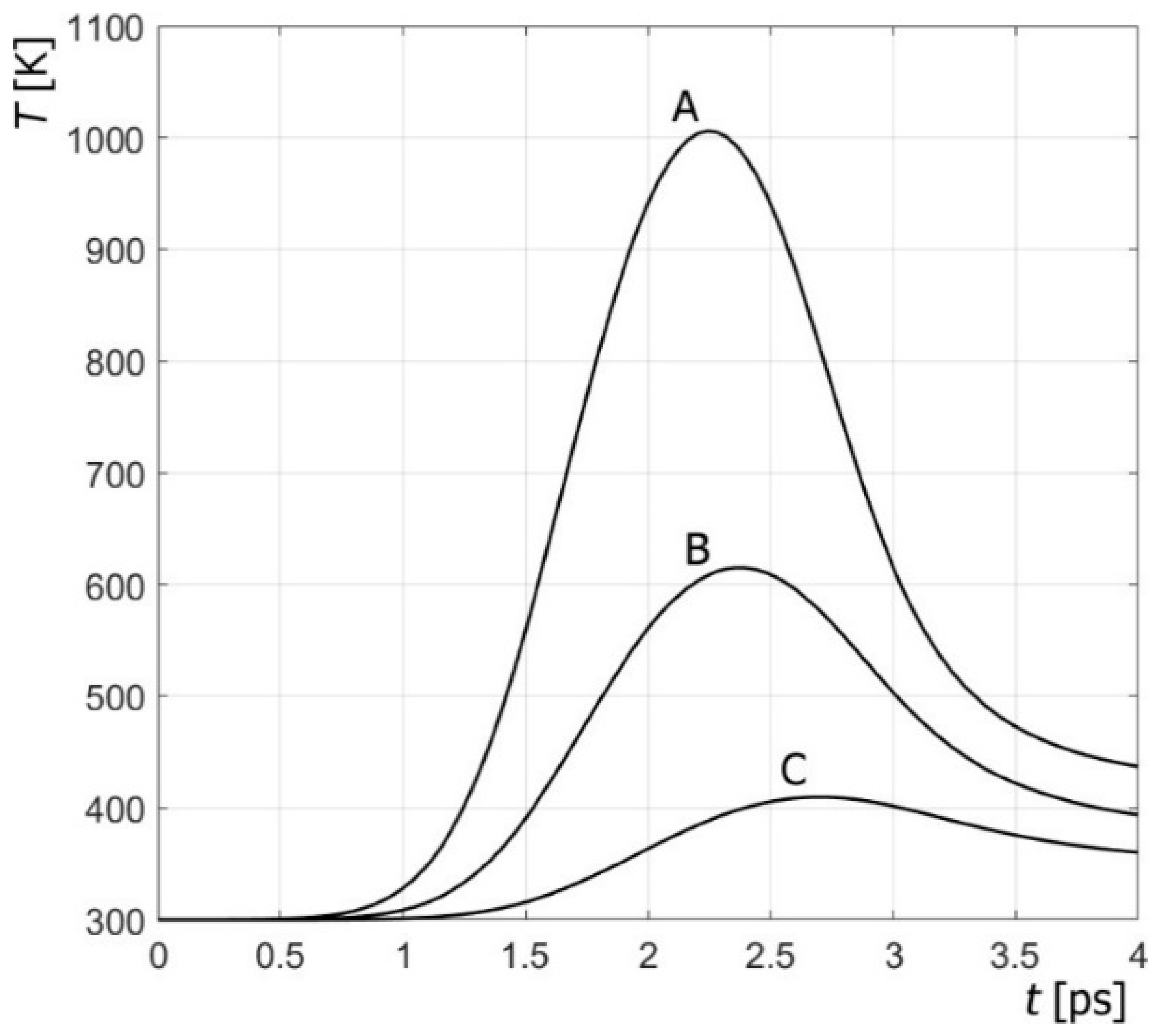
taking into account the variability of thermophysical parameters (especially for higher temperatures) causes visible changes in the results of numerical simulations;
-
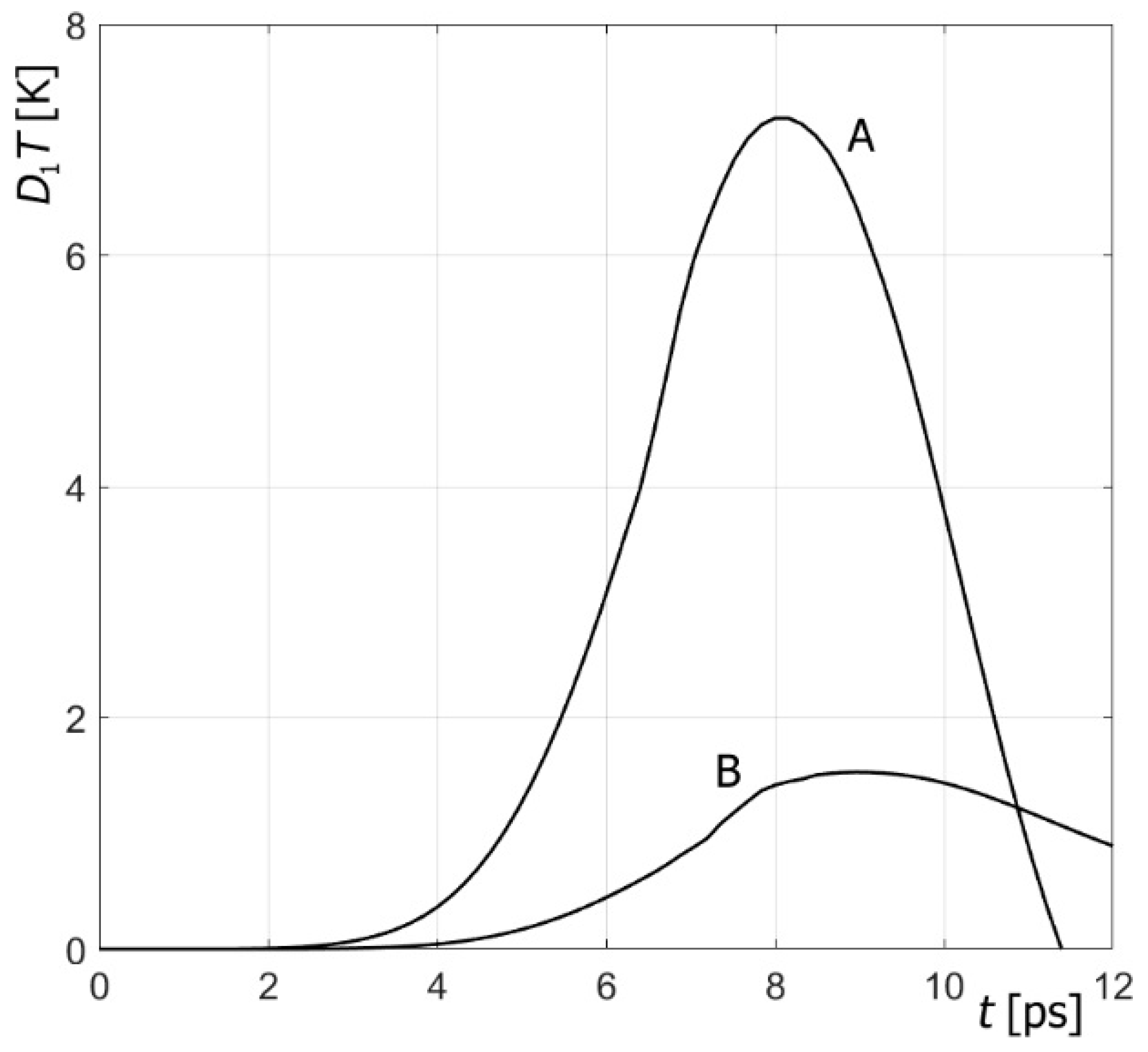
disturbances in the delay-time values clearly change the course of the heating/cooling process in the domain considered;
-
the sensitivity of the temperature field with respect to the delay times increases with the increase in laser intensity;
-
the sensitivity of the temperature field with respect to the delay times varies depending on the type of material and is greater when the metal has a higher mean conductivity coefficient and a lower mean volumetric specific heat.

Author Contributions

Conceptualization, E.M. and B.M.; methodology, B.M.; software, E.M.; formal analysis, E.M. and B.M.; investigation, E.M. and B.M.; resources, E.M.; data curation, B.M.; writing—original draft preparation, B.M.; writing—review and editing, E.M. and B.M.; visualization, E.M.; supervision, E.M.; project administration, E.M.; funding acquisition, E.M. All authors have read and agreed to the published version of the manuscript.

Funding

This research received no external funding.

Data Availability Statement

Data are contained within the article.

Conflicts of Interest

The authors declare no conflicts of interest.

References

  1. Majchrzak, E.; Mochnacki, B. Modelling of thin metal film heating using the dual-phase lag equation with temperature-dependent parameters. Int. J. Heat Mass Transf. 2023, 209, 124088. [Google Scholar] [CrossRef]
  2. Alexopoulou, V.E.; Markopoulos, A.P. A Markopoulos, A critical assessment regarding two-temperature models: An investigation of the different forms of two-temperature models, the various ultrashort pulsed laser models and computational methods. Arch. Comput. Methods Eng. 2023, 31, 93–123. [Google Scholar] [CrossRef]
  3. Majchrzak, E.; Dziatkiewicz, J.; Turchan, L. Analysis of thermal processes occuring in the microdomain subjected to the ultrashort laser pulse using the axisymmetric two-temperature model. Int. J. Multiscale Comput. Eng. 2017, 15, 395–411. [Google Scholar] [CrossRef]
  4. Sobolev, S. Nonlocal two-temperature model: Application to heat transport in metals irradiated by ultrashort laser pulses. Int. J. Heat Mass Transf. 2016, 94, 138–144. [Google Scholar] [CrossRef]
  5. Majchrzak, E.; Mochnacki, B.; Greer, A.; Suchy, J.S. Numerical modeling of short pulse laser interactions with multi-layered thin metal films. CMES Comput. Model. Eng. Sci. 2009, 41, 131–146. [Google Scholar]
  6. Smith, A.N.; Norris, P.M. Microscale Heat Transfer. In Heat Transfer Handbook; John Willey & Sons: Hoboken, NJ, USA, 2003; Chapter 18. [Google Scholar]
  7. Zhang, Z.M. Nano/Microscale Heat Transfer; McGraw-Hill: New York, NY, USA, 2007. [Google Scholar]
  8. Tzou, D.Y. Macro- to Microscale Heat Transfer: The Lagging Behavior; John Wiley & Sons Ltd.: Hoboken, NJ, USA, 2015. [Google Scholar]
  9. Cattaneo, M.C. A form of heat conduction equation which eliminates the paradox of instantaneous propagation. Compte. Rendus. 1958, 247, 431–433. [Google Scholar]
  10. Askarizadeh, H.; Baniasadi, E.; Ahmadikia, H. Equilibrium and non-eqilibrium thermodynamic analysis of high-order dual-phase-lag heat conduction. Int. J. Heat Mass Transf. 2017, 104, 301–309. [Google Scholar] [CrossRef]
  11. Deng, D.; Jiang, Y.; Liang, D. High-order finite difference method for a second order dual-phase-lagging models of microscale heat transfer. Appl. Math. Comput. 2017, 309, 31–48. [Google Scholar] [CrossRef]
  12. Majchrzak, E.; Mochnacki, B. Second-order dual phase-lag equation. Modeling of melting and resolidification of thin metal film subjected to a laser pulse. Mathematics 2020, 8, 999. [Google Scholar] [CrossRef]
  13. Chiriţă, S.; Ciarletta, M.; Tibullo, V. On the thermomechanical consistency of the time differential dual-phase-lag models of heat conduction. Int. J. Heat Mass Transf. 2017, 114, 277–285. [Google Scholar] [CrossRef]
  14. Ciesielski, M.; Mochnacki, B.; Majchrzak, E. Integro-differential form of the first-order dual phase lag heat transfer equation and its numerical solution using the Control Volume Method. Arch. Mech. 2020, 72, 415–444. [Google Scholar]
  15. Xu, H.-Y.; Jiang, X.-Y. Time fractional dual-phase-lag heat conduction equation. Chin. Phys. B 2015, 24, 034401. [Google Scholar] [CrossRef]
  16. Kukla, S.; Siedlecka, U.; Ciesielski, M. Fractional order dual-phase-lag model of heat conduction in a composite spherical medium. Materials 2022, 15, 7251. [Google Scholar] [CrossRef]
  17. Azhdari, M.; Seyedpour, S.M.; Lambers, L.; Tautenhahn, H.-M.; Tautenhahn, F.; Ricken, T.; Rezazadeh, G. Non-local three phase lag bio thermal modeling of skin tissue and experimental evaluation. Int. Commun. Heat Mass Transf. 2023, 149, 107146. [Google Scholar] [CrossRef]
  18. Zhang, Q.; Sun, Y.; Yang, J. Bio-heat response of skin tissue based on three-phase-lag model. Sci. Rep. 2020, 10, 16421. [Google Scholar] [CrossRef]
  19. Chiriţă, S. High-order effects of thermal lagging in deformable conductors. Int. J. Heat Mass Transf. 2018, 127, 965–974. [Google Scholar] [CrossRef]
  20. Quintanilla, R.; Racke, R. A note on stability in dual-phase-lag heat conduction. Int. J. Heat Mass Transf. 2006, 49, 1209–1213. [Google Scholar] [CrossRef]
  21. Arefmanesh, A.; Arani, A.A.A.; Emamifar, A. Semi-analytical solutions for different non-linear models of dual phase lag equation in living tissues. Int. Commun. Heat Mass Transf. 2020, 115, 104596. [Google Scholar] [CrossRef]
  22. Majchrzak, E.; Stryczyński, M. Numerical analysis of biological tissue heating using the dual-phase lag equation with temperature—Dependent parameters. J. Appl. Math. Comput. Mech. 2022, 21, 85–98. [Google Scholar] [CrossRef]
  23. Kumar, R.; Vashishth, A.; Ghangas, S. Phase-lag effects in skin tissue during transient heating. Int. J. Appl. Mech. Eng. 2019, 24, 603–623. [Google Scholar] [CrossRef]
  24. Afrin, N.; Zhou, J.; Zhang, Y.; Tzou, D.Y.; Chen, J.K. Numerical simulation of thermal damage to living biological tissues induced by laser irradiation based on a generalized dual phase lag model. Numer. Heat Transfer Part A Appl. 2012, 61, 483–501. [Google Scholar] [CrossRef]
  25. Shomali, Z.; Kovács, R.; Ván, P.; Kudinov, I.V.; Ghazanfarian, J. Lagging heat models in thermodynamics and bioheat transfer: A critical review. Contin. Mech. Thermodyn. 2022, 34, 637–679. [Google Scholar] [CrossRef]
  26. Ramadan, K. Semi-analytical solutions for the dual phase lag heat conduction in multi-layered media. Int. J. Therm. Sci. 2009, 48, 14–25. [Google Scholar] [CrossRef]
  27. Ciesielski, M. Analytical solution of the dual phase lag equation describing the laser heating of thin metal film. J. Appl. Math. Comput. Mech. 2017, 16, 33–40. [Google Scholar] [CrossRef]
  28. Mohammadi-Fakhar, V.; Momeni-Masuleh, S. An approximate analytic solution of the heat conduction equation at nanoscale. Phys. Lett. A 2010, 374, 595–604. [Google Scholar] [CrossRef]
  29. Ma, J.; Sun, Y.; Yang, J. Analytical solution of dual-phase-lag heat conduction in a finite medium subjected to a moving heat source. Int. J. Therm. Sci. 2018, 125, 34–43. [Google Scholar] [CrossRef]
  30. Kumar, S.; Srivastava, A. Finite integral transform-based analytical solutions of phase lag bio-heat transfer equation. Appl. Math. Model. 2017, 52, 378–403. [Google Scholar] [CrossRef]
  31. Yang, W.; Pourasghar, A.; Cui, Y.; Wang, L.; Chen, Z. Transient heat transfer analysis of a cracked stip irradiated by ultrafast Gaussian laser beam using dual-phase-lag theory. Int. J. Heat Mass Transf. 2023, 203, 123771. [Google Scholar] [CrossRef]
  32. Dutta, J.; Biswas, R.; Kundu, B. Analytical solution of dual-phase-lag based heat transfer model in ultrashort pulse laser heating of A6061 and Cu3Zn2 nano film. Opt. Laser Technol. 2020, 128, 106207. [Google Scholar] [CrossRef]
  33. Wang, H.; Dai, W.; Melnik, R. A finite difference method for studying thermal deformation in a double-layered thin film exposed to ultrashort pulsed lasers. Int. J. Therm. Sci. 2006, 45, 1179–1196. [Google Scholar] [CrossRef]
  34. Chen, J.K.; Beraun, J.E. Numerical study of ultrashort laser pulse interactions with metal films. Numer. Heat Transfer Part A Appl. 2001, 40, 1–20. [Google Scholar] [CrossRef]
  35. Saeed, T.; Abbas, I. Finite element analyses of nonlinear DPL bioheat model in spherical tissues using experimental data. Mech. Based Des. Struct. Mach. 2022, 50, 1287–1297. [Google Scholar] [CrossRef]
  36. Kumar, D.; Rai, K. A study on thermal damage during hyperthermia treatment based on DPL model for multilayer tissues using finite element Legendre wavelet Galerkin approach. J. Therm. Biol. 2016, 62, 170–180. [Google Scholar] [CrossRef] [PubMed]
  37. Majchrzak, E.; Turchan, L. Modeling of laser heating of bi-layered microdomain using the general boundary element method. Eng. Anal. Bound. Elements 2019, 108, 438–446. [Google Scholar] [CrossRef]
  38. Kleiber, M. Parameter Sensitivity in Non-Linear Mechanics; John Willey & Sons Ltd.: London, UK, 1997. [Google Scholar]
  39. Dems, K.; Rousselet, B. Rousselet, Sensitivity analysis for transient heat conduction in a solid body, Part I. Struct. Optim. 1999, 17, 36–45. [Google Scholar] [CrossRef]
  40. Majchrzak, E.; Kałuża, G. Sensitivity analysis of temperature in heated soft tissues with respect to time delays. Contin. Mech. Thermodyn. 2022, 34, 587–599. [Google Scholar] [CrossRef]
  41. Hector, L.G.; Woo-Seung, K.; Özisik, M. Propagation and reflection of thermal waves in a finite medium due to axisymmetric surface sources. Int. J. Heat Mass Transf. 1992, 35, 897–912. [Google Scholar] [CrossRef]
  42. Grigoropoulos, C.P.; Chimmalgi, A.C.; Hwang, D.J. Nano-Structuring Using Pulsed Laser Irradiation, Laser Ablation and Its Applications; Springer Series in Optical Sciences; Springer: Boston, MA, USA, 2007; Volume 129, pp. 473–504. [Google Scholar] [CrossRef]
  43. Huang, J.; Zhang, Y.; Chen, J. Ultrafast solid–liquid–vapor phase change in a thin gold film irradiated by multiple femtosecond laser pulses. Int. J. Heat Mass Transf. 2009, 52, 3091–3100. [Google Scholar] [CrossRef]
  44. Xu, X.; Chen, G.; Song, K. Experimental and numerical investigation of heat transfer and phase change phenomena during excimer laser interaction with nickel. Int. J. Heat Mass Transf. 1999, 42, 1371–1382. [Google Scholar] [CrossRef]
  45. Tang, D.; Araki, N. Wavy, wavelike, diffusive thermal responses of finite rigid slabs to high-speed heating of laser-pulses. Int. J. Heat Mass Transf. 1999, 42, 855–860. [Google Scholar] [CrossRef]
Figure 1. The axially symmetrical domain of the metal.
Energies 17 02252 g001
Figure 2. Temperature distribution after 1.5 ps and 2 ps—gold (I0 = 15,000 W/m2, tp = 1 ps).
Energies 17 02252 g002
Figure 3. Temperature history at points A, B and C—gold (I0 = 15,000 W/m2, tp = 1 ps).
Energies 17 02252 g003
Figure 4. Temperature changes at points A, B and C caused by a perturbation of parameter τq—gold (I0 = 15,000 W/m2, tp = 1 ps).
Energies 17 02252 g004
Figure 5. Temperature changes at points A, B and C caused by a perturbation of parameter τT—gold (I0 = 15,000 W/m2, tp = 1 ps).
Energies 17 02252 g005
Figure 6. Temperature changes at points A, B and C caused by a simultaneous perturbation of parameters τq and τT—gold (I0 = 15,000 W/m2, tp = 1 ps).
Energies 17 02252 g006
Figure 7. Temperature history at points A, B and C—gold (I0 = 10,000 W/m2, tp = 1 ps).
Energies 17 02252 g007
Figure 8. Temperature changes at points A, B and C caused by a perturbation of parameter τq—gold (I0 = 10,000 W/m2, tp = 1 ps).
Energies 17 02252 g008
Figure 9. Temperature changes at points A, B and C caused by a perturbation of parameter τT—gold (I0 = 10,000 W/m2, tp = 1 ps).
Energies 17 02252 g009
Figure 10. Temperature changes at points A, B and C caused by a simultaneous perturbation of parameters τq and τT gold (I0 = 10,000 W/m2, tp = 1 ps).
Energies 17 02252 g010
Figure 11. Temperature distribution after 8 ps and 11 ps—nickel (I0 = 10,000 W/m2, tp = 4 ps).
Energies 17 02252 g011
Figure 12. Temperature history at points A and B—nickel (I0 = 10,000 W/m2, tp = 4 ps).
Energies 17 02252 g012
Figure 13. Temperature changes at points A and B caused by a perturbation of parameter τq—nickel (I0 = 10,000 W/m2, tp = 4 ps).
Energies 17 02252 g013
Figure 14. Temperature changes at points A and B caused by a perturbation of parameter τT—nickel (I0 = 10,000 W/m2, tp = 4 ps).
Energies 17 02252 g014
Figure 15. Temperature changes at points A and B caused by a simultaneous perturbation of parameters τq and τT—nickel (I0 = 10,000 W/m2, tp = 4 ps).
Energies 17 02252 g015
Table 1. Comparison of the results.
Time [ps]0.10.20.30.51.01.52.02.53.0
Experiment0.110.401.00.650.380.240.200.120.10
Model0..110.381.00.670.360.220.190.110.11
Disclaimer/Publisher’s Note: The statements, opinions and data contained in all publications are solely those of the individual author(s) and contributor(s) and not of MDPI and/or the editor(s). MDPI and/or the editor(s) disclaim responsibility for any injury to people or property resulting from any ideas, methods, instructions or products referred to in the content.

