Article

Elevation Accuracy of Forest Road Maps Derived from Aerial Imaging, Airborne Laser Scanning and Mobile Laser Scanning Data

1
Department of Forest Resource Planning and Informatics, Faculty of Forestry, Technical University in Zvolen, T. G. Masaryka 24, 960 01 Zvolen, Slovakia
2
Department of Forest Management, National Forest Centre, T. G. Masaryka 2175/22, 960 01 Zvolen, Slovakia
3
Department of Integrated Geodesy and Cartography, AGH University of Krakow, 30 Mickiewicza Av., 30-059 Krakow, Poland
4
Department of Ecological Engineering and Forest Hydrology, Faculty of Forestry, University of Agriculture in Krakow, 29 Listopada Av. 46, 31-425 Krakow, Poland
5
Department of Forest Harvesting, Logistics and Ameliorations, Faculty of Forestry, Technical University in Zvolen, T. G. Masaryka 24, 960 01 Zvolen, Slovakia
*
Author to whom correspondence should be addressed.
Forests 2024, 15(5), 840; https://doi.org/10.3390/f15050840
Submission received: 20 March 2024 / Revised: 1 May 2024 / Accepted: 7 May 2024 / Published: 10 May 2024
(This article belongs to the Special Issue Recent Advances in Forests Roads Research)

Abstract

:
Forest road maps are a fundamental source of information for the sustainable management, protection, and public utilization of forests. However, the precision of these maps is crucial to their use. In this context, we assessed and compared the elevation accuracy of terrain on three forest road surfaces (i.e., asphalt, concrete, and stone), which were derived based on data from three remote sensing technologies (i.e., aerial imaging, airborne laser scanning, and mobile laser scanning) using five geospatial techniques (i.e., inverse distance; natural neighbor; and conversion by average, maximal, and minimal elevation value). Specifically, the elevation accuracy was assessed based on 700 points at which elevation was measured in the field, and these elevations were extracted from fifteen derived forest road maps with a resolution of 0.5 m. The highest precision was found on asphalt roads derived from mobile laser scanning data (RMSE from ±0.01 m to ±0.04 m) and airborne laser scanning data (RMSE from ±0.03 m to ±0.04 m). On the other hand, the lowest precision was found on all roads derived from aerial imaging data (RMSE from ±0.11 m to ±0.23 m). Furthermore, we found significant differences in elevation between the measured and derived terrains. However, the differences in elevation between specific techniques, such as inverse distance, natural neighbor, and conversion by average, were mostly random. Moreover, we found that airborne and mobile laser scanning technologies provided terrain on concrete and stone roads with random elevation differences. In these cases, it is possible to replace a specific technique or technology with one that is similar without significantly decreasing the elevation accuracy (α = 0.05).

Graphical Abstract

1. Introduction

Forest roads create a logistical network that enables the management, protection, and public utilization of forests [1,2,3,4,5]. For these purposes, relevant stakeholders (e.g., forest owners and managers, policymakers, and the public) need and therefore strictly require forest road maps containing precise information about the related network of forest roads (e.g., location, density, category, and quality) [6,7]. Here, the accuracy of terrain elevation primarily determines the overall precision and, thus, the usability of forest road maps.
Field surveys represent a conventional approach to obtaining information about the terrain on forest roads. Related methods can be considered simple and cheap, but they are sometimes not precise and provide a low rate of points recorded per time unit. For example, steel tape and global navigation satellite systems (GNSSs) are often used to obtain relevant terrain features related to forest roads [8,9].
Remote sensing has recently attracted considerable attention as an alternative approach to improving the efficiency of forest road surveys. Above all, aerial imaging (AI), airborne laser scanning (ALS), and mobile laser scanning (MLS) represent the most innovative remote sensing technologies for acquiring information about the terrain on forest roads [10,11,12,13,14,15].
The application of AI offers several specific photogrammetry methods suitable for creating forest road maps, such as image matching (IM) and structure from motion (SfM). While IM provides data mostly representing the outer canopy [16], SfM offers a more automated workflow, which is more accessible for users and more usable in forest areas [17]. Moreover, SfM enables the generation of two-dimensional as well as three-dimensional terrains using overlapping images acquired from different perspectives with standard compact cameras, including smartphones. It can achieve high performance, especially when used at close range and with dimension stability control (e.g., invar rods) [18]. Thus, SfM represents the most effective AI method applicable to the creation of relatively precise terrains within both non-forest and forest areas [19,20].
ALS is widely used for forest resources and topography mapping since it can provide high-resolution spatial information about forest environments [12,21]. Unlike traditional optical sensors, ALS enables the acquisition of multiple returns, so it is possible to obtain information about forest stands and individual trees, including the understory. Even in areas with dense vegetation, ALS enables the recording of the true ground based on the last returns that penetrate through the gaps of the forest canopy [19,22,23,24]. Thus, the terrain derived from classified ALS point clouds can also reveal road structures in densely forested areas. Various characteristics of forest roads can be derived from ALS data, such as their completeness, road length, positional accuracy, and road grade [12]. Research studies on forest roads have dealt with a wide range of tasks related to these. Some of them are focused on mapping and updating forest road networks [7,25], and others are focused on evaluations of the quality of road surfaces and ditching systems [26]. An approach for forest road extraction and classification using a support vector machine can be applied to classify data into road and non-road classes [27]. Further research has reported applications of ALS data for road detection [13,28,29,30,31], road surface classification [11], forest road damage detection and extraction using deep learning algorithms [32,33], and large-scale road detection in mountainous areas [34].
The application of MLS became popular once it became possible to obtain georeferenced data via real-time GNSS observations. Traditionally, this was performed with total stations and levels, which was a time-consuming technique. Although the dependence of MLS on GNSSs can be considered a drawback because the repeatable accuracy of MLS will be in the same range as a GNSS [35], its advantages surpass the disadvantages. Specifically, MLS systems are multi-discipline combination, multi-sensor integration, and multi-data fusion systems [36] capable of providing accurate and dense point clouds. MLS systems are widely used in urban areas, using various carrying vehicles [37]. Furthermore, they provide fast scanning, can produce very dense point clouds due to the proximity of terrain [10], and can be used as an efficient technology to obtain spatial information about forest roads. They also enable the use of elevation and intensity values for road surface roughness detection [14]. Research on MLS technology applications that focus on forest roads primarily deals with the determination of surface roughness using depth imaging [38], the detection of damage using mobile laser profilometry [37], and the monitoring of wearing courses using cross section analysis [10].
All the remote sensing technologies presented here provide geospatial datasets (coordinates X, Y, and Z of terrain points) that can be used to create terrain on forest roads. However, there is a significant difference in the related elevation accuracy of their final forest road maps. This determines their application, both in practice and in the further processing of associated data as an input for geospatial analyses [39], such as for hydrology [40], forest management [41], and forest transportation [42,43,44]. Here, the quality of the point clouds (e.g., density, horizontal, and vertical accuracy of points) represents a key factor determining the precision of terrain on forest roads [45]. Thus, it is necessary to subordinate the choice of technology to this and know what can be expected from specific sensors with specific settings.
Despite existing research activities being focused on forest transportation, there is a relevant demand for a comprehensive study aimed at comparing the elevation accuracy of forest road maps derived using different geospatial data and techniques (i.e., aerial vs. terrestrial platforms, active vs. passive sensors, and interpolation vs. conversion algorithms).
In this context, the main goal of our study is to assess and compare the elevation accuracy of terrain within forest road maps derived based on data from three remote sensing technologies (i.e., AI, ALS, and MLS) using five geospatial techniques (i.e., inverse distance (IDW); natural neighbor (NN); and conversion by average (PtR-Avg), maximal (PtR-Max), and minimal (PtR-Min) elevation value). Moreover, we conduct this study on three different forest road surfaces (i.e., asphalt, concrete, and stone).

2. Materials and Methods
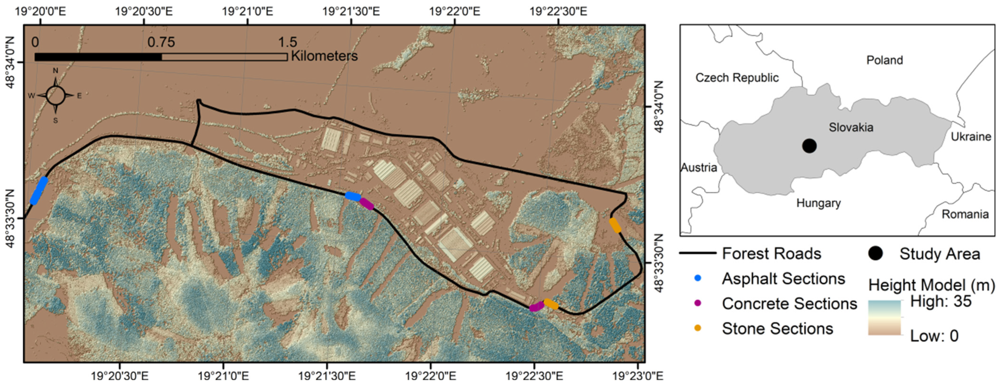
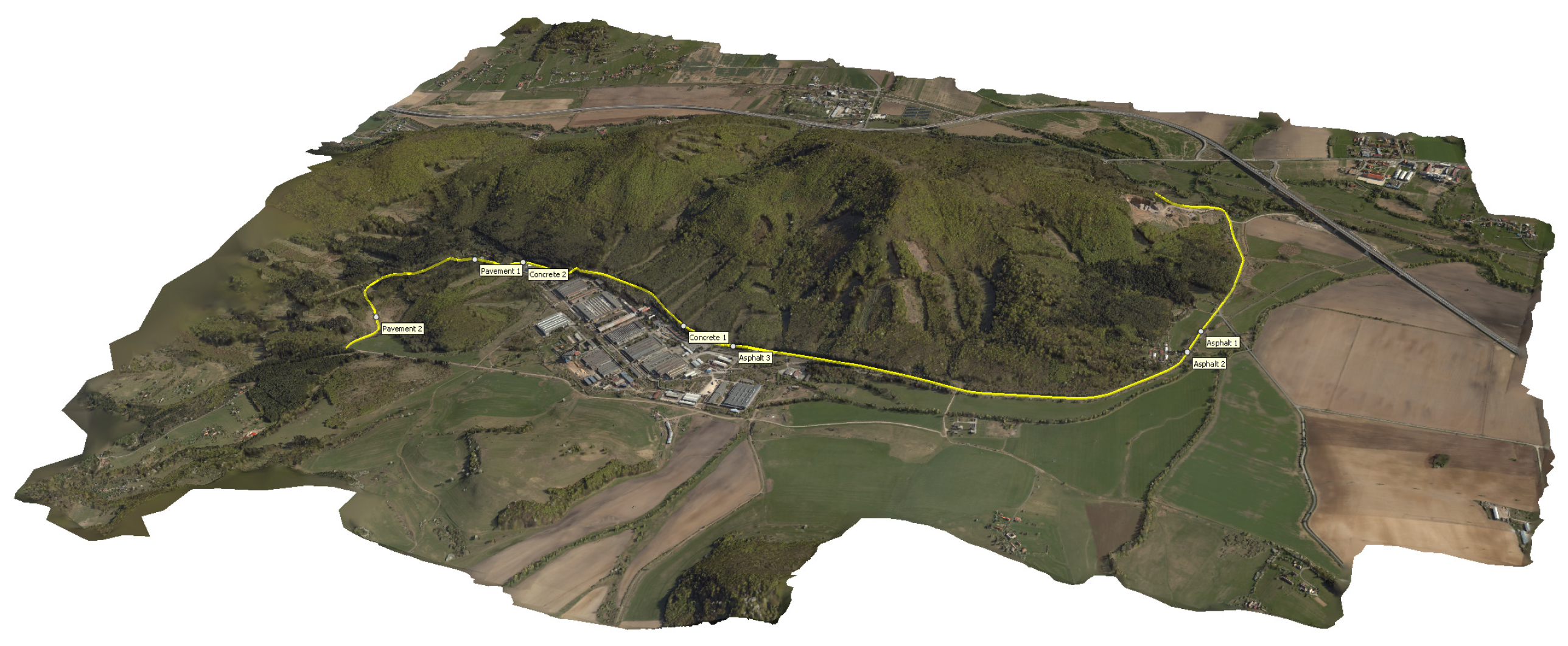
2.1. Study Area

The forest road representing the study area is located in Central Slovakia (Figure 1). The total length of this road is 6238 m, defined by the WGS 84 coordinates of starting point 48.33° N, 19.20° E and ending point 48.34° N, 19.23° E. The elevation range in the Baltic height system is from 359 m to 411 m above sea level.
For the purposes of this study, we selected seven 50 m sections of related forest roads with different surfaces and positions. Specifically, there are three asphalt sections (i.e., 150 m of road with a compact asphalt surface), two concrete sections (i.e., 100 m of road with a partly non-compact surface caused by concrete slabs), and two stone sections (i.e., 100 m of road with an extremely non-compact surface caused by paving stones). The descriptive characteristics of these road surfaces, such as macrostructure derived from intensity values of ALS data and ruggedness calculated from elevation values of terrain, are shown in Figure 2.

2.2. Ground Data

The ground data representing reference dataset were obtained in 2018. We used a geodetic terrestrial measurement approach, combining the GNSS receiver and total station in clear sky conditions to achieve the highest vertical and horizontal accuracy of the reference points. Specifically, a Topcon Hiper GGD and Topcon GPT9003M (Topcon Positioning Systems, Inc., Livermore, CA, USA) were used for these purposes. At least three geodetic points close to each section were measured using GNSS technology to serve as a basis for further detailed measurement with a total station. One of these points served as the position of the total station, and the second and third points served as the orientation and control orientation. We used the single-station method, based on measuring distances and angles to a rod with a prism, for individual reference points. Furthermore, since each section was measured at different times and satellite constellations, we used the GNSS RTK method based on SKPOS corrections (Slovak real-time positioning service). The combination of these methods ensured horizontal and vertical accuracy up to ±0.05 m.
Overall, we measured 700 reference points on the 7 selected sections. Each section included 20 profiles and each profile included 5 reference points. The distance between profiles was ca. 2.5 m and the distance between points was ca. 1.0 m. From this, there were 300 points on the three asphalt surfaces, 200 points on the two concrete surfaces, and 200 points on the two stone surfaces (Figure 3).

2.3. Aerial Imaging Data

The AI data were acquired in 2018 using a Leica RCD 30 camera (Leica Geosystems AG, Heerbrugg, Switzerland) and Cessna 206 aircraft (Cessna AC, Wichita, KS, USA). The survey was conducted in clear sky conditions at an average imaging altitude of 1526 m above ground, with an overlap of 60%/30% and a frame rate of 60 MP/s. The processing of image-based point clouds was performed based on the SfM method using the Agisoft Metashape Professional 2.0.3 software (Agisoft LLC, St. Petersburg, Russia). Here, the orientation was refined using the control points (i.e., individual points on the ground with known coordinates). The classification of ground points was performed based on the Match-T DSM strategy using the INPHO 13 software (Trimble Inc., Westminster, CO, USA). The average density of point clouds within the ground class was 11 points/m2.

2.4. Airborne Laser Scanning Data

The ALS data were acquired in 2018 using a Leica ALS 70 CM scanner (Leica Geosystems AG) and Cessna 206 aircraft (Cessna AC). The survey was conducted in clear sky conditions at an average scanning altitude of 1526 m above ground, with a field of view of 43° and a scan rate of 282 kHz. The processing of ALS-based point clouds was performed using the Leica HxMap software (Hexagon, Stockholm, Sweden). Here, the orientation was refined using control surfaces (i.e., group of points on the surfaces oriented in one height level or slope). The classification of ground points was performed based on the Strong strategy using the INPHO 13 software (Trimble Inc.). The average density of point clouds within the ground class was 9 points/m2.

2.5. Mobile Laser Scanning Data

The MLS data were acquired in 2017 using a Leica Pegasus Two scanner (Leica Geosystems AG) and Ford Ranger 150 truck (Ford MC, Cologne, Germany). The survey was conducted in clear sky conditions at an average scanning altitude of 2 m above ground, with a field of view of 360° × 270° and a scan rate of 1016 kHz. The processing of MLS-based point clouds was performed using the Leica Pegasus Manager software (Hexagon). Here, the orientation was refined using calibrated data from the inertial navigation system (i.e., geospatial dataset from motion and rotation sensors). The classification of ground points was performed based on the Strong strategy using the INPHO 13 software (Trimble Inc.). The average density of point clouds within the ground class was 840 points/m2.

2.6. Generation of Forest Road Maps

The terrain of the forest road maps was generated based on the ground class from the AI, ALS, and MLS point clouds using the ArcGIS Desktop 10.2 software (ESRI, Redlands, CA, USA). Five alternative geospatial terrain generation techniques were used separately for each road surface (i.e., asphalt, concrete, and stone) and data source (i.e., AI, ALS, and MLS). Specifically, terrains were generated using two interpolation techniques and three conversion techniques. The IDW and NN techniques were used for interpolation, and the PtR-Avg, PtR-Max, and PtR-Min techniques were used for conversion. A unified coordinate system (i.e., WGS84/UTM34N) and resolution (i.e., 0.5 m) were used for all data sources and techniques. These data sources were obtained in similar weather and vegetation conditions. In this way, fifteen comparable forest road maps were generated for the purposes of this study.

2.7. Assessment of Elevation Accuracy of Forest Road Maps

The elevation accuracy of the forest road maps was assessed by comparing the measured terrain (i.e., reference dataset) and generated terrain (i.e., derived dataset). Specifically, we used seven hundred points (n) where elevations were measured using a combination of a GNSS and total station (zMT) and where elevations were extracted from all fifteen types of generated terrains (zGT). A comparison of paired elevations was performed based on an error matrix consisting of key accuracy attributes, such as individual difference, ei (Equation (1)); mean difference, ē (Equation (2)); standard deviation of mean difference, se (Equation (3)); and total difference in terms of root mean square error, RMSE (Equation (4)) (i.e., 68% confidence interval). Additionally, the p-value of the normality test (i.e., Shapiro–Wilk W test) and paired test (i.e., Student’s or Wilcoxon’s pair test) was calculated to evaluate the related significance of differences at the α = 0.05 significance level and at f = n − 1 degrees of freedom (i.e., 95% confidence interval).
e i = z G T i z M T i
e ¯ = i = 1 n e i n
s e = i = 1 n ( e i e ¯ ) 2 n 1
R M S E = s e 2 + e ¯ 2

3. Results

The three-dimensional visualization of the final forest road map with a resolution of 0.5 m is displayed in Figure 4. While MLS provided relatively high detail for all road surfaces, ALS only offered this level of detail for the roads with a stone surface. The visibility and level of detail of the forest roads derived from AI data were relatively low or non-existent (Figure 5).
The elevation accuracy values of the forest road maps (i.e., asphalt, concrete, and stone roads) derived from AI, ALS, and MLS data using five geospatial techniques (i.e., IDW, NN, PtR-Avg, PtR-Max, and PtR-Min) are reported in Table 1.
The mean elevation difference was in the range of −0.02 m to 0.20 m (asphalt roads), −0.04 m to 0.10 m (concrete roads), and −0.05 m to 0.05 m (stone roads), depending on the technique. Negative values (i.e., underestimations) were found primarily on concrete roads derived from ALS and MLS data. Here, the PtR-Min technique also provided negative values on other forest roads. However, none of these elevation differences exceeded the value of −0.05 m. Positive elevation differences (i.e., overestimations) were found with all other forest roads and techniques. In particular, the application of AI data resulted in the highest positive elevation differences with the largest variability on all forest road surfaces (0.01 m to 0.20 m).
The total elevation difference was in the range of ±0.01 m to ±0.23 m (asphalt roads), ±0.02 m to ±0.19 m (concrete roads), and ±0.03 m to ±0.13 m (stone roads), depending on the technique. The lowest values (i.e., highest elevation accuracy) were found on asphalt roads derived from MLS data (±0.01 m to ±0.04 m). Other forest roads derived from ALS and MLS data achieved a range of ±0.02 m to ±0.07 m. The highest values (i.e., the lowest elevation accuracy) were found on all forest roads derived from AI data (±0.11 m to ±0.23 m). In particular, the application of AI data on asphalt roads provided the highest elevation differences, in the range of ±0.20 m to ±0.23 m.
The significance of the elevation differences in the forest road maps (i.e., asphalt, concrete, and stone roads) derived from AI, ALS, and MLS data using five geospatial techniques (i.e., IDW, NN, PtR-Avg, PtR-Max, and PtR-Min) is reported in Table 2, Table 3, Table 4 and Table 5 (α = 0.05).
The elevations of the concrete and stone roads derived from AI data and the asphalt roads derived from ALS data using the PtR-Min technique were not statistically significant relative to the elevations in the ground data. Here, the stone roads derived from AI data using the IDW, NN, and PtR-Avg techniques and the concrete roads derived from MLS data using the PtR-Max technique were not statistically significant either. Other road surfaces, data sources, and techniques significantly affected the elevation accuracy of the forest road maps (i.e., differences between the derived and real terrain).
The elevation differences between the forest road maps derived using the IDW, NN, and PtR-Avg techniques were mostly not significant regardless of the road surface (i.e., difference between techniques).
The elevation differences between ALS-based and MLS-based concrete roads derived using the IDW, NN, and PtR-Avg techniques and stone roads derived using the PtR-Min technique were not statistically significant. In other cases, different data sources provided forest road maps with significantly different elevations (i.e., differences between technologies).

4. Discussion

Our study assessed and compared the elevation accuracy of terrain within forest road maps derived from data obtained with three remote sensing technologies (i.e., AI, ALS, and MLS) using five geospatial techniques (i.e., IDW, NN, PtR-Avg, PtR-Max, and PtR-Min). Moreover, we conducted this comparison on three different forest road surfaces (i.e., asphalt, concrete, and stone).
The application of MLS data and the IDW, NN, and PtR-Avg techniques provided the best results in our study when considering the elevation accuracy, point cloud density, and quality of the final forest road maps. In these cases, the RMSE did not exceed the interval of ±0.03 m. Thus, the precision of the MLS-based forest map was within the theoretical limit of accuracy for this remote sensing technology (i.e., ±0.03 m [35]). Moreover, the terrain of forest roads included the finest details that enabled further geospatial analysis, such as damage detection and the assessment of related costs for reconstruction. Most of the other associated studies confirm our results. For example, Hoffmann and Brenner (2016) [46] analyzed the elevation accuracy of MLS point clouds obtained with a RIEGL VMX-250 system. They achieved a difference of 0.08 m before the adjustments and up to 0.01 m with adjusted data. The elevation accuracy of the MLS point clouds obtained with a LARA 3D system was evaluated within the study of Poreba and Goulette (2012) [47]. Similar to our study, accuracy was assessed using a reference dataset measured by a total station and a difference of up to 0.30 m was achieved. On the other hand, Hruza et al. (2018) [10] provided opposite results to those of our study. They also used AI, ALS, and MLS data to compare the elevation accuracy of forest roads. However, MLS data obtained with a RIEGL VMX-450 achieved the highest elevation difference (i.e., the lowest precision). The lower accuracy here, reflected in a total difference of ±0.32 m and a mean difference of −0.66 m, was probably caused by the lack of an absolute orientation of the MLS system under the forest canopy.
The ALS data provided forest road maps with a slightly worse elevation accuracy than the MLS data in our study. However, their accuracy was still much higher than that obtained with the application of AI data. Specifically, the RMSE of ALS-based forest maps did not exceed the interval of ±0.06 m. Thus, ALS data also met the theoretical limit of accuracy for this remote sensing technology (i.e., ±0.20 m; e.g., [48]). On the other hand, there was clearly less detail for the road surfaces than in the case of MLS-based forest roads. Other studies have provided similar results. Sačkov and Kardoš (2014) [49] analyzed the elevation accuracy of ALS-based terrain derived from point clouds with a density ranging from 1.7 points/m2 to 2.5 points/m2. The RMSE ranged from ±0.13 m to ±0.18 m, depending on the density of the forest canopy (i.e., leaf-off or leaf-on conditions). Hyyppä et al. (2004) [50] reported random elevation differences of less than 0.20 m in non-steep terrain. They used ALS point clouds with densities of 8–10, 4–5, and 2–3 points/m2. Balenović et al. (2018) [51] analyzed the elevation accuracy of ALS-based terrain in a lowland oak forest. The RMSE values ranged from ±0.14 m to ±0.15 m while the elevation differences decreased with decreasing spatial resolution of the terrain.
In our study, the elevation accuracy of the forest road maps obtained using AI data was the lowest, compared to the application of ALS or MLS data, despite the fact that AI data provided relatively dense point clouds (i.e., 11 points/m2). Specifically, the RMSE of AI-based forest maps achieved an interval from ±0.11 m to ±0.23 m. Here, the theoretical limit of accuracy was 0.23 m, based on the equations of Kraus (2004) [52] and Karel et al. (2006) [53]. Although this theoretical limit was not exceeded, AI remains the most challenging among the tested remote sensing technologies (i.e., ALS and MLS). Some factors that affect the related precision are the flying height, focal length, spatial resolution, and the environment of the area, where the surrounding forest stands and their shadows have the most significant effect on the degradation of elevation accuracy. Here, the objects (e.g., trees and their shadows) can cover the surface of the forest road to different degrees depending on the camera’s position at the time of exposure. Due to these obstacles, this data source should be reduced to contain only points on the forest road surface in order to perform the analysis correctly. Moreover, relief displacements occur radially as the distance from the principal point of the image increases [54], meaning that the objects on the terrain tend to tilt as the distance increases. From this point of view, AI seems to be the least suitable data source for generating precise forest road terrain under or near forest stands. Furthermore, the elevation accuracies achieved in this study correspond with the capabilities of image correlation, which, by identifying pairs of points and the horizontal parallaxes between them, calculates heights for points with a point density depending on the pixel size. Traditionally, image correlation provides better results on surfaces with a heterogeneous texture, which, in our case, was the stone surface. Considering this fact, we assume that the homogenous surface texture was the leading cause of the lower elevation accuracy on asphalt roads. Our practical experience with image matching for terrain generation based on AI data is also supported by the conclusions of Rahmayudi and Rizaldy (2016) [55]. They concluded that many factors influence terrain generation using a semiautomatic image-matching method. Here, homogeneous areas were the leading cause of error points in mountainous and flat terrain. AI-based terrain in such areas tends to be lower than the real values and depression points emerge. Finally, several other factors influenced the precision of AI-based terrains, such as the type of lens used, in this case one with a 53 mm focal length; the flying height; the GSD resolution; and the overlap of the images. Based on these facts, it can be concluded that AI data obtained at a lower flight height and during the leaf-off season should be used in order to provide precise forest road maps. The optimum solution appears to be remotely piloted aircraft systems, which enable images to be obtained at a height of a few meters from the road surface. These facts are also confirmed by studies that have utilized AI data from different environmental conditions and technology platforms. For example, Balenović et al. (2018) [51] provided AI-based terrains under a forest canopy with an RMSE of ±0.35 m, regardless of terrain resolution. Botes [35] conducted research outside of a forest environment and achieved similar results to our study. They achieved an RMSE value of ±0.14 m. Finally, Hobi et al. (2012) [56] derived terrain from satellite multi-spectral images (i.e., WorldView-2) and achieved an RMSE of ±0.32 m.
In view of the above outcomes, the precision of the ALS-based, MLS-based, and even AI-based forest road maps was within the theoretical limit of elevation accuracy for the related remote sensing technology. However, associated differences between derived and real elevations were mostly significant. This was detected using the Student’s or Wilcoxon’s paired statistical tests at the α = 0.05 significance level. The only exceptions (i.e., random differences between derived and real terrain) to this were asphalt roads derived from ALS data using the PtR-Min technique, concrete roads derived from AI data using the PtR-Min technique and from MLS data using the PtR-Max technique, and stone roads derived from AI data using the IDW, NN, PtR-Avg, and PtR-Min techniques. Similarly, the IDW, NN, and PtR-Avg techniques mostly provided forest road maps with random elevation differences (i.e., random difference between techniques). Finally, these random elevation differences were also found between specific data sources. The elevation differences between ALS-based and MLS-based concrete roads derived using the IDW, NN, and PtR-Avg techniques, and stone roads derived using the PtR-Min technique were not significant (i.e., random differences between technologies). In all these cases, an alternative remote sensing technology or geospatial technique could be used within a 95% confidence interval without significant changes in the elevation accuracy. Since these findings are in line with other studies, e.g., [23,57,58,59,60], it can be stated that in specific cases it is possible to replace MLS technology with the less economically demanding ALS technology. This is particularly feasible if there is no need for forest road maps with a high level of detail.

5. Conclusions

Remote sensing technologies have proven to be a reliable source of geospatial data for forest road mapping. Here, the elevation accuracy of terrain primarily determines the overall precision and, thus, the usability of the related maps. In this context, we assessed and compared the elevation accuracy of terrain on asphalt, concrete, and stone roads derived from data obtained with three remote sensing technologies (i.e., AI, ALS, and MLS) using five geospatial techniques (i.e., IDW, NN, PtR-Avg, PtR-Max, and PtR-Min).
The AI-based forest road maps achieved elevation accuracies from ±0.17 m to ±0.20 m in terms of RMSE. The best results were provided by the PtR-Min technique. The visibility and level of detail of terrain on forest roads were relatively low or non-existent. Moreover, this terrain contained large errors at the edges of roads that were close to the forest stands. For these reasons, we recommend only using this technology in open areas or when taking images during the off-growing (i.e., leaf-off) season. For this purpose, it would be advisable to use a higher image overlap (e.g., 80 × 60%) and lenses with a longer focal length to avoid significant radial distortion in the images.
The ALS-based forest road maps achieved an elevation accuracy of ±0.05 m in terms of RMSE. There were minimal differences between techniques. A high visibility and level of detail of the terrain on forest roads were only obtained for roads with a stone surface. The elevation differences between the ALS-based and MLS-based concrete and stone roads were not significant. Thus, it is possible to replace MLS with the less economically demanding ALS technology in these cases if there is no need for a high level of detail.
The MLS-based forest road maps achieved elevation accuracies from ±0.02 m to ±0.05 m in terms of RMSE. The IDW, NN, and PtR-Avg techniques provided the best results. This technology provided forest road maps with the highest elevation accuracy, visibility, and level of detail for all road surfaces. However, from a practical point of view and in terms of this study, MLS technology provides only limited auxiliary information and is mainly limited to single-purpose applications (e.g., forest road mapping). Therefore, stakeholders must choose to either receive complex information about the environment with lower accuracy (e.g., aerial or satellite data sources) or obtain highly accurate data with limited broader context (e.g., terrestrial data sources).
These results provide a useful source of information for relevant stakeholders related to the management, protection, and utilization of forests. However, related research was focused only on the highest category of forest roads located outside the forest (i.e., fully paved haul forest roads with a uniform surface and a longitudinal slope of up to 10%). Future studies should, therefore, include samples of geospatial data from different environments to assess the impact of varying weather conditions, terrain roughness, and vegetation cover on the elevation accuracy of forest road maps.

Author Contributions

Conceptualization, methodology, resources: M.K. and I.S.; validation and formal analysis: J.T., Ł.B., M.F. and I.B.; writing—original draft preparation: M.K. and I.S.; writing—review and editing: I.S.; funding acquisition: M.K., J.T. and Ł.B. All authors have read and agreed to the published version of the manuscript.

Funding

This research was funded by the project FOMON-ITMS 313011V465, supported by the Operational Program Integrated Infrastructure (OPII) funded by the ERDF (80%), and the project VEGA MŠ SR and SAV 1/0568/23, the application of Global Navigation Satellite Systems (GNSSs) signals for localization and monitoring of vegetation in the forest environment (20%).

Data Availability Statement

The data presented in this study are available on request from the corresponding author.

Conflicts of Interest

The authors declare no conflicts of interest.

References

  1. Hunt, L.M.; Hosegood, S. The Effectiveness of Signs at Restricting Vehicle Traffic: A Case of Seasonal Closures on Forest Access Roads. Can. J. For. Res. 2008, 38, 2306–2312. [Google Scholar] [CrossRef]
  2. Dudáková, Z.; Ferenčík, M.; Allman, M.; Merganičová, K.; Merganič, J.; Vlčková, M. Who Uses Forest Roads? Has the COVID-19 Pandemics Affected Their Recreational Usage? Case Study from Central Slovakia. Forests 2022, 13, 458. [Google Scholar] [CrossRef]
  3. Apollo, M.; Andreychouk, V. Trampling Intensity and Vegetation Response and Recovery According to Altitude: An Experimental Study from the Himalayan Miyar Valley. Resources 2020, 9, 98. [Google Scholar] [CrossRef]
  4. Apollo, M.; Andreychouk, V.; Bhattarai, S.S. Short-Term Impacts of Livestock Grazing on Vegetation and Track Formation in a High Mountain Environment: A Case Study from the Himalayan Miyar Valley (India). Sustainability 2018, 10, 951. [Google Scholar] [CrossRef]
  5. Fidelus-Orzechowska, J.; Strzyżowski, D.; Żelazny, M. The Geomorphic Activity of Forest Roads and Its Dependencies in the Tatra Mountains. Geogr. Ann. Ser. A Phys. Geogr. 2018, 100, 59–74. [Google Scholar] [CrossRef]
  6. Lehtomäki, M.; Jaakkola, A.; Hyyppä, J.; Kukko, A.; Kaartinen, H. Detection of Vertical Pole-Like Objects in a Road Environment Using Vehicle-Based Laser Scanning Data. Remote Sens. 2010, 2, 641–664. [Google Scholar] [CrossRef]
  7. Morley, I.; Coops, N.; Roussel, J.-R.; Achim, A.; Dech, J.; Meecham, D.; McCartney, G.; Reid, D.; McPherson, S.; Quist, L.; et al. Updating Forest Road Networks Using Single Photon LiDAR in Northern Forest Environments. For. Int. J. For. Res. 2023, 97, 38–47. [Google Scholar] [CrossRef]
  8. Labelle, E.R.; Poltorak, B.; Jaeger, D. Soil Displacement during Ground-Based Mechanized Forest Operations Using Mixed-Wood Brush Mats. Soil Tillage Res. 2018, 179, 96–104. [Google Scholar] [CrossRef]
  9. Cambi, M.; Certini, G.; Fabiano, F.; Foderi, C.; Laschi, A.; Picchio, R. Impact of Wheeled and Tracked Tractors on Soil Physical Properties in a Mixed Conifer Stand. Iforest Biogeosciences For. 2015, 9, e1–e6. [Google Scholar] [CrossRef]
  10. Hrůza, P.; Mikita, T.; Tyagur, N.; Krejza, Z.; Cibulka, M.; Procházková, A.; Patočka, Z. Detecting Forest Road Wearing Course Damage Using Different Methods of Remote Sensing. Remote Sens. 2018, 10, 492. [Google Scholar] [CrossRef]
  11. Karila, K.; Matikainen, L.; Puttonen, E.; Hyyppä, J. Feasibility of Multispectral Airborne Laser Scanning Data for Road Mapping. IEEE Geosci. Remote Sens. Lett. 2017, 14, 294–298. [Google Scholar] [CrossRef]
  12. White, R.A.; Dietterick, B.C.; Mastin, T.; Strohman, R. Forest Roads Mapped Using LiDAR in Steep Forested Terrain. Remote Sens. 2010, 2, 1120–1141. [Google Scholar] [CrossRef]
  13. Buján, S.; Guerra, J.; González-Ferreiro, E.; Miranda, D. Forest Road Detection Using LiDAR Data and Hybrid Classification. Remote Sens. 2021, 13, 393. [Google Scholar] [CrossRef]
  14. Kumar, P.; Angelats, E. An Automated Road Roughness Detection from Mobile Laser Scanning Data. ISPRS Int. Arch. Photogramm. Remote Sens. Spat. Inf. Sci. 2017; XLII-1/W1, 91–96. [Google Scholar] [CrossRef]
  15. Mikita, T.; Krausková, D.; Hrůza, P.; Cibulka, M.; Patocka, Z. Forest Road Wearing Course Damage Assessment Possibilities with Different Types of Laser Scanning Methods Including New iPhone LiDAR Scanning Apps. Forests 2022, 13, 1763. [Google Scholar] [CrossRef]
  16. Goodbody, T.R.H.; Coops, N.C.; White, J.C. Digital Aerial Photogrammetry for Updating Area-Based Forest Inventories: A Review of Opportunities, Challenges, and Future Directions. Curr For. Rep 2019, 5, 55–75. [Google Scholar] [CrossRef]
  17. Fonstad, M.A.; Dietrich, J.T.; Courville, B.C.; Jensen, J.L.; Carbonneau, P.E. Topographic Structure from Motion: A New Development in Photogrammetric Measurement. Earth Surf. Process. Landf. 2013, 38, 421–430. [Google Scholar] [CrossRef]
  18. Borowski, Ł.; Pieńko, M.; Wielgos, P. Evaluation of Inventory Surveying of Façade Scaffolding Conducted during ORKWIZ Project. In Proceedings of the 2017 Baltic Geodetic Congress (BGC Geomatics), Gdansk, Poland, 22–25 June 2017; pp. 189–192. [Google Scholar] [CrossRef]
  19. Gil, A.L.; Núñez-Casillas, L.; Isenburg, M.; Benito, A.A.; Bello, J.J.R.; Arbelo, M. A Comparison between LiDAR and Photogrammetry Digital Terrain Models in a Forest Area on Tenerife Island. Can. J. Remote Sens. 2013, 39, 396–409. [Google Scholar] [CrossRef]
  20. Iglesias, L.; De Santos-Berbel, C.; Pascual, V.; Castro, M. Using Small Unmanned Aerial Vehicle in 3D Modeling of Highways with Tree-Covered Roadsides to Estimate Sight Distance. Remote Sens. 2019, 11, 2625. [Google Scholar] [CrossRef]
  21. Apollo, M.; Jakubiak, M.; Nistor, S.; Lewińska, P.; Krawczyk, A.; Borowski, Ł.; Specht, M.; Krzykowska-Piotrowska, K.; Marchel, Ł.; Pęska-Siwik, A.; et al. Geodata in Science—A Review of Selected Scientific Fields. Acta Sci. Pol. Form. Circumiectus 2023, 22, 17–40. [Google Scholar] [CrossRef]
  22. Maciuk, K.; Apollo, M.; Mostowska, J.; Lepeška, T.; Poklar, M.; Noszczyk, T.; Kroh, P.; Krawczyk, A.; Borowski, Ł.; Pavlovčič-Prešeren, P. Altitude on Cartographic Materials and Its Correction According to New Measurement Techniques. Remote Sens. 2021, 13, 444. [Google Scholar] [CrossRef]
  23. Reutebuch, S.E.; McGaughey, R.J.; Andersen, H.-E.; Carson, W.W. Accuracy of a High-Resolution Lidar Terrain Model under a Conifer Forest Canopy. Can. J. Remote Sens. 2003, 29, 527–535. [Google Scholar] [CrossRef]
  24. Kraus, K.; Pfeifer, N. Determination of Terrain Models in Wooded Areas with Airborne Laser Scanner Data. ISPRS J. Photogramm. Remote Sens. 1998, 53, 193–203. [Google Scholar] [CrossRef]
  25. David, N.; Mallet, C.; Pons, T.; Chauve, A.; Bretar, F. Pathway Detection and Geometrical Description from ALS Data in Forested Moutaneous Area. In Laser Scanning; Bretar, F., Pierrot-Deseilligny, M., Vosselman, G., Eds.; IAPRS: Paris, France, 2009; Volume 38, pp. 242–247. [Google Scholar]
  26. Waga, K.; Malinen, J.; Tokola, T. Forest Road Quality Control Using ALS Data. Can. J. For. Res. 2015, 45, 11. [Google Scholar] [CrossRef]
  27. Azizi, Z.; Najafi, A.; Sadeghian, S. Forest Road Detection Using LiDAR Data. J. For. Res. 2014, 25, 975–980. [Google Scholar] [CrossRef]
  28. Clode, S.; Rottensteiner, F.; Kootsookos, P.; Zelniker, E. Detection and Vectorization of Roads from Lidar Data. Photogramm. Eng. Remote Sens. 2007, 73, 517–535. [Google Scholar] [CrossRef]
  29. Hejmanowska, B.; Warchoł, A. Comparison of the Elevation Obtained from Als, Ads40 Stereoscopic Measurements and GPS. Acta Sci. Pol. Geod. Et Descr. Terrarum 2010, 9, 13–24. [Google Scholar]
  30. Warchoł, A. Use of Signal Intensity Indices in The Process of Extracting A Road Network From Lidar Data. Arch. Fotogram. Kartogr. I Teledetekcji 2009, 20, 433–444. [Google Scholar]
  31. Prendes Pérez, C.; Buján, S.; Ordóñez, C.; Canga, E. Large Scale Semi-Automatic Detection of Forest Roads from Low Density LiDAR Data on Steep Terrain in Northern Spain. Iforest Biogeosciences For. 2019, 12, 366–374. [Google Scholar] [CrossRef]
  32. Heidari, M.; Najafi, A.; Borges, J. Forest Roads Damage Detection Based on Deep Learning Algorithms. Scand. J. For. Res. 2022, 37, 366–375. [Google Scholar] [CrossRef]
  33. Kearney, S.P.; Coops, N.; Sethi, S.; Stenhouse, G. Maintaining Accurate, Current, Rural Road Network Data: An Extraction and Updating Routine Using RapidEye, Participatory GIS and Deep Learning. Int. J. Appl. Earth Obs. Geoinf. 2020, 87, 102031. [Google Scholar] [CrossRef]
  34. Ferraz, A.; Mallet, C.; Chehata, N. Large-Scale Road Detection in Forested Mountainous Areas Using Airborne Topographic Lidar Data. ISPRS J. Photogramm. Remote Sens. 2016, 112, 23–36. [Google Scholar] [CrossRef]
  35. Botes, D. Accuracy Assessment: Mobile Laser Scanning versus Competing Methods. In Proceedings of the South African Surveying and Geomatics Indaba (SASGI) Proceedings, Ekurhuleni, South Africa, 23–24 July 2013; p. 16. [Google Scholar]
  36. Xu, S.; Cheng, P.; Zhang, Y.; Ding, P. Error Analysis and Accuracy Assessment of Mobile Laser Scanning System. Open Autom. Control. Syst. J. 2015, 7, 485–495. [Google Scholar] [CrossRef]
  37. Ferenčík, M.; Kardoš, M.; Allman, M.; Slatkovská, Z. Detection of Forest Road Damage Using Mobile Laser Profilometry. Comput. Electron. Agric. 2019, 166, 105010. [Google Scholar] [CrossRef]
  38. Marinello, F.; Proto, A.R.; Zimbalatti, G.; Pezzuolo, A.; Cavalli, R.; Grigolato, S. Determination of Forest Road Surface Roughness by Kinect Depth Imaging. Ann. For. Res. 2017, 60, 2. [Google Scholar] [CrossRef]
  39. Burrough, P.A. Principles of Geographical Information Systems for Land Resources Assessment; Oxford [Oxfordshire]; Clarendon Press: New York, NY, USA; Oxford University Press: Oxford, UK, 1986; ISBN 978-0-19-854563-7. [Google Scholar]
  40. Jaara, K.; Lecordix, F. Extraction of Cartographic Contour Lines Using Digital Terrain Model (DTM). Cartogr. J. 2011, 48, 131–137. [Google Scholar] [CrossRef]
  41. Wulder, M.; Bater, C.; Coops, N.; Hilker, T.; White, J. The Role of LiDAR in Sustainable Forest Management. For. Chron. 2008, 84, 807–826. [Google Scholar] [CrossRef]
  42. Aruga, K.; Sessions, J.; Miyata, E.S. Forest Road Design with Soil Sediment Evaluation Using a High-Resolution DEM. J Res 2005, 10, 471–479. [Google Scholar] [CrossRef]
  43. Taş, İ.; KASKA, M.; Akay, A. Assessment of Using UAV Photogrammetry Based DEM and Ground-Measurement Based DEM in Computer-Assisted Forest Road Design. Eur. J. For. Eng. 2023, 9, 1–9. [Google Scholar] [CrossRef]
  44. Danilović, M.; Ristić, R.; Stojnić, D.; Antonić, S.; Dražić, S. Evaluation of Morphometric Terrain Parameters and Their Influence on Determining Optimal Density of Primary Forest Road Network. Croat. J. For. Eng. 2023, 44, 12. [Google Scholar] [CrossRef]
  45. Skaloud, J.; Schaer, P. Automated Assessment of Digital Terrain Models Derived From Airborne Laser Scanning. Photogramm. Fernerkund. Geoinf. 2012, 2012, 105–114. [Google Scholar] [CrossRef]
  46. Hofmann, S.; Brenner, C. Accuracy Assessment of Mobile Mapping Point Clouds Using the Existing Environment as Terrestrial Reference. ISPRS Int. Arch. Photogramm. Remote Sens. Spat. Inf. Sci. 2016; XLI-B1, 601–608. [Google Scholar] [CrossRef]
  47. Poreba, M.; Goulette, F. Assesing the Accuracy of Terrestrial Mobile Laser Surveys. Geomat. Enironmental Eng. 2012, 6, 73–81. [Google Scholar] [CrossRef]
  48. Höhle, J.; Potuckova, M.; Assessment of the Quality of Digital Terrain Models. Official Publication–EuroSDR 2011. Available online: http://www.eurosdr.net/sites/default/files/uploaded_files/eurosdr_publication_ndeg_60.pdf (accessed on 19 March 2024).
  49. Sačkov, I.; Kardoš, M. Forest Delineation Based on LiDAR Data and Vertical Accuracy of the Terrain Model in Forest and Non-Forest Area. Ann. For. Res. 2014, 57, 1. [Google Scholar] [CrossRef]
  50. Hyyppä, H.; Yu, X.; Hyyppä, J.; Kaartinen, H.; Kaasalainen, S.; Honkavaara, E.; Rönnholm, P. Factors Affecting the Quality of DTM Generation in Forested Areas. Int. Arch. Photogramm. Remote Sens. Spat. Inf. Sci 2004, 36, 85–90. [Google Scholar]
  51. Balenović, I.; Gasparovic, M.; Anita, S.M.; Berta, A.; Seletković, A. Accuracy Assessment of Digital Terrain Models of Lowland Pedunculate Oak Forests Derived from Airborne Laser Scanning and Photogrammetry. Croat. J. For. Eng. 2018, 39, 117–128. [Google Scholar]
  52. Kraus, K. Photogrammetrie; Walter de Gruyter: Berlin, Germany, 2004; ISBN 978-3-11-017708-4. [Google Scholar]
  53. Karel, W.; Pfeifer, N.; Briese, C. Dtm quality assessment. In Proceedings of the ISPRS Technical Commission II Symposium, Vienna, Austria, 12–14 July 2006; p. 6. [Google Scholar]
  54. Wolf, R.P.; Dewitt, A.B.; Wilkinson, E.B. Elements of Photogrammetry with Applications in GIS, 4th ed.; McGraw-Hill Education, New York, NY, USA, 2014; ISBN 978-0-07-176112-3.
  55. Rahmayudi, A.; Rizaldy, A. Comparison of Semi Automatic DTM from Image Matching with DTM from Lidar. ISPRS Int. Arch. Photogramm. Remote Sens. Spat. Inf. Sci. 2016; XLI-B3, 373–380. [Google Scholar] [CrossRef]
  56. Hobi, M.L.; Ginzler, C. Accuracy Assessment of Digital Surface Models Based on WorldView-2 and ADS80 Stereo Remote Sensing Data. Sensors 2012, 12, 6347–6368. [Google Scholar] [CrossRef] [PubMed]
  57. Su, J.; Bork, E. Influence of Vegetation, Slope, and Lidar Sampling Angle on DEM Accuracy. Photogramm. Eng. Remote Sens. 2006, 72, 1265–1274. [Google Scholar] [CrossRef]
  58. Hodgson, M.E.; Jensen, J.R.; Schmidt, L.; Schill, S.; Davis, B. An Evaluation of LIDAR- and IFSAR-Derived Digital Elevation Models in Leaf-on Conditions with USGS Level 1 and Level 2 DEMs. Remote Sens. Environ. 2003, 84, 295–308. [Google Scholar] [CrossRef]
  59. Ligas, M.; Lucki, B.; Banasik, P. A Crossvalidation-Based Comparison of Kriging and IDW in Local GNSS/Levelling Quasigeoid Modelling. Rep. Geod. Geoinformatics 2022, 114, 1–7. [Google Scholar] [CrossRef]
  60. Radanović, M.; Bašić, T. Accuracy assessment and comparison of interpolation methods on geoid models. Geodetski Vestnik 2018, 62, 68–78. [Google Scholar] [CrossRef]
Figure 1. Study area containing the forest road with three asphalt sections (total length of 150 m), two concrete sections (total length of 100 m), and two stone sections (total length of 100 m).
Forests 15 00840 g001
Figure 2. Descriptive characteristics of road surfaces: (a) macrostructure of asphalt roads; (b) macrostructure of concrete roads; (c) macrostructure of stone roads; (d) ruggedness of road surfaces (i.e., mean ±three times the standard deviation).
Forests 15 00840 g002
Figure 3. Reference data containing (a) 200 points on an asphalt surface, (b) 100 points on an asphalt surface and 100 points on a concrete surface, (c) 100 points on a concrete surface and 100 points on a stone surface, and (d) 100 points on a stone surface.
Forests 15 00840 g003aForests 15 00840 g003b
Figure 4. Example visualization of a three-dimensional forest road map with a resolution of 0.5 m and RGB coloration derived based on airborne laser scanning data.
Forests 15 00840 g004
Figure 5. Example visualizations of terrains from forest road maps: (a) asphalt roads derived based on AI data; (b) asphalt roads derived based on ALS data; (c) asphalt roads derived based on MLS data; (d) longitudinal profiles of asphalt roads; (e) concrete roads derived based on AI data; (f) concrete roads derived based on ALS data; (g) concrete roads derived based on MLS data; (h) longitudinal profiles of concrete roads; (i) stone roads derived based on AI data; (j) stone roads derived based on ALS data; (k) stone roads derived based on MLS data; (l) longitudinal profiles of stone roads. Note: AI: aerial imaging; ALS: airborne laser scanning; MLS: mobile laser scanning.
Forests 15 00840 g005
Table 1. Elevation accuracy of forest road maps derived from aerial imaging data, airborne laser scanning data, and mobile laser scanning data.
Surface TechnologyAerial ImagingAirborne Laser ScanningMobile Laser Scanning
TechniqueēseRMSEēseRMSEēseRMSE
AsphaltConcreteStoneIDW0.120.140.180.020.040.05−0.010.020.02
NN0.120.140.190.020.040.05−0.010.020.02
PtR-Avg0.120.140.180.020.040.05−0.010.020.02
PtR-Max0.140.140.200.020.040.050.030.050.05
PtR-Min0.090.140.17−0.020.050.05−0.030.020.03
AsphaltIDW0.180.120.220.030.020.040.000.010.01
NN0.180.120.220.040.030.040.000.010.01
PtR-Avg0.180.120.220.030.020.040.000.010.01
PtR-Max0.200.120.230.030.020.040.020.030.04
PtR-Min0.160.130.200.000.030.03−0.020.010.02
ConcreteIDW0.060.140.15−0.010.050.05−0.010.020.02
NN0.060.150.16−0.010.050.05−0.010.020.02
PtR-Avg0.060.130.15−0.010.050.05−0.010.020.02
PtR-Max0.100.160.19−0.010.050.050.040.050.07
PtR-Min0.020.120.12−0.040.050.06−0.030.020.04
StoneIDW0.030.110.120.010.050.05−0.020.020.03
NN0.030.110.110.020.050.05−0.020.020.03
PtR-Avg0.030.110.120.010.050.05−0.020.020.03
PtR-Max0.050.120.130.010.050.050.030.060.06
PtR-Min0.010.110.11−0.030.050.05−0.050.010.05
Note: ē: mean difference; se: standard deviation of mean difference; RMSE: root mean square error; IDW: inverse distance; NN: natural neighbor; PtR-Avg/Max/Min: conversion by average/maximal/minimal value.
Table 2. Aerial imaging technology: significance of elevation differences between derived and reference terrain and between geospatial techniques.
SurfaceAsphalt
TechniqueGroundIDWNNPtR-AvgPtR-MaxPtR-Min
Ground
IDWp < 0.05
NNp < 0.050.76
PtR-Avgp < 0.050.590.89
PtR-Maxp < 0.05p < 0.05p < 0.05p < 0.05
PtR-Minp < 0.05p < 0.05p < 0.05p < 0.05p < 0.05
SurfaceConcrete
TechniqueGroundIDWNNPtR-AvgPtR-MaxPtR-Min
Ground
IDWp < 0.05
NNp < 0.050.42
PtR-Avgp < 0.050.230.21
PtR-Maxp < 0.05p < 0.05p < 0.05p < 0.05
PtR-Min0.10p < 0.05p < 0.05p < 0.05p < 0.05
SurfaceStone
TechniqueGroundIDWNNPtR-AvgPtR-MaxPtR-Min
Ground
IDW0.19
NN0.230.29
PtR-Avg0.180.140.25
PtR-Maxp < 0.05p < 0.05p < 0.05p < 0.05
PtR-Min0.94p < 0.05p < 0.05p < 0.05p < 0.05
Note: IDW: inverse distance; NN: natural neighbor; PtR-Avg/Max/Min: conversion by aver-age/maximal/minimal value.
Table 3. Airborne laser scanning technology: significances of elevation difference between derived and reference terrain and between geospatial techniques.
SurfaceAsphalt
TechniqueGroundIDWNNPtR-AvgPtR-MaxPtR-Min
Ground
IDWp < 0.05
NNp < 0.050.19
PtR-Avgp < 0.050.800.18
PtR-Maxp < 0.050.800.18p < 0.05
PtR-Min0.06p < 0.05p < 0.05p < 0.05p < 0.05
SurfaceConcrete
TechniqueGroundIDWNNPtR-AvgPtR-MaxPtR-Min
Ground
IDWp < 0.05
NNp < 0.050.23
PtR-Avgp < 0.050.080.14
PtR-Maxp < 0.050.080.14p < 0.05
PtR-Minp < 0.05p < 0.05p < 0.05p < 0.05p < 0.05
SurfaceStone
TechniqueGroundIDWNNPtR-AvgPtR-MaxPtR-Min
Ground
IDWp < 0.05
NNp < 0.050.07
PtR-Avgp < 0.050.430.09
PtR-Maxp < 0.050.430.09p < 0.05
PtR-Minp < 0.05p < 0.05p < 0.05p < 0.05p < 0.05
Note: IDW: inverse distance; NN: natural neighbor; PtR-Avg/Max/Min: conversion by aver-age/maximal/minimal value.
Table 4. Mobile laser scanning technology: significance of elevation differences between derived and reference terrain and between geospatial techniques.
SurfaceAsphalt
TechniqueGroundIDWNNPtR-AvgPtR-MaxPtR-Min
Ground
IDWp < 0.05
NNp < 0.05p < 0.05
PtR-Avgp < 0.050.640.06
PtR-Maxp < 0.05p < 0.05p < 0.05p < 0.05
PtR-Minp < 0.05p < 0.05p < 0.05p < 0.05p < 0.05
SurfaceConcrete
TechniqueGroundIDWNNPtR-AvgPtR-MaxPtR-Min
Ground
IDWp < 0.05
NNp < 0.050.36
PtR-Avgp < 0.050.670.43
PtR-Max0.13p < 0.05p < 0.05p < 0.05
PtR-Minp < 0.05p < 0.05p < 0.05p < 0.05p < 0.05
SurfaceStone
TechniqueGroundIDWNNPtR-AvgPtR-MaxPtR-Min
Ground
IDWp < 0.05
NNp < 0.050.79
PtR-Avgp < 0.050.380.77
PtR-Maxp < 0.05p < 0.05p < 0.05p < 0.05
PtR-Minp < 0.05p < 0.05p < 0.05p < 0.05p < 0.05
Note: IDW: inverse distance; NN: natural neighbor; PtR-Avg/Max/Min: conversion by aver-age/maximal/minimal value.
Table 5. Airborne and mobile laser scanning technologies: significance of elevation differences between technologies.
TechniqueSurface
AsphaltConcreteStone
IDWp < 0.050.33p < 0.05
NNp < 0.050.57p < 0.05
PtR-Avgp < 0.050.26p < 0.05
PtR-Maxp < 0.05p < 0.05p < 0.05
PtR-Minp < 0.05p < 0.050.21
Note: IDW: inverse distance; NN: natural neighbor; PtR-Avg/Max/Min: conversion by aver-age/maximal/minimal value.
Disclaimer/Publisher’s Note: The statements, opinions and data contained in all publications are solely those of the individual author(s) and contributor(s) and not of MDPI and/or the editor(s). MDPI and/or the editor(s) disclaim responsibility for any injury to people or property resulting from any ideas, methods, instructions or products referred to in the content.

