

Receding Galerkin Optimal Control with High-Order Sliding Mode Disturbance Observer for a Boiler-Turbine Unit
The National Engineering Research Center of Power Generation Control and Safety, School of Energy and Environment, Southeast University, Nanjing 210018, China
*
Author to whom correspondence should be addressed.
Sustainability 2023, 15(13), 10129; https://doi.org/10.3390/su151310129
Submission received: 9 May 2023
/
Revised: 16 June 2023
/
Accepted: 22 June 2023
/
Published: 26 June 2023
(This article belongs to the Topic Advances in Power Science and Technology)
Abstract
:The control of the boiler-turbine unit is important for its sustainable and robust operation in power plants, which faces great challenges due to the control unit’s serious nonlinearity, unmeasurable states, variable constraints, and unknown time-varying lumped disturbances. To address the above issues, this paper proposes a receding Galerkin optimal controller with a high-order sliding mode disturbance observer in a composite scheme, in which a high-order sliding mode disturbance observer is first employed to estimate the lumped disturbances based on a deviation form of the mathematical model of the boiler-turbine unit. Subsequently, under the hypothesis of state constraint, a receding Galerkin optimal controller is designed to compensate the lumped disturbances by embedding their estimates into the mathematically based predictive model at each sampling time instant. With the help of an interpolation polynomial, Gauss integration, and nonlinear solvers, an optimal control law is then obtained based on a Galerkin optimization algorithm. Consequently, disturbance rejection, target tracking, and constraint handling performance of a controlled closed-loop system are improved. Some simulation cases are conducted on a mathematical boiler-turbine unit model to demonstrate the effectiveness of the proposed method, which is supported by the quantitative result analysis, such as tracking and disturbance rejection performance indexes.
1. Introduction
The boiler-turbine unit is the core of a thermal power plant as it produces the motive power to drive the generator. Thus, it is imperative to maintain safe and stable operation of the boiler-turbine unit. The research on boiler-turbine control methods is directly relevant to sustainability as it enables the optimization of power plant energy systems, leading to improved energy efficiency, sustainable operation, and reduced environmental impact. The control goal of the boiler-turbine unit is to meet the load demand of the electric power grid while also maintaining stable operation parameters [1]. Thereafter, control methods usually contribute to a more sustainable approach to power generation and daily automation operations. However, in practice, the boiler-turbine units are multi-input, multi-output (MIMO) nonlinear systems with multiple physical constraints and unmeasurable disturbances simultaneously. Moreover, the boiler-turbine units are now required to run over large-scale loads to adapt renewable energy power generation [2]. These all bring great challenges to the design of controllers for the boiler-turbine units with proper control performance.
Among the existing advanced controller methods applied for boiler-turbine units, the proportional-integral-differential (PID) [3] is extensively applied because of its robustness and ease of tuning. However, the control performance of PID is not satisfactory under a large-scale tracking scenario. To deal with the problem, some other advanced control approaches have been investigated in tracking conditions in recent years, including nonlinear control [4,5], gain scheduling control [6], adaptive control [7], robust control [8], and so on. The emphasis on robust control shifts to enhancing the robustness index of the control system with plant uncertainties and external disturbances. In [9,10,11], fault-tolerant control methods can enhance the control system’s tolerance by adaptively adjusting the control parameters through the information of fault diagnosis systems. Nevertheless, these control methods can’t deal with the variable constraints directly. This obstacle leads to the investigation of several optimal controllers by minimizing a pre-defined performance index [12,13,14,15,16,17], in which model predictive control (MPC) is the prevailing one owing to its powerful abilities in addressing multiple variables, physical constraints, and tracking conditions.
Most of the aforementioned optimal controllers were designed based on either the black-box nonlinear model identified from the running data of the unit or linear models obtained by linearizing the unit’s mathematical model. Thus, the nonlinearity contained in the information is discarded and not fully explored. Recently, more attention has been paid to designing optimal controllers based on the unit’s mathematical model directly, and the pseudospectral (PS) method is an efficient one to solve the state- and control-constrained nonlinear optimal control problem (OCP) [18,19]. The main idea of the PS method is to transform the optimal control problem (OCP) into a nonlinear programming problem (NLP) [20], then use the NLP solver to solve out the optimal control sequence. In order to reduce the discretization error and obtain more accurate solutions, the Galerkin optimal control method [21,22] was proposed, in which the weak integral formulation is introduced to discretize the differential equations.
Considering the given merits, an adaptively receding Galerkin optimal controller (ARGOC) was proposed for a boiler-turbine unit with some unmeasured states and variable constraints in our previous work [23]. In the ARGOC, a state observer is first designed to estimate the key unmeasured state. Then, a receding Galerkin optimal controller is constructed by sufficiently taking information estimated and measured at each sampling time into account and borrowing the basic idea of receding optimization and feedback correction strategies from MPC. Thereafter, an independent model is embedded into the receding Galerkin controller structure to estimate and thus eliminate the constant disturbances in the output channels.
Nevertheless, the ARGOC fails when confronted with time-varying and state channel disturbances (i.e., lumped disturbances), which are more common in the boiler-turbine units than constant disturbances at the output channel. Under these circumstances, it is imperative to design a receding Galerkin optimal-based controller to deal with time-varying lumped disturbances. There are some difficulties in designing such a controller. The first is how to estimate the lumped disturbances in the presence of the unmeasurable state variable, fluid density, in the drum of the unit. In recent years, the disturbance observer (DO) [24,25,26] and the extended state observer (ESO) [27,28,29] have been proven to be efficient in estimating lumped disturbances in control systems. The main advantage of DO and ESO is that the disturbance observer can estimate the lumped disturbances without distinguishing whether they are external or internal. The time-varying disturbance reduction in the state channel is more focused on in this paper. Further, the disturbance observer convergence rate and accuracy, as well as the observer structure described above, still have improvement space.
The second difficulty lies in how to compensate the disturbance estimation into the receding Gakerkin optimal-based controller in an active manner. There are several disturbance compensation mechanisms in the optimal control field. In [30,31], a real-time updated equilibrium according to the disturbances and set-points is calculated first to transfer the aim of disturbance rejection and set-point tracking to the updated equilibrium. In [32], a disturbance model is added to the predictive model to compress the adverse effect of lumped disturbances. These disturbance rejection methods are not compensated by the disturbance observer in the manner of a model-predictive-based optimization process.
Motivated by the above statements, we aim to propose a receding Galerkin optimal control with a high-order sliding mode disturbance observer for a nonlinear boiler-turbine unit in a composite manner. The composite controller comprises a Galerkin optimal control-based feedback control part and a DO-based feedforward control part. The main contributions of the composite controller are summarized as follows:
- (1)
- A high-order sliding mode disturbance observer is designed to estimate the lumped disturbances based on the derived deviation form of the mathematical model of the boiler-turbine unit, which aims at the MIMO system and additionally addresses the observer gain tuning of the unit.
- (2)
- The estimates of the lumped disturbances are integrated into the predictive model and then feedforward compensated in the Galerkin optimal control-based feedback channel. As will be anticipated, the proposed composite controller exhibits superior time-varying lumped disturbance rejection and target tracking performance for a boiler-turbine unit.
The rest of the paper is organized as follows: The mathematical model of a disturbed boiler-turbine unit and problem statement are given in Section 2. Section 3 presents the methodology of the proposed composite controller. Simulation studies are carried out in Section 4 to verify the superiority of our proposed controller in time-varying lumped disturbance rejection and set-point tracking. The last section concludes this paper.
2. Disturbed Boiler-Turbine Unit and Problem Statement
In this paper, a 160 MW oil-fired drum-type boiler-turbine unit is considered 1, whose flow diagram is summarized in Figure 1. The mathematical model of this unit has been established in the form of
where the state variables , and signify drum pressure (kg/cm2), electrical output (MW), and fluid density in the drum (kg/cm3), respectively. The outputs are the drum steam pressure (), electrical output (), and drum water level (). The controllable inputs , , and are the valve positions for fuel, steam, and feedwater flow, respectively. All the valve positions are normalized into [0, 1]. The coefficient and evaporation rate of steam (kg/s) are defined as
are unknown uncertainties or disturbances; referring to 33, parameters do not have the physical meaning as the previous parameter, which is to be identified by the operating data, as shown in Table 1.
Table 2 gives some typical operating points of the boiler-turbine unit in the absence of disturbances. The main control task is to regulate the outputs of the unit to track large-scale setpoints or references.
In order to implement the receding Galerkin optimal controller, all the states should be known in advance. However, the state variable , that is the fluid density in the drum, cannot be measured directly. In this case, we adopt the available to design the controller instead. To simplify the controller design, the last three terms in can be viewed as a disturbance term, w(t), that is
Therefore, the first derivative of is
where constant c0 = 0.00654.
It is observable from (1) that there is a rate of change constraint on the control inputs, which is expected to be introduced into the system dynamics for improving control performance. Define with expansion coefficients c1, c2, c3. Then, by given the setpoints/references and their first derivatives and defining outputs errors , i = 1, 2, 3, dynamics are retrofitted as
where the lumped disturbances are
which satisfies the following assumption.
Assumption 1.
The lumped disturbances di satisfy , where with a positive integer and positive constants , i = 1, 2, 3.
Correspondingly, for safety consideration, model (1) should satisfy the following constraints [1, 5], which are restated as
Dynamics (6)–(8) are utilized to design the composite controller, to which we turn next.
3. Main Results: Method
This section includes a concise and precise description of the proposed method design, their interpretation, as well as results that can be drawn.
3.1. High-Order Sliding Mode Disturbance Observer Design
A high-order sliding mode disturbance observer developed in [33,34,35,36] is normally used for the single-input-single-output (SISO) n-th order differential dynamics, while in this research it has tentatively been employed for the MIMO system (6) to estimate the unknown lumped disturbances as
where are observer coefficients and sign (·) is a sign function. Accordingly, are, respectively, the estimates
Define observer errors as , l = 1, 2, 3, with and the (l-1)th derivative of . The observer error dynamics can be derived from (6) and (9) as
It can be concluded from 34–36 that the observer error is finite-time stable. That is, there exists a finite time , such that , , , when .
Remark: The nature of HOSM is a differentiator that uses known information from system (6) to mathematically reconstruct an unknown disturbance. HOSM is the preliminary part for the whole composite controller design, which has significance for the reduction of disturbances caused by model uncertainties and coupling terms in (6). With this foreshadowing, the estimate information of all disturbances is embedded into the model (9) and restored as the nominal one for the rolling optimization process to calculate the control law.
3.2. Galerkin Optimal Control Design
The optimal control problem based on mathematical model (6) can be described as follows: determine the state-control function pair, to minimize the following cost function
where , , , .
To solve the optimal control problem (11), a Galerkin optimal method is first designed to transform (11) into a nonlinear programming problem (NLP), which can then be computed by several sequential quadratic programming (SQP) software packages such as SNOPT [37] with high computational efficiency. To be specific, the Galerkin optimal method is performed in the following four steps: approximating state and control variables, discretizing the system dynamics and variable constraints, and integrating the cost function via interpolation polynomial [38,39] and Gauss integration [23] on a series of Legendre-Gauss-Lobatto (LGL) nodes. The LGL nodes are calculated as the roots of
where is the Nth order Legendre polynomial defined by
Totally, there are (N + 1) LGL nodes in τ-space as . By converting the real-time domain t∈[ t0, tf ] into a closed interval τ∈[−1,1] according to
one can get corresponding point in the real-time domain.
With the help of LGL nodes, the Galerkin method approximates the state and control variables by the Nth-order Lagrange interpolation polynomial defined on LGL nodes as follows:
where and are the state and control variables at the LGL nodes . is the N-th order Lagrange interpolation basis function defined by .
Using (15) and (16), the differential equation can be approximated using the following integral formulation
with test functions . Equation (17) can be further rewritten as (18) when is denoted as the basis function ,
For simplicity, the Dij and Δi can be approximated as
where Aij is the Legendre differentiation matrix calculated by
ωi, i = 0, 1, …, N, are the quadrature weights, and the LGL version of quadrature weights is utilized in the present paper, which is calculated as
With the Dij in (19) and Δi in (20), the dynamics (18) can thus be finally simplified as
where
The variable constraints (10) can be discretized as
In a relatively easy way, the cost function (11) is approximated according to the Gauss–Lobatto integration rule as follows:
Therefore, the continuous optimal control problem (13) can be constructed as
where δN is a constant tolerance used to guarantee the feasibility of the NLP (26).
3.3. Receding Galerkin Optimal Control Design with High-Order Sliding Mode Disturbance Observer
It is evident that the Galerkin method interpreted in Section 3.2 is only feasible for the stabilization problem rather than the tracking problem. To deal with the tracking problem, the useful information at each sampling instant should be taken into account, including the information of states, outputs, and references. To address this problem, a receding version of Galerkin’s optimal control strategy with a high-order sliding mode disturbance observer in a composite way is proposed by borrowing the basic idea from model predictive control (MPC) and is explained as follows:
- (i).
- At current time instant tk, the lumped disturbances of system (9) are estimated by the high-order sliding mode disturbance observer (11) as .
- (ii).
- Let the current state z(tk) and control u(tk) be the initial conditions, that is, . Then embed the obtained into the nonlinear mathematical model based-predictive model, the optimal discrete state and control sequences and can be acquired by minimizing JBT in (29) through the Galerkin optimal control method over the prediction horizon [t0, tf]: = [tk, tk + ΔT],where ΔT is the length of horizon. Dij and Δi are shown in (19) and in (20). To solve the discrete nonlinear programming problem (29), a nonlinear programming solver such as SNOPT is usually used 39.
- (iii).
- Apply the optimal control law on the unit and repeat the above operations in steps (i) and (ii) at the coming time instant tk+1. It is worth mentioning that the is a composite control law which contains the compensation of the lumped disturbances.
To sum up, the scheme of the proposed composite control method can be illustrated in Figure 2.
4. Simulations
In this section, some simulation cases are conducted to validate the performance of the proposed composite controller for the oil-fired drum-type boiler-turbine unit (1). For implementation purposes, a nonlinear programming solver SNOPT is adopted. Additionally, some controller parameters should be preset such as disturbance observer parameters () and controller parameters (N, c, P, Q).
4.1. Parameters Assignment
As remarked in 1 and 35, the faster the convergence of disturbance observer should be, the larger and are usually required. In fact, if the disturbance observer converges too fast, it will lead to the violation of the constraints imposed on control inputs. With these in mind, we select Moreover, we choose N = 20, P = diag{1, 1, 2000}, Q = diag{2, 1, 2}, c = [0.001, 0.001, 0.001] according to 23.
4.2. Case 1: Wide-Range Load Tracking without Lumped Disturbances
In this case, we intend to validate the tracking performance of the proposed composite controller without lumped disturbances. The change process of the working condition point is as in Table 3:
From Table 3, the whole simulation time period is 3500 s, and the lumped disturbances are set to zero. With the initial conditions z1(0) = 5, z2(0) = 10, z3(0) = 0.1, and the parameters assignment as Section 4.1. Implementing the composite controller on the unit (1) resulted in simulation results Figure 3 and Figure 4, respectively.
Figure 3 shows the output responses under control inputs in Figure 4. The x-axis is the time with its unit in seconds. It can be observed that the outputs can track large-scale references rapidly without deviation. Meanwhile, Figure 4 illustrates that all the control inputs strictly meet the constraints.
4.3. Case 2: Wide-Range Load Tracking with Lumped Disturbances
In Case 1, the boiler-turbine unit is just regulated to track large-scale references without lumped disturbances. In this case, we aim to run the unit to track large-scale references in the presence of lumped disturbances defined by
The whole simulation time period is 3500 s, and the lumped disturbances (28) occur at the 400th second and vanish at the 3200th second. The initial conditions and parameter assignments are the same as those in Case 1. Figure 5, Figure 6 and Figure 7 illustrate the estimates of lumped disturbances defined in (28), the response curves of the outputs , and the control inputs .
It can be seen in Figure 5 that the lumped disturbances can be estimated by the high-order sliding mode disturbance observer (11) with high accuracy. Based on this, Figure 6 exhibits that the outputs can track large-scale references rapidly in most cases, except for the period when drastic disturbances begin to happen or vanish. Meanwhile, it can be seen that the nominal performance can be reserved when the lumped disturbances vanish at the 2300th second. Furthermore, Figure 7 shows that the control inputs change drastically due to the large-scale changes of references and the drastic lumped disturbances during time period (400, 3200), but the control inputs can be guaranteed inside the boundary [0, 1]. These all illustrate the excellent disturbance rejection and set-point tracking performance of the proposed composite control method.
4.4. Case 3: Control Performance Comparison under Wide-Range Load Tracking Conditions
To further verify the control performance of our proposed composite controller, a state feedback controller developed in 1 is carried out as the comparative method by considering its anti-disturbance ability.
The whole simulation time period is 3500 s. The lumped disturbances, initial conditions, and parameters assignment are set the same as those of Case 2. Corresponding simulation results are drawn in Figure 8 and Figure 9.
Figure 8 shows the output responses and Figure 9 gives the corresponding control inputs. Among them, , () and () are setpoints, the outputs (inputs) produced by the proposed composite controller, and the outputs (inputs) produced by the comparative controller.
It can be noted from Figure 8 and Figure 9 that the outputs of the two controllers can track the setpoints well with similar control inputs curves when the load changes over a wide range, indicating that the two control methods have similar disturbance rejection capability and can be adapted to large range load tracking scenarios. Moreover, for more clear comparisons, the following four-time frame are selected: (1) 1~100 s: the tracking process is of the set value under the initial deviation condition. (2) 390 s-480 s: the lumped disturbances occur and load starts to rise. (3) 990~1080 s: the lumped disturbances and the load begins to decline. (4) 3190~3280 s: the lumped disturbances disappear and the load begins to stabilize. The corresponding outputs and control inputs are illustrated in Figure 10, Figure 11, Figure 12, Figure 13, Figure 14 and Figure 15.
It can be concluded from Table 4 and Figure 10, Figure 11, Figure 12, Figure 13, Figure 14 and Figure 15 that (i) the tracking rate of the comparative controller () is faster than that of the proposed composite controller (), which means the rate of change of is higher than that of ; (ii) When the deviation of initial condition setting is large, the initial stage of will be less than zero, which does not meet the constraint. However, the situation will not occur on the produced by the proposed composite controller due to the consideration of constraint during optimization; and (iii) the rate of change of the control input obtained by the comparative method is significantly higher than that of the proposed composite controller when the lumped disturbances occur, and the load starts to rise. This is due to the fact that the constraints of the input and output rates are taken into account in the controller design of the proposed control method while the constraints on control inputs are guaranteed by selecting reasonable state feedback controller’s parameters of the comparative method. As a result, it is difficult to meet all constraints under the condition of severe disturbances of the comparative method. The IAE value of at all time frames are larger than the proposed method, because the disturbance rejection ability is weaker than the proposed one. Overall, the proposed method has a lower IAE index in each time frame compared with the other two methods.
According to the above comparison results, both controllers can fast-track the large-scale load. But the method proposed in [1] will result in control inputs that do not meet the constraints if the parameters are not selected properly or the disturbances are too severe. On the contrary, the presented receding Galerkin optimal controller with high-order sliding mode disturbance observer integrates the advantages of the high-order sliding mode disturbance observer and the receding Galerkin optimal control method, making it superior in constraint satisfaction, disturbance rejection, and large-scale load tracking.
5. Conclusions
In this paper, a receding Galerkin optimal controller with a high-order sliding mode disturbance observer is proposed to improve the control performance of a boiler-turbine unit. The presented controller can be directly designed based on the nonlinear mathematical unit model. More precisely, a high-order sliding mode disturbance observer is first employed to estimate the lumped disturbances and unmeasurable deviation states. Next, the estimate of the lumped disturbances is feedforward compensated in the receding optimization process. Then, based on the traditional Galerkin optimal control method, the idea of receding optimization is proposed to deal with lumped disturbances, variable constraints, and large-scale load tracking at the same time. Simulation results have shown that the proposed controller can regulate the boiler-turbine unit to track large-scale load set-points and meet the variable constraints in the presence of various types of unknown disturbances.
6. Annexe
All the necessary variables of controlled boiler–turbine unit by proposed method are listed in Table 5 for the easy of query.
Author Contributions
Conceptualization, Z.-G.S. and G.Z.; methodology, Z.-G.S.; software, G.Z.; validation, G.Z. and Y.H.; formal analysis, Y.S.; investigation, G.Z.; resources, Z.-G.S. and G.Z.; data curation, Y.H.; writing—original draft preparation, G.Z.; writing—review and editing, Y.S.; visualization, G.Z. and Y.S.; supervision, Z.-G.S.; project administration, Z.-G.S.; funding acquisition, Z.-G.S. All authors have read and agreed to the published version of the manuscript.
Funding
This research was funded by the National Natural Science Foundation of China, grant number 52076037.
Institutional Review Board Statement
Not applicable.
Informed Consent Statement
Not applicable.
Data Availability Statement
The data that support the findings of this study are available on request from the corresponding author, upon reasonable request.
Conflicts of Interest
The authors declare no conflict of interest.
References
- Su, Z.G.; Zhao, G.; Yang, J.; Li, Y.G. Rejection of Nonlinear Boiler-Turbine Unit Using High-Order Sliding Mode Observer. IEEE Trans. Syst. Man Cybern. -Syst. 2018, 50, 5432–5443. [Google Scholar] [CrossRef]
- Xu, Z.Y.; Qu, H.N.; Shao, W.H.; Xu, W.S. Virtual power plant based pricing control for wind/thermal cooperated generation in China. IEEE Trans. Syst. Man Cybern. -Syst. 2016, 46, 706–712. [Google Scholar] [CrossRef]
- Zhang, S.; Taft, C.W.; Bentsman, J.; Hussey, A.; Petrus, B. Simultaneous gains tuning in boiler/turbine PID-based controller clusters using iterative feedback tuning methodology. ISA Trans. 2012, 51, 609–621. [Google Scholar] [CrossRef]
- Yang, S.; Qian, C.; Du, H. A genuine nonlinear approach for controller design of a boiler–turbine system. ISA Trans. 2012, 51, 446–453. [Google Scholar] [CrossRef]
- Fang, F.; Wei, L. Backstepping-based nonlinear adaptive control for coal-fired utility boiler–turbine units. Appl. Energy 2011, 88, 814–824. [Google Scholar] [CrossRef]
- Chen, P.C.; Shamma, J.S. Gain-scheduled ℓ1-optimal control for boiler-turbine dynamics with actuator saturation. J. Process Control. 2004, 14, 263–277. [Google Scholar] [CrossRef]
- Ghabraei, S.; Moradi, H.; Vossoughi, G. Multivariable robust adaptive sliding mode control of an industrial boiler–turbine in the presence of modeling imprecisions and external disturbances: A comparison with type-I servo controller. ISA Trans. 2015, 58, 398–408. [Google Scholar] [CrossRef]
- Sariyildiz, E.; Oboe, R.; Ohnishi, K. Disturbance observer-based robust control and its applications: 35th anniversary overview. IEEE Trans. Ind. Electron. 2020, 67, 2042–2053. [Google Scholar] [CrossRef] [Green Version]
- Morales, J.Y.R.; Mendoza, J.A.B.; Torres, G.O.; Vázquez, F.D.J.S.; Rojas, A.C.; Vidal, A.F.P. Fault-Tolerant Control implemented to Hammerstein–Wiener model: Application to Bio-ethanol dehydration. Fuel 2022, 308, 121836. [Google Scholar] [CrossRef]
- Ortiz Torres, G.; Rumbo Morales, J.Y.; Ramos Martinez, M.; Valdez-Martínez, J.S.; Calixto-Rodriguez, M.; Sarmiento-Bustos, E.; Torres Cantero, C.A.; Buenabad-Arias, H.M. Active Fault-Tolerant Control Applied to a Pressure Swing Adsorption Process for the Production of Bio-Hydrogen. Mathematics 2023, 11, 1129. [Google Scholar] [CrossRef]
- Morales, J.Y.R.; López, G.L.; Martínez, V.M.A.; Vázquez, F.D.J.S.; Mendoza, J.A.B.; García, M.M. Parametric study and control of a pressure swing adsorption process to separate the water-ethanol mixture under disturbances. Sep. Purif. Technol. 2020, 236, 116214. [Google Scholar] [CrossRef]
- Chen, P.C. Multi-objective control of nonlinear boiler-turbine dynamics with actuator magnitude and rate constraints. ISA Trans. 2013, 52, 115–128. [Google Scholar] [CrossRef]
- Li, Y.; Shen, J.; Lee, K.Y.; Liu, X. Offset-free fuzzy model predictive control of a boiler–turbine system based on genetic algorithm. Simul. Model. Pract. Theory 2012, 26, 77–95. [Google Scholar] [CrossRef]
- Kong, X.; Liu, X.; Lee, K.Y. Nonlinear multivariable hierarchical model predictive control for boiler-turbine system. Energy 2015, 93, 309–322. [Google Scholar] [CrossRef]
- Ławryńczuk, M. Nonlinear predictive control of a boiler-turbine unit: A state-space approach with successive on-line model linearisation and quadratic optimisation. ISA Trans. 2017, 67, 476–495. [Google Scholar] [CrossRef]
- Wu, X.; Shen, J.; Li, Y.; Lee, K.Y. Data-driven modeling and predictive control for boiler–turbine unit using fuzzy clustering and subspace methods. ISA Trans. 2014, 53, 699–708. [Google Scholar] [CrossRef]
- Liu, X.; Kong, X. Nonlinear fuzzy model predictive iterative learning control for drum-type boiler–turbine system. J. Process Control 2013, 23, 1023–1040. [Google Scholar] [CrossRef]
- Yang, S.; Qian, C. Real-time optimal control of a boiler-turbine system using pseudospectral methods. In Proceedings of the 19th Annual Joint ISA POWID/EPRI Controls and Instrumentation Conference and 52nd ISA POWID Symposium, Rosemont, IL, USA, 12–14 May 2009; Volume 477, pp. 166–177. [Google Scholar]
- Elnagar, G.; Kazemi, M.A.; Razzaghi, M. The pseudospectral Legendre method for discretizing optimal control problems. IEEE Trans. Autom. Control 1995, 40, 1793–1796. [Google Scholar] [CrossRef]
- Biegler, L.T. Nonlinear programming: Concepts, algorithms, and applications to chemical processes. In Society for Industrial and Applied Mathematics; SIAM: Philadelphia, PA, USA, 2010. [Google Scholar] [CrossRef]
- Boucher, R.; Kang, W.; Gong, Q. Galerkin optimal control for constrained nonlinear problems. In Proceedings of the 2014 American Control Conference, Portland, OR, USA, 4–6 June 2014; pp. 2432–2437. [Google Scholar]
- Boucher, R.; Kang, W.; Gong, Q. Galerkin optimal control. J. Optim. Theory Appl. 2016, 169, 825–847. [Google Scholar] [CrossRef]
- Zhao, G.; Su, Z.G.; Zhan, J.; Zhu, H.; Zhao, M. Adaptively receding Galerkin optimal control for a nonlinear boiler-turbine unit. Complexity 2018, 2018, 8643623. [Google Scholar] [CrossRef] [Green Version]
- Xu, B. Disturbance observer-based dynamic surface control of transport aircraft with continuous heavy cargo airdrop. IEEE Trans. Syst. Man Cybern. Syst. 2016, 47, 161–170. [Google Scholar] [CrossRef]
- Yang, J.; Liu, X.; Sun, J.; Li, S. Sampled-data robust visual servoing control for moving target tracking of an inertially stabilized platform with a measurement delay. Automatica 2022, 137, 110105. [Google Scholar] [CrossRef]
- Li, S.; Yang, J.; Chen, W.H.; Chen, X. Disturbance Observer-Based Control: Methods and Applications; CRC Press: Boca Raton, FL, USA, 2014. [Google Scholar]
- Han, J. From PID to active disturbance rejection control. IEEE Trans. Ind. Electron. 2009, 56, 900–906. [Google Scholar] [CrossRef]
- Madonski, R.; Łakomy, K.; Stankovic, M.; Shao, S.; Yang, J.; Li, S. Robust converter-fed motor control based on active rejection of multiple disturbances. Control Eng. Pract. 2021, 107, 104696. [Google Scholar] [CrossRef]
- Gao, Z. Scaling and bandwidth-parameterization based controller tuning. ACC 2003, 4989–4996. [Google Scholar]
- Gao, X.H.; Wei, S.; Wang, M.; Su, Z.G. Optimal disturbance predictive and rejection control of a parabolic trough solar field. Int. J. Robust Nonlinear Control, 2023; in press. [Google Scholar] [CrossRef]
- Zhang, F.; Wu, X.; Shen, J. Extended state observer based fuzzy model predictive control for ultra-supercritical boiler-turbine unit. Appl. Therm. Eng. 2017, 118, 90–100. [Google Scholar] [CrossRef]
- Zeng, L.; Li, Y.; Liao, P.; Wei, S. Adaptive disturbance rejection model predictive control and its application in a selective catalytic reduction denitrification system. Comput. Chem. Eng. 2020, 140, 106963. [Google Scholar] [CrossRef]
- Bell, R.D.; Åström, K.J. Dynamic models for Boiler-Turbine-Alternator Units: Data Logs and Parameter Estimation for a 160 MW Unit; Research Reports TFRT-3192; Department of Automatic Control, Lund Institute of Technology (LTH): Lund, Sweden, 1987. [Google Scholar]
- Levant, A. Higher-order sliding modes, differentiation and output-feedback control. Int. J. Control 2003, 76, 924–941. [Google Scholar] [CrossRef]
- Shtessel, Y.B.; Shkolnikov, I.A.; Levant, A. Smooth second-order sliding modes: Missile guidance application. Automatica 2007, 43, 1470–1476. [Google Scholar] [CrossRef]
- Li, S.; Sun, H.; Yang, J.; Yu, X. Continuous finite-time output regulation for disturbed systems under mismatching condition. IEEE Trans. Autom. Control 2014, 60, 277–282. [Google Scholar] [CrossRef]
- Gill, P.E.; Murray, W.; Saunders, M.A. SNOPT: An SQP algorithm for large-scale constrained optimization. SIAM Rev. 2005, 47, 99–131. [Google Scholar] [CrossRef]
- Zhan, J.; Su, Z.; Hao, Y. Optimal control for a boiler-turbine system via Galerkin method. In Proceedings of the 2017 2nd International Conference on Power and Renewable Energy (ICPRE), Chengdu, China, 20–23 September 2017; pp. 776–780. [Google Scholar]
- Gong, Q.; Kang, W.; Ross, I.M. A pseudospectral method for the optimal control of constrained feedback linearizable systems. IEEE Trans. Autom. Control 2006, 51, 1115–1129. [Google Scholar] [CrossRef]
Figure 1.
Structure of a 160 MW boiler-turbine unit in a thermal power plant.

Figure 2.
Block diagram of the receding Galerkin optimal controller with high-order sliding mode disturbance observer.
Figure 2.
Block diagram of the receding Galerkin optimal controller with high-order sliding mode disturbance observer.

Figure 3.
Outputs of the unit in the case of tracking large-scale load references.
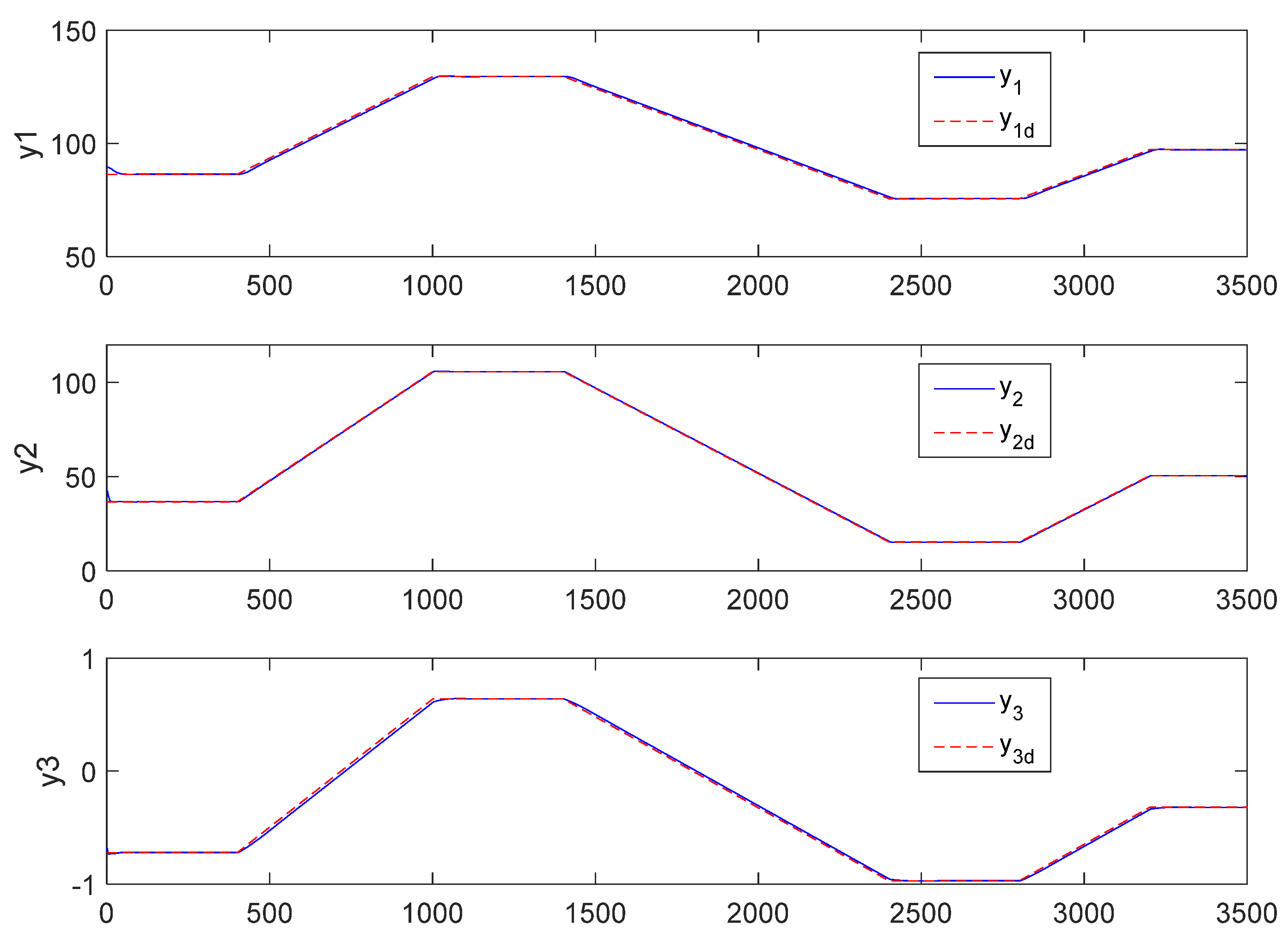
Figure 4.
Control inputs of the unit in the case of tracking large-scale load references.

Figure 5.
Estimates of lumped disturbances.

Figure 6.
Output trajectories in presence of lumped disturbances.

Figure 7.
Control inputs curves.

Figure 8.
Control outputs in presence of lumped disturbances.

Figure 9.
Control inputs in presence of lumped disturbances.

Figure 10.
The comparison results of y1 between the two controllers.

Figure 11.
The comparison results of y2 between the two controllers.

Figure 12.
The comparison results of y3 between the two controllers.

Figure 13.
The comparison results of u1 between the two controllers.

Figure 14.
The comparison results of u2 between the two controllers.

Figure 15.
The comparison results of u3 between the two controllers.


Table 1.
Model Parameters of Boiler–Turbine Unit.
Table 2.
Typical Operating Points of Boiler–Turbine Unit.
| #1 | #2 | #3 | #4 | #5 | #6 | #7 | |
|---|---|---|---|---|---|---|---|
| 75.6 | 86.4 | 97.2 | 108 | 118.8 | 129.6 | 135.4 | |
| 15.27 | 36.65 | 50.52 | 66.65 | 85.06 | 105.8 | 127 | |
| 299.6 | 324.4 | 385.2 | 428 | 470.8 | 513.6 | 556.4 | |
| 0.156 | 0.209 | 0.271 | 0.34 | 0.418 | 0.505 | 0.600 | |
| 0.483 | 0.552 | 0.621 | 0.69 | 0.759 | 0.828 | 0.897 | |
| 0.183 | 0.256 | 0.34 | 0.433 | 0.543 | 0.663 | 0.793 | |
| −0.97 | −0.65 | −0.32 | 0 | 0.32 | 0.64 | 0.98 |
Table 3.
The change process of the working condition point.
| Time Period (s) | 0–400 | 400–1000 | 1000–1400 | 1400–2400 | 2400–2700 | 2700–3200 | 3200–3500 |
|---|---|---|---|---|---|---|---|
| Working condition | #2 | #2 to #6 | #6 | #6 to #1 | #1 | #1 to #3 | #3 |
Table 4.
Quantitative integral absolute error (IAE) indexes of the simulation outputs.
| Time Frame (1) | Time Frame (2) | Time Frame (3) | Time Frame (4) | |
|---|---|---|---|---|
| Proposed method | (61.098, 63.04, 8.73) | (0.376, 26.6, 0.00105) | (0.0346,0.0472,0.000258) | (0.466, 29.64, 0.0027) |
| Galerkin control | (171.77, 72.39, 0.472) | (181.15, 219.023, 5.38) | (138.84, 165.61, 6.97) | (97.867, 39.399, 4.63) |
| State feedback control | (90.676, 60.343, 8.053) | (22.1, 25.217, 0.866) | (21.73, 6.45, 0.689) | (19.738, 25.095, 0.631) |
Table 5.
Variable of Controlled Boiler–Turbine Unit.
| Variable | ||||
|---|---|---|---|---|
| Name | identified parameter | identified parameter | identified parameter | coefficient |
| drum pressure | electrical output | fluid density in the drum | drum steam pressure | |
| electrical output | drum water level | valve positions for fuel | valve positions for steam | |
| valve positions for feedwater flow | evaporation rate of steam | unknown disturbances | setpoint signal for state | |
| w(t) | ||||
| setpoint signal for input | setpoint signal for output | disturbance term | lumped disturbance | |
| virtual control law | states/outputs error | HOSMO estimate | cost function | |
| Nth order Legendre polynomial | state variables at the LGL nodes | control variables at the LGL nodes |
Disclaimer/Publisher’s Note: The statements, opinions and data contained in all publications are solely those of the individual author(s) and contributor(s) and not of MDPI and/or the editor(s). MDPI and/or the editor(s) disclaim responsibility for any injury to people or property resulting from any ideas, methods, instructions or products referred to in the content. |
© 2023 by the authors. Licensee MDPI, Basel, Switzerland. This article is an open access article distributed under the terms and conditions of the Creative Commons Attribution (CC BY) license (https://creativecommons.org/licenses/by/4.0/).
Share and Cite
MDPI and ACS Style
Zhao, G.; Sun, Y.; Su, Z.-G.; Hao, Y. Receding Galerkin Optimal Control with High-Order Sliding Mode Disturbance Observer for a Boiler-Turbine Unit. Sustainability 2023, 15, 10129. https://doi.org/10.3390/su151310129
AMA Style
Zhao G, Sun Y, Su Z-G, Hao Y. Receding Galerkin Optimal Control with High-Order Sliding Mode Disturbance Observer for a Boiler-Turbine Unit. Sustainability. 2023; 15(13):10129. https://doi.org/10.3390/su151310129
Chicago/Turabian StyleZhao, Gang, Yuge Sun, Zhi-Gang Su, and Yongsheng Hao. 2023. "Receding Galerkin Optimal Control with High-Order Sliding Mode Disturbance Observer for a Boiler-Turbine Unit" Sustainability 15, no. 13: 10129. https://doi.org/10.3390/su151310129
Note that from the first issue of 2016, this journal uses article numbers instead of page numbers. See further details here.