
A Signal Matching Method of In-Orbit Calibration of Altimeter in Tracking Mode Based on Transponder
 ,
,
Abstract
:1. Introduction
2. Background
2.1. Altimeter

| Characteristics | Tracking Mode | Search Mode |
|---|---|---|
| Length of tracking window/m | 120 | 240 |
| Ground command switching | No | Yes |
| Preset tracking height | No | Yes |
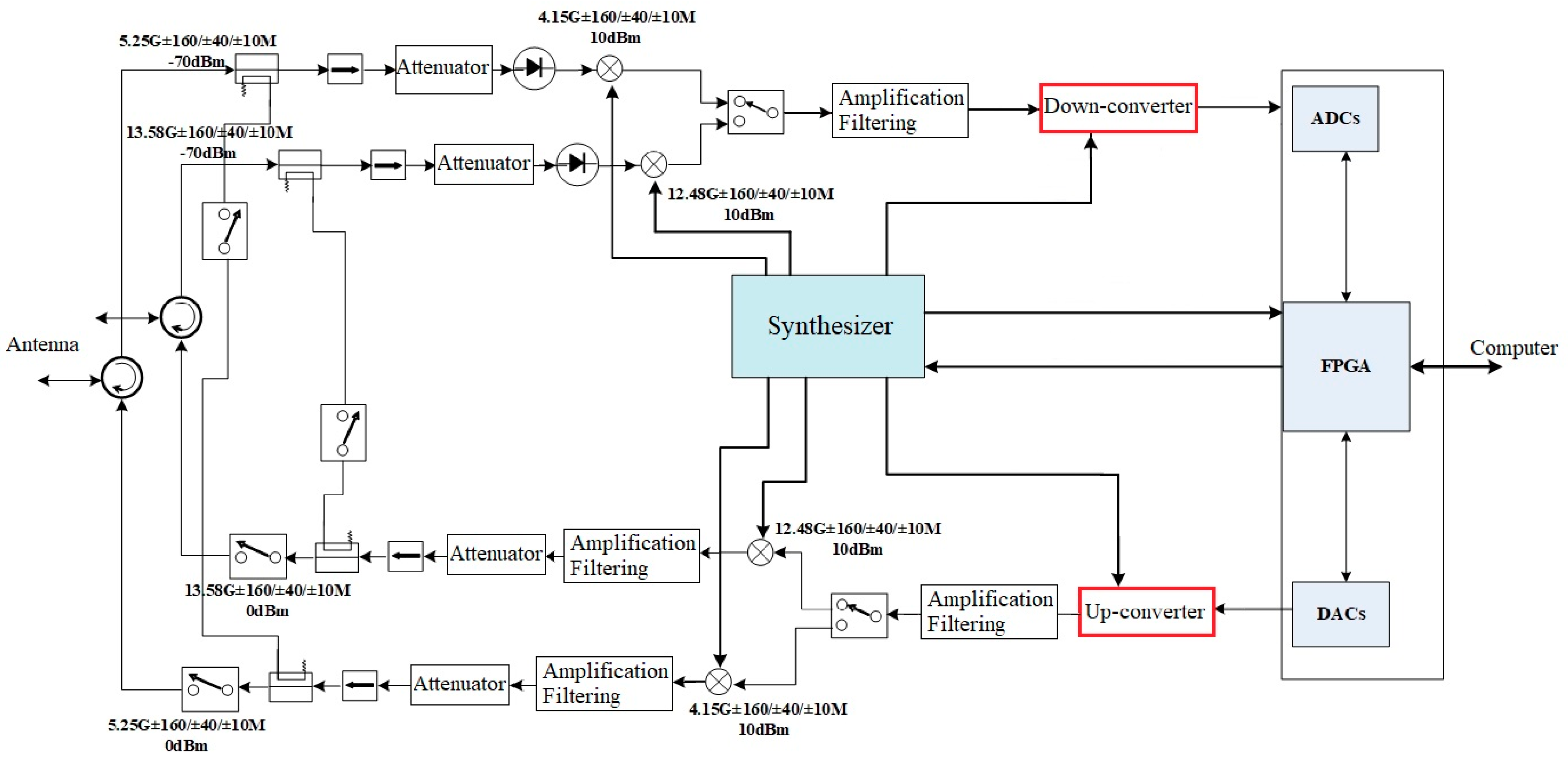
2.2. Transponder
3. Principle and Algorithm
4. Experiment and Results
5. Conclusions
Author Contributions
Funding
Data Availability Statement
Acknowledgments
Conflicts of Interest
References
- Pesec, P.; Sünkel, H.; Windholz, N. The Use of Transponders in Altimetry. In Gravity and Geoid: Joint Symposium of the International Gravity Commission and the International Geoid Commission; Sünkel, H., Marson, I., Eds.; Springer: Berlin/Heidelberg, Germany, 1995; Volume 113, pp. 394–400. [Google Scholar]
- Mertikas, S.P.; Donlon, C.; Mavrocordatos, C.; Piretzidis, D.; Kokolakis, C.; Cullen, R.; Matsakis, D.; Borde, F.; Fornari, M.; Boy, F.; et al. Performance evaluation of the CDN1 altimetry Cal/Val transponder to internal and external constituents of uncertainty. Adv. Space Res. 2022, 70, 2458–2479. [Google Scholar] [CrossRef]
- Mertikas, S.P.; Donlon, C.; Kokolakis, C.; Piretzidis, D.; Cullen, R.; Féménias, P.; Fornari, M.; Frantzis, X.; Tripolitsiotis, A.; Bouffard, J.; et al. The ESA Permanent Facility for Altimetry Calibration in Crete: Advanced Services and the Latest Cal/Val Results. Remote Sens. 2024, 16, 223. [Google Scholar] [CrossRef]
- Mertikas, S.P.; Donlon, C.; Féménias, P.; Mavrocordatos, C.; Galanakis, D.; Tripolitsiotis, A.; Frantzis, X.; Tziavos, I.N.; Vergos, G.; Guinle, T. Fifteen Years of Cal/Val Service to Reference Altimetry Missions: Calibration of Satellite Altimetry at the Permanent Facilities in Gavdos and Crete, Greece. Remote Sens. 2018, 10, 1557. [Google Scholar] [CrossRef]
- Garcia-Mondéjar, A.; Fornari, M.; Bouffard, J.; Féménias, P.; Roca, M. CryoSat-2 range, datation and interferometer calibration with Svalbard transponder. Adv. Space Res. 2018, 62, 1589–1609. [Google Scholar] [CrossRef]
- Guo, W.; Gong, X.-Y.; Xu, X.-Y.; Liu, H.-G.; Xu, C.-D.; Du, Y.-H. A transponder system dedicating for the on-orbit calibration of China’s new-generation satellite altimeter and scatterometer. In Proceedings of the 2011 IEEE CIE International Conference on Radar, Chengdu, China, 24–27 October 2011; pp. 22–25. [Google Scholar]
- Wang, C.; Guo, W.; Zhao, F.; Wan, J.; Xu, K. Development of the reconstructive transponder for in-orbit calibration of HY-2 altimeter. In Proceedings of the 2015 IEEE International Geoscience and Remote Sensing Symposium (IGARSS), Milan, Italy, 26–31 July 2015; pp. 3645–3648. [Google Scholar]
- Xu, X.-Y.; Guo, W.; Liu, H.-G.; Shi, L.-W.; Lin, W.-M.; Du, Y.-H. Design of the interface of a calibration transponder and an altimeter/scatterometer. In Proceedings of the 2011 IEEE International Geoscience and Remote Sensing Symposium, Vancouver, BC, Canada, 24–29 July 2011; pp. 953–956. [Google Scholar]
- Wan, J.; Guo, W.; Zhao, F.; Wang, C.; Liu, P. HY-2A Radar Altimeter Ultrastable Oscillator Drift Estimation Using Reconstructive Transponder with Its Validation by Multimission Cross Calibration. IEEE Trans. Geosci. Remote Sens. 2015, 53, 5229–5236. [Google Scholar] [CrossRef]
- Wang, C.; Guo, W.; Zhao, F.; Wan, J.; Liu, P.; Lin, M.; Peng, H.; Xu, C. Development of the Reconstructive Transponder for In-Orbit Calibration of HY-2A Altimeter. IEEE J. Sel. Top. Appl. Earth Obs. Remote Sens. 2016, 9, 2709–2719. [Google Scholar] [CrossRef]
- Wan, J.; Guo, W.; Zhao, F.; Wang, C. Echo signal quality analysis during HY-2A radar altimeter calibration campaign using reconstructive transponder. In Proceedings of the 2015 IEEE International Geoscience and Remote Sensing Symposium (IGARSS), Milan, Italy, 26–31 July 2015; pp. 3652–3654. [Google Scholar]
- Wan, J.; Guo, W.; Wang, C.; Zhao, F. A Matching Method for Establishing Correspondence between Satellite Radar Altimeter Data and Transponder Data Generated during Calibration. IEEE Geosci. Remote Sens. Lett. 2014, 11, 2145–2149. [Google Scholar]
- Xu, K.; Liu, P.; Tang, Y.; Yu, X. The improved design for HY-2B radar altimeter. In Proceedings of the 2017 IEEE International Geoscience and Remote Sensing Symposium (IGARSS), Fort Worth, TX, USA, 23–28 July 2017; pp. 534–537. [Google Scholar]
- Wang, C.; Guo, W.; Liu, P.; Wang, T.; Cui, H. In-Orbit Calibration and Validation of HY-2B Altimeter using an Improved Transponder. In Proceedings of the IGARSS 2020—2020 IEEE International Geoscience and Remote Sensing Symposium, Waikoloa, HI, USA, 26 September–2 October 2020; pp. 5819–5822. [Google Scholar]
- Wang, C.; Guo, W.; Liu, P.; Wang, T. Development and Integration Test of an Improved Transponder for Hy–2B Altimeter. In Proceedings of the IGARSS 2020—2020 IEEE International Geoscience and Remote Sensing Symposium, Waikoloa, HI, USA, 26 September–2 October 2020; pp. 5862–5865. [Google Scholar]
- Xu, K.; Jiang, J.; Liu, H. A new tracker for ocean-land compatible radar altimeter. In Proceedings of the 2007 IEEE International Geoscience and Remote Sensing Symposium, Barcelona, Spain, 23–28 July 2007; pp. 3825–3828. [Google Scholar]
- Wan, J. Study on HY-2 Altimeter System Delay In-Orbit Absolute Calibration Using Reconstructive Transponder. Ph.D. Thesis, The University of Chinese Academy of Sciences and National Space Science Center, Chinese Academy of Sciences, Beijing, China, 2015. [Google Scholar]
- Cui, H.; Guo, W.; Wang, C.; Wang, T. In Orbit Test of Clock Frequency Deviation of HY-2B Satellite Radar Altimeter based on Transponder. Remote Sens. Technol. Appl. 2021, 36, 581–586. [Google Scholar]
- Kalata, P.R. α-β target tracking systems: A survey. In Proceedings of the 1992 American Control Conference, Chicago, IL, USA, 24–26 June 1992; pp. 832–836. [Google Scholar]
- Brown, G. The average impulse response of a rough surface and its applications. IEEE J. Ocean. Eng. 1977, 2, 67–74. [Google Scholar] [CrossRef]


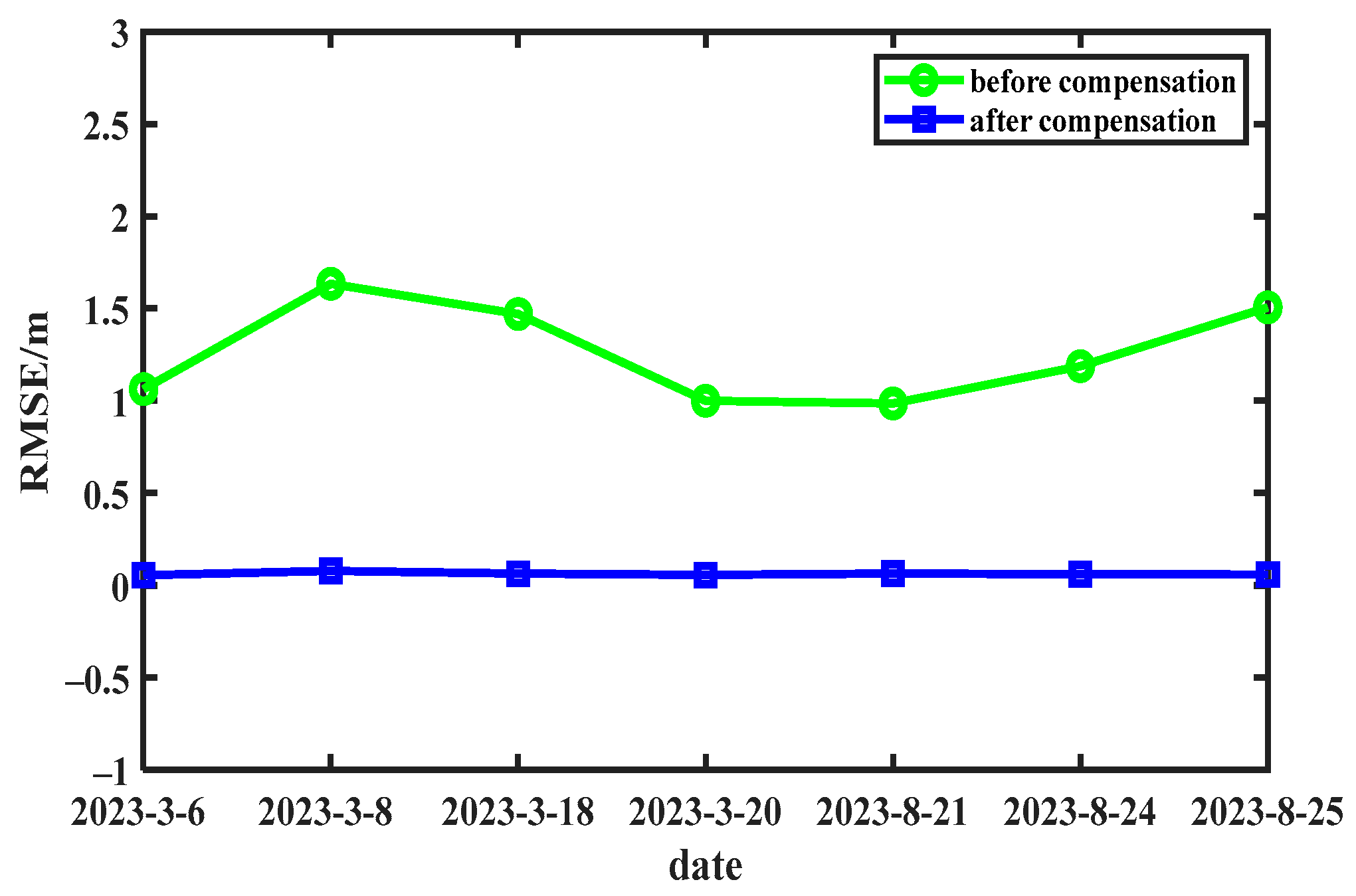
| Satellite | Date | Before Compensation (m) | After Compensation (m) |
|---|---|---|---|
| HY-2B | 6 March 2023 | 1.0632 | 0.0546 |
| HY-2D | 8 March 2023 | 1.6342 | 0.0788 |
| HY-2D | 18 March 2023 | 1.4708 | 0.0629 |
| HY-2B | 20 March 2023 | 0.9996 | 0.0566 |
| HY-2B | 21 August 2023 | 0.9852 | 0.0643 |
| HY-2D | 24 August 2023 | 1.1882 | 0.0609 |
| HY-2C | 25 August 2023 | 1.5068 | 0.0582 |
Disclaimer/Publisher’s Note: The statements, opinions and data contained in all publications are solely those of the individual author(s) and contributor(s) and not of MDPI and/or the editor(s). MDPI and/or the editor(s) disclaim responsibility for any injury to people or property resulting from any ideas, methods, instructions or products referred to in the content. |
© 2024 by the authors. Licensee MDPI, Basel, Switzerland. This article is an open access article distributed under the terms and conditions of the Creative Commons Attribution (CC BY) license (https://creativecommons.org/licenses/by/4.0/).
Share and Cite
Fang, Q.; Guo, W.; Wang, C.; Liu, P.; Wang, T.; Han, S.; Yang, S.; Zhang, Y.; Peng, H.; Ma, C.; et al. A Signal Matching Method of In-Orbit Calibration of Altimeter in Tracking Mode Based on Transponder. Remote Sens. 2024, 16, 1682. https://doi.org/10.3390/rs16101682
Fang Q, Guo W, Wang C, Liu P, Wang T, Han S, Yang S, Zhang Y, Peng H, Ma C, et al. A Signal Matching Method of In-Orbit Calibration of Altimeter in Tracking Mode Based on Transponder. Remote Sensing. 2024; 16(10):1682. https://doi.org/10.3390/rs16101682
Chicago/Turabian StyleFang, Qingyu, Wei Guo, Caiyun Wang, Peng Liu, Te Wang, Sijia Han, Shijie Yang, Yufei Zhang, Hailong Peng, Chaofei Ma, and et al. 2024. "A Signal Matching Method of In-Orbit Calibration of Altimeter in Tracking Mode Based on Transponder" Remote Sensing 16, no. 10: 1682. https://doi.org/10.3390/rs16101682