Article

Assessment of Passive Solar Heating Systems’ Energy-Saving Potential across Varied Climatic Conditions: The Development of the Passive Solar Heating Indicator (PSHI)

1
Faculty of Environmental Engineering, The University of Kitakyushu, Kitakyushu 808-0135, Japan
2
School of Civil Engineering and Architecture, Zhejiang University of Science & Technology, Hangzhou 310023, China
3
Zhejiang Southeast Architectural Design Group Co., Ltd., Hangzhou 310023, China
4
School of Art and Design, Xi’an University of Technology, Xi’an 710054, China
5
Graduate School of Information, Production and Systems, Waseda University, Kitakyushu 808-0135, Japan
*
Author to whom correspondence should be addressed.
Buildings 2024, 14(5), 1364; https://doi.org/10.3390/buildings14051364
Submission received: 20 March 2024 / Revised: 28 April 2024 / Accepted: 7 May 2024 / Published: 10 May 2024

Abstract

:
This study aims to evaluate the energy-saving potential of passive solar heating systems in diverse global climates and introduce a new indicator, the passive solar heating indicator (PSHI), to enhance the efficiency of building designs. By collecting climate data from 600 cities worldwide through a simulation model, the present study employs polynomial regression to analyze the impact of outdoor temperature and solar radiation intensity on building energy savings. It also uses K-means cluster analysis to scientifically categorize cities based on their energy-saving potential. The findings underscore the benefits of both direct and indirect solar heating strategies in different climates. Significantly, the PSHI shows superior predictive accuracy and applicability over traditional indices, such as the irradiation temperature difference ratio (ITR) and the irradiation degree hour ratio (C-IDHR), especially when outdoor temperatures are close to indoor design temperatures. Moreover, the application of a cluster analysis provides hierarchical guidance on passive heating designs globally, paving the way for more accurate and customized energy-efficient building strategies.

1. Introduction

1.1. Motivation

Reducing energy consumption and carbon emissions from buildings is pivotal in addressing the challenges of global energy usage and climate change. A data report [1] indicates that buildings account for 35% of worldwide energy consumption and about one-third of total carbon emissions. Specifically, during the heating season, the building sector consumes approximately 20% of primary energy and 23% of electricity [2,3,4,5,6,7]. In response, the development and implementation of zero-carbon building solutions, especially those that incorporate solar heating technologies, have become essential in achieving energy efficiency and emission reduction objectives [8,9,10,11,12,13].
Numerous scholars have focused on researching active solar heating systems (ASHSs) and passive solar heating systems (PSHSs) to reduce building heating energy consumption [14,15]. Unlike ASHSs, which use mechanical equipment such as solar water heaters and air heating systems, PSHSs operate without additional energy, attracting significant research and practical interest [16,17]. During the initial stages of architectural design, assessing the solar energy resources at the site is crucial to predict a PSHS’s energy-saving effects and determine the suitability of a direct-benefit (PSHS-d) or indirect-benefit (PSHS-in) system. China’s solar resource zoning standards [18] divide the country into several regions according to solar radiation intensity; however, this standard does not account for the impact of the temperature difference between the indoor heating design temperature and the outdoor average temperature on heating energy efficiency. Setting an indoor heating temperature means that if external temperatures are lower, the greater indoor–outdoor temperature difference will increase heat loss and require more energy to maintain indoor warmth. Consequently, in regions with high heating needs, using solar energy to heat indoor air can significantly reduce energy consumption. To address this need, indices like the ITR [19] and C-IDHR [20] were developed. The ITR categorizes regions empirically based on the ratio of the average solar radiation facing south during the coldest month to the temperature difference between the indoor heating design temperature and the outdoor average temperature. The C-IDHR is calculated by dividing the solar radiation intensity by the temperature difference when outdoor temperatures fall below the indoor design temperature. While these indices are useful, further exploration is needed to address the following issues:
  • When outdoor temperatures are close to the indoor design temperature, does the method of calculating energy efficiency by dividing solar radiation intensity by the temperature difference remain effective?
  • Do the energy-saving potentials of direct-benefit (PSHS-d) and indirect-benefit (PSHS-in) systems consistently align?
  • Is there a more scientific and effective method to delineate the energy-saving potential zones of PSHSs?
Therefore, developing an efficient method to refine the passive solar heating indicator (PSHI) is essential for accurately assessing the energy-saving potential of PSHSs in buildings across various regions. This study aims to refine the indicator for passive heating potential by simulating the heating energy savings achievable in buildings across 600 cities worldwide, thus creating an extensive database for polynomial regression analysis. It designates outdoor temperature and solar radiation intensity as independent variables and building energy savings as the dependent variable. This approach aids in establishing a relational equation between the PSHI and these crucial variables. Finally, this study utilizes K-means cluster analysis to categorize cities based on their PSHI, providing valuable insights for designing passive heating systems in buildings.

1.2. Literature Review

This study sheds light on the process of evaluating and grading the energy-saving potential of passive solar heating systems (PSHSs). Traditionally, solar radiation intensity has been recognized as a pivotal factor in gauging the efficiency of PSHSs. In China, existing building standards provide a methodical approach for analyzing the feasibility of solar energy use in buildings, and newer regulations [18] have introduced a system of solar energy zoning based on the accessibility of solar radiation resources. As a result, this measure has become integral in assessing the efficiency of PSHSs.
Nevertheless, recent advancements in design practices, especially in the creation of efficient PSHSs that do not rely on external heat sources, have shifted the focus toward the combined impacts of solar radiation and temperature differences [21,22]. This approach evaluates solar heating effectiveness by considering both solar irradiation levels and the differential between indoor and outdoor temperatures, referred to as the ITR. Building on this concept, Meng et al. [14] have developed the C-IDHR, which uses an hour-by-hour accumulation strategy to classify regional solar heating potential.
Polynomial regression (PR) models have become indispensable in predicting and optimizing the performance of complex systems across various fields of scientific research [23,24,25,26,27]. In the realm of environmental engineering, multivariate polynomial regression (MPR)-based models have proven effective in delivering rapid and accurate predictions for systems such as dew point cooling (DPC) by utilizing comprehensive data analyses [28]. Furthermore, PR models have demonstrated their capability in accurately predicting the energy value conversion from poultry waste, paving the way for innovative biomass energy conversion solutions [29].
The application of PR models extends beyond environmental engineering and energy sectors, finding relevance in areas such as marketing and water management [30,31]. Notably, research [32] has shown that integrating PR models with K-means clustering significantly improves the precision of predictions concerning pipeline failures in water supply networks. K-means clustering has also been effectively applied in various fields, including the classification of industrial accidents [33], water pollution [34], urban waste [35], and building sub-zoning [36], further exemplifying the versatility and effectiveness of these analytical tools.

1.3. Scientific Originality

The innovation lies in its methodical expansion to evaluate energy savings of PSHSs across diverse climatic conditions in 600 cities globally, extending beyond the typical focus on specific locations or climates to provide a global perspective.
Using polynomial regression with outdoor temperature and solar radiation as independent variables enhances the connection between the PSHI and environmental factors, thus improving the precision of energy-saving predictions.
The development of the PSHI enables us to uniquely identify performance differences between direct-benefit (PSHS-d) and indirect-benefit (PSHS-in) passive solar heating systems across diverse climates. This innovation addresses existing gaps in accurately assessing the efficacy of various systems.
Applying K-means cluster analysis to scientifically classify cities by their PSHI, we can recognize and utilize urban diversity to tailor more precise PSHS applications.

1.4. Aims of This Research

This work is dedicated to thoroughly analyzing and refining passive heating strategies by creating a polynomial regression model-based PSHI and methodically categorizing these indicators through K-means clustering. Our goal is to dissect the temperature thresholds critical for the efficacy of the PSHS-d, employing indicators to pinpoint the precise temperatures at which passive heating yields substantial energy savings in diverse climatic conditions.
We set out to model the interplay between the potential for energy savings in buildings and pivotal environmental variables, specifically temperature and solar radiation intensity. This approach aims to elucidate the joint influence of these factors on passive heating effectiveness.
Furthermore, our objective includes devising a passive heating potential indicator that is responsive across a wider range of temperatures. This enhancement will facilitate a more comprehensive evaluation of PSHSs in varied climatic scenarios.
The culminating aim of this research is to define the gradations of the PSHI and its respective thresholds, grounded on empirical data. Through K-means cluster analysis, we plan to scientifically classify cities based on their capacity for energy savings via PSHSs. This structured classification will enable a targeted application of PSHSs, tailored to the specific energy-saving potential of different urban environments.

2. Methodology

2.1. Source of Climate Data

This study harnesses climatic datasets from two pre-eminent sources widely recognized in the realm of building performance simulation: the EnergyPlus Weather data [37] and One Building database [38]. These sources are acclaimed internationally for their contribution to building science research and their utility in practical applications, providing comprehensive climate baseline data essential for energy simulations and performance evaluations at every scale—from individual buildings to expansive urban areas.
Drawing on these reputable databases, climate data for over 600 cities across various major geographic regions were meticulously compiled, as illustrated in Figure 1. This dataset encompasses detailed hourly climate parameters for each city, including temperature, humidity, and solar radiation intensity. These parameters are derived from long-term observational records and are subject to strict quality control measures to ensure their reliability and accuracy.
The wide-reaching coverage and high precision of these datasets furnish a globally representative and applicable base for analysis within this study. Through methodical examination of these climate data, this study sets out to develop a novel model for gauging the passive heating potential. This endeavor aims to provide a more accurate and practical instrument for designing energy-efficient buildings, enhancing the ability to tailor building designs to optimize energy savings and performance based on specific climate conditions.

2.2. Definition of Different Indicators of Solar Heating Potential

2.2.1. Equation Analysis of ITR Indicator

The ITR is a crucial metric for assessing building energy efficiency, especially regarding PSHSs. Defined as the average daily solar radiation from the southern exposure divided by the temperature difference between indoor and outdoor environments during the year’s coldest month, the ITR is vital for optimizing natural light and heat. This period usually sees the highest heating demands, and effective solar radiation utilization can significantly lower energy needs. Architects and environmental engineers use the ITR in designing energy-efficient buildings while ensuring thermal comfort. The ITR can be calculated using Equation (1):
I T R = H ¯ t v s , 1 min T a T ¯ o , 1 min
where H ¯ t v s , 1 min is the mean daily global solar radiation on the south surface in the coldest month (Wm−2), T a is the indoor base temperature (°C), and T ¯ o , 1 min is the mean daily outdoor temperature in the coldest month (°C). T a T ¯ o , 1 min should be positive.

2.2.2. Equation of C-IDHR Indicator

The C-IDHR is a metric developed to evaluate the potential of solar heating. It functions as a preliminary step to ascertain whether the temperature differential between indoor and outdoor environments exceeds zero, a critical consideration before incorporating solar radiation values into the assessment. The formulation of the C-IDHR involves a series of equations, specifically Equations (2)–(4):
I D H R = H N , h p H D H h p
H N , h p = i = h p s , 1 h h p H N , i × s i g n 15 T o , i h s i g n ( 15 T o , i h ) 1,15 T o , i h > 0 0,15 T o , i h 0
H D   H h p = i = h p s , 1 h h p ( 15 T o , i h ) × ( 15 T o , i h )
where H D   , h p is the cumulative hourly solar radiation value for the heating period (HP) (Wm−2), and H D   H h p is the temperature difference between the indoor base temperature and the outdoor air temperature.

2.3. Definition and Calculation of PSHI

2.3.1. Building Geometry

This research assesses the influence of PSHSs on the heating energy consumption of buildings situated in diverse climatic zones. By conducting a simulation and analysis on three distinct building models, this study illuminates the energy-saving capabilities of both the PSHS-d and PSHS-in. Researchers frequently use an ideal room as a building model to demonstrate the energy savings provided by PSHSs across various climates [39,40,41,42]. In this context (as Figure 2 shows), Building A serves as the baseline model, with dimensions of 4 m × 6 m × 3.4 m and a south-facing window-to-wall ratio of 0.3, replicating the heating demand of a typical residential building. Building B, while maintaining the same dimensions, features an increased window-to-wall ratio of 0.5. This adjustment aims to explore the energy efficiency of the PSHS-d, highlighting the advantages of straightforward and effective solar access [43,44,45,46]. Building C is designed to assess the efficacy of a PSHS-in, incorporating a Trombe wall [47,48,49,50] to leverage its reliable thermal insulation properties. Simulation experiments, employing accurate climatic data, were conducted to compare the heating energy requirements under different PSHSs for these models.
To guarantee the adaptability and precision of the models, particularly since a building’s winter heating demand is contingent on outdoor temperature, solar radiation, and specific building parameters like an envelope and PSHSs, this study utilized the ASHRAE Thermal Zoning Guidelines. These guidelines helped in selecting code-compliant envelope materials for each model (as Table 1 shows), ensuring optimal building performance across various climates. Table 2 in this study meticulously outlines the interior health gains (such as equipment power, lighting power, and occupant density) and other parameters employed in the analysis. Figure 3 illustrates the tools used for the experiments.

2.3.2. Polynomial-Based Regression Models

This study proposes the adoption of a polynomial regression model for the heating energy saving potential indicator. This model is better suited to accurately depict the complex nonlinear relationships between environmental factors—such as temperature and solar radiation intensity—and the potential for energy savings in buildings.
Polynomial regression excels in managing nonlinear relationships, thereby effectively establishing a correlation between environmental variables and the potential for building energy savings. This method stands out for its simplicity and interpretability compared to more complex models like neural networks, making it easier to identify critical factors that influence energy-saving potential and to devise effective energy-saving strategies. The strength of polynomial regression lies in its ability to linearly relate to its coefficients, gaining its versatility from the power to approximate functions through polynomials.
In light of the focus on two key environmental parameters, temperature and solar radiation intensity, this study employs a binary polynomial regression model. This model is characterized by the following equation:
y = β 0 + β 1 x 1 + β 2 x 2 + β 3 x 1 2 + β 4 x 1 x 2 + β 5 x 2 2 + β 6 x 1 2 x 2 + β 7 x 1 x 2 2 + + ϵ
Here, y is the dependent variable, x1 and x2 are the independent variables, β0, β1, …, represent the model parameters, and ϵ denotes the error term.
This research aims to investigate eight distinct fitting scenarios to assess the energy-saving potential of PSHSs comprehensively. These scenarios are categorized based on two primary environmental factors: solar radiation intensity and temperature. For solar radiation, this study will examine the impact of both southward-facing solar radiation intensity and the total solar radiation intensity on the building’s passive heating potential. Regarding temperature, the analysis will focus on two aspects: the average outdoor temperature during the heating period and the differential between the indoor heating design temperature and the average outdoor temperature.

2.3.3. Statistical Metrics for Analyzing Polynomial Fits

This study applies polynomial function fitting to delve into the energy-saving potential of PSHSs within buildings. To quantitatively evaluate the effectiveness of the fit, this study employs two statistical metrics: the coefficient of determination (R2) and the mean square error (MSE). R2, which ranges from 0 to 1, is used to compare the goodness-of-fit among various models, with values closer to 1 denoting a model’s enhanced capability to explain the variability in the data. On the other hand, MSE quantifies the average of the squares of the differences between the predicted and observed values, serving as an indicator of the model’s prediction accuracy. Lower values of MSE are indicative of higher accuracy. The calculations for R2 and MSE are as follows:
R 2 = 1 y i y ^ i 2 y i y ¯ 2
M S E = 1 n i = 1 n y i y ^ i 2
where yi is the ith observed value, yi is the ith predicted value, y is the average of the observed values, and n is the total number of observations.

2.3.4. Indicator Classification for K-Means-Based Cluster Analysis

In this investigation, the fitted polynomial model was employed to categorize passive solar heating potential indicators through K-means cluster analysis. K-means is a type of unsupervised learning algorithm that aims to enhance clustering quality by minimizing the Euclidean distance, denoted as L. This method effectively groups samples with high similarity into the same cluster, facilitating the analysis of data with inherent groupings but without pre-labeled classifications.
The algorithm achieves this by dividing the dataset into k distinct clusters, where k represents the predetermined number of clusters. It ensures that each data point in the dataset is nearest to the centroid of its cluster. The centroid is essentially the center point of a cluster, calculated as the mean position of all of the points in the cluster. This process iteratively adjusts the positions of the centroids and the assignment of data points to clusters until an optimal grouping is achieved, where the total intra-cluster variation (or the sum of the Euclidean distances between the data points and their respective cluster centroid) is minimized.
The Euclidean distance, which is a measure of the straight line distance between two points in Euclidean space, is defined by the following formula:
L = x m i 2
m i = 1 n i = 1 n x i ,
Here, x represents the data sample points, mi is the center of cluster i (centroid), n is the number of data samples within cluster m.
In cluster analysis, evaluating the performance of clustering involves using metrics such as the sum of squared errors (WCSS). WCSS measures the coherence of clusters by calculating the sum of the squared distances between each sample and its cluster center, essentially assessing each sample’s similarity to its cluster centroid and summing these squared differences. A general principle is that as the number of clusters increase, WCSS tends to decrease because the clusters become tighter, indicating a reduction in the dispersion among clusters. This relationship is captured in the following algorithmic expression:
W C S S = i = 1 k x C i L
Here, k represents the number of clusters, Ci denotes the ith cluster, x signifies the point within cluster i, and mi is the centroid of cluster Ci.
Initially, with an increase in the number of clusters, WCSS usually shows a downward trend. However, after reaching a certain threshold, the decrease in WCSS begins to plateau, indicating that adding more clusters does not significantly reduce the distance between the points and their respective centroids.
To identify the optimal number of clusters, the elbow rule is applied. This involves looking for an inflection point on the WCSS versus the number of clusters graph. Beyond this inflection point, the rate of decrease in WCSS becomes less significant, creating an “elbow” shape on the graph. Identifying this point helps ascertain the most appropriate number of clusters for the dataset. Once the optimal number of clusters are determined, the centroid of each cluster is calculated. The arithmetic mean of the centroids of adjacent clusters in the one-dimensional feature space then becomes the threshold for distinguishing between clusters.

3. Result and Analysis

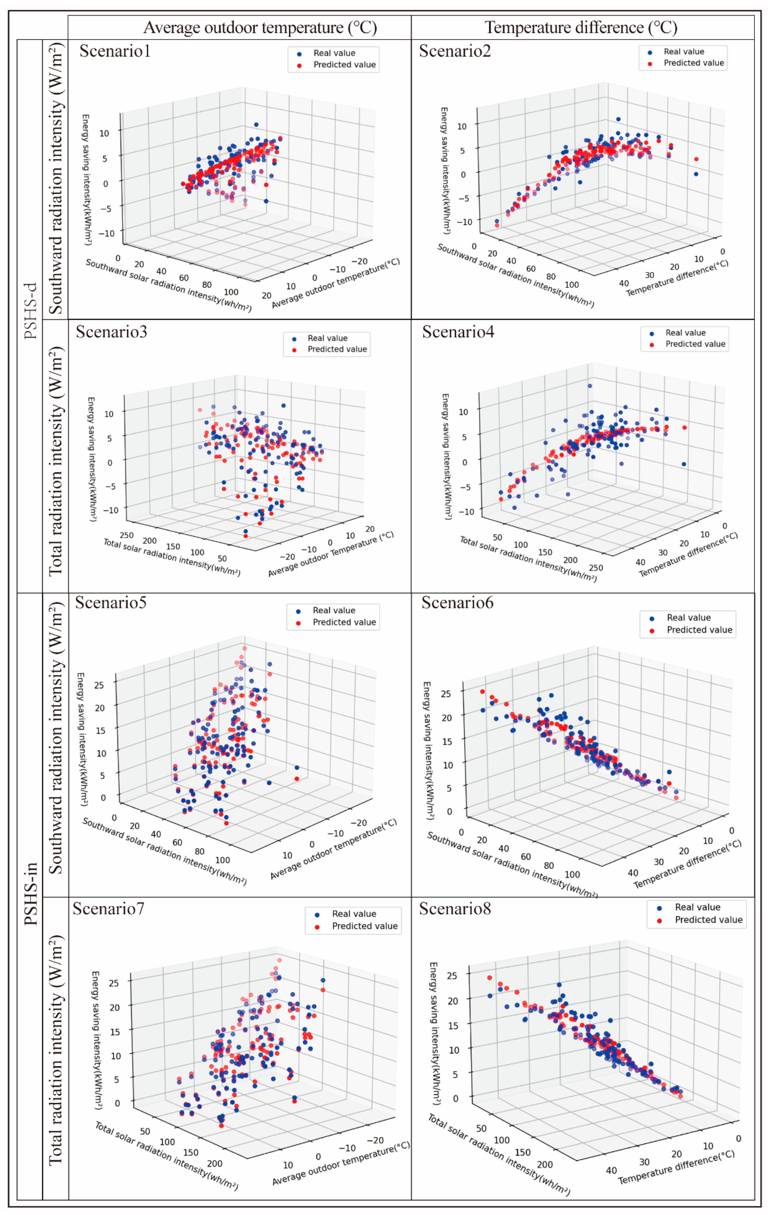
3.1. Relationship between Energy-Saving Potential and Single Factors

This section delves into the energy-saving efficacy of both the PSHS-d and PSHS-in, exploring how various factors—outdoor temperature, the differential between indoor and outdoor temperatures, total solar radiation, and south-facing solar radiation—affect the potential for energy savings. The investigation reveals that, contrary to expectations, the distribution of data pertaining to the PSHS-d does not exhibit an inverse proportional relationship.
As illustrated in Figure 4, the colored dots represent the energy-saving potential at each data point, with deeper colors indicating higher energy-saving potential and lighter colors representing lower energy-saving potential. the correlation between building energy savings and the average outdoor temperature showcases a parabolic trajectory. The apex of energy savings is observed when the average outdoor temperature is around −0.6 °C. Below this pivotal temperature, a decline in outdoor temperature corresponds with diminished building energy savings, and conversely, an elevation in outdoor temperature also leads to a reduction in savings. In regions with low temperatures, the solar energy captured by the PSHS-d is insufficient to offset the heat loss at night. Conversely, in warmer regions with lower heating demands, the PSHS-d does not yield significant energy savings. This pattern is indicative of the PSHS-d’s approach to augmenting the window-to-wall ratio, which enhances solar radiation absorption and aims to increase indoor temperatures during daylight hours, thereby reducing the necessity for heating.
However, the effectiveness of the PSHS-d in promoting energy savings is limited in colder climates due to the augmented heat loss at night through windows. Despite their role in facilitating solar gain, windows are not as thermally insulating as walls, leading to greater energy loss in such environments. Conversely, in regions with higher temperatures, the contribution of solar heating strategies to energy savings is negligible, given the already low demand for heating in these areas.

3.2. Polynomial Fitting Results for Different Scenarios

In this comprehensive analysis, 70% of the data from 600 cities on heating energy savings under the PSHS were used as the training set to develop the polynomial, and the remaining 30% were used as the test set to verify the polynomial’s accuracy. This study explores eight distinct scenarios, focusing on models that predict indoor temperatures for both the PSHS-d and PSHS-in. These models take into account various factors such as the average outdoor temperature, the difference between indoor and outdoor temperatures, and the intensity of solar radiation. The PSHS-d covered in scenarios 1 through 4 highlights the immediate effect of solar radiation. In contrast, the PSHS-in encapsulated in scenarios 5 through 8 may give more weight to the outdoor temperature.
The findings (as shown in Table 3) reveal that models based on the PSHS-in generally achieve higher R2 values and a lower mean square error (MSE) across most scenarios, pointing to superior predictive accuracy. This suggests that the PSHS-in is more effective in capturing the nuances of how environmental factors influence indoor temperatures. Nonetheless, it is noteworthy that scenarios 3 and 4, which are part of the PSHS-d, register relatively lower R2 values and a higher MSE. This implies that in these scenarios, the effects of the indoor–outdoor temperature difference and solar radiation intensity on predicting indoor temperatures may not be as significant as the influence of other variables. Based on R2 and MSE, the fitting models for scenario 1 and scenario 5 were chosen as the polynomial model’s result.
Scatter plots (Figure 5) serve as visual aids, offering an intuitive understanding of the relationship between predicted values and actual observations. These plots are particularly illustrative in the context of the PSHS-in, where the strength of the relationship between predictions and actual indoor temperatures is clearly demonstrated. This visual evidence reinforces the statistical findings, highlighting the PSHS-in’s enhanced ability to accurately predict indoor temperatures based on the examined environmental factors.

3.3. Comparison of ITR, C-IDHR, and PSHI

3.3.1. Global Distribution of Indicators

Utilizing equations to compute passive solar heating potential indicators like the ITR and C-IDHR, this study paints a global picture of PSHSs’ potential on a world map (as shown in Figure 6). The analysis employs quantitative metrics to evaluate the effectiveness of PSHSs across diverse latitudes and regions, with darker colors on the graphs indicating superior heating outcomes. Each point of origin marks the lower value threshold for each heating metric, providing a visual guide to the potential applicability of PSHSs worldwide.
The ITR metric, which assesses the proportion of heat energy from solar radiation relative to a building’s heating demand, highlights the effectiveness of passive solar heating by considering solar radiation intensity and the indoor–outdoor temperature difference during winter. Areas near the equator show higher ITR values, benefiting from intense solar radiation and minor temperature differences, signaling effective heating capabilities in these regions.
In contrast, the C-IDHR metric focuses on direct solar radiation heating hours, excluding periods when outdoor temperatures rise above the indoor heating design temperature. This metric suggests that areas with high C-IDHR values are those where direct solar radiation is prevalent and temperatures remain below 18 °C. However, lower C-IDHR values at approximately 20° latitude indicate that despite favorable ITR conditions, the effectiveness of solar radiation for heating is reduced when daytime outdoor temperatures exceed the indoor heating design threshold.
The PSHI-d evaluates the direct utilization of solar radiation for heating. Notably, regions above 40° N latitude are highlighted as particularly suitable for the PSHS-d due to favorable climatic and solar radiation conditions. Yet, areas above 60° N face limitations under extreme winter conditions, aligning with findings from previous studies [46]. The difference lies in that this study extends over a broader range of areas and shows that from a baseline of 40° N, decreasing latitude corresponds with rising temperatures, while increasing latitude leads to colder temperatures and more pronounced attenuation of the PSHI-d. In high-latitude, low-temperature regions, the solar energy captured by the PSHS-d is insufficient to offset the heat loss, so the PSHS-d is not recommended in those regions.
Moreover, the PSHI-in demonstrates a close correlation with latitude. Darker shades near the North Pole and lighter shades toward the equator reflect the impact of the PSHS-in, which focuses on enhancing thermal insulation for improved heat retention and utilization of solar radiation in colder climates. Consequently, colder regions exhibit higher PSHI-in values, emphasizing the significance of building insulation and solar radiation management for heating purposes, especially in harsh winter conditions.
This comprehensive analysis, represented through a series of maps, juxtaposes global variations in passive solar heating potential across different evaluation metrics. While the ITR metric may overlook specific local climatic nuances, affecting its broad applicability, the C-IDHR metric addresses this by discounting periods of excessive outdoor temperatures. Similarly, the PSHI-d metric underscores the geographical suitability of the PSHS-d, whereas the PSHI-in metric showcases the pronounced benefits of the PSHS-in in reducing energy consumption through enhanced insulation and solar utilization in colder climates.

3.3.2. Comparison of ITR, C-IDHR, and PSHI-d

To assess the predictive power of each indicator for heating energy savings more effectively, the ITR, C-IDHR, and PSHI-d were calculated for seven representative cities, as depicted in the accompanying figure. The graph illustrates the efficacy of the PSHI-d across these cities by including data on the C-IDHR, ITR, heating degree day (HDD18 °C), and south-facing solar radiation intensity, as show in Figure 7.
Despite the varying climates of Harbin and Chengdu, both cities show PSHI-in values of 0. Harbin experiences a significantly colder climate, with temperatures averaging at 14.77 °C and a higher heating degree day count of 5497 °Cd, along with greater southwardsolar radiation (65.28 Wh/m2) compared to Chengdu’s 25.32 Wh/m2. This suggests that Harbin’s solar gains are likely nullified by night-time losses, eliminating the benefits of daytime energy savings. Conversely, Chengdu’s warmer climate does not compensate for its low solar radiation intensity, rendering direct solar heating ineffective for substantial energy savings. The case of Harbin illustrates how, despite higher solar radiation, the equilibrium between heat loss and radiation in colder settings can neutralize changes in energy consumption. Meanwhile, in milder climates like Chengdu, low solar radiation intensity and heating demand result in a negligible impact on heating energy savings, highlighting the comprehensive nature of the PSHI-in in evaluating the energy-saving potential of the PSHS-d through a balance of solar gains and losses.
In Pagri, Provo, and Lhasa, the southern solar radiation intensities are 234.61 Wh/m2, 161.00 Wh/m2, and 191.28 Wh/m2, respectively. The building heating demand (HDD18 °C) is 6394, 3291, and 3657, with respective PSHI-in values of 12.04 kWh/m2, 8.80 kWh/m2, and 9.67 kWh/m2. This demonstrates that in climates with high radiation and low temperatures, buildings are particularly suited to using the PSHS-in to effectively harness solar radiation and reduce heating needs. Additionally, the positive PSHI-in values not only confirm the suitability of these regions to the PSHS-in but also rank the cities by energy-saving potential, with Pagri having the highest, followed by Lhasa, and Provo having the lowest.
Interestingly, Xiamen, despite its high average temperature (13.98 °C) and solar radiation intensity (104.03 Wh/m2), has a PSHI-d value of just 1.39. This implies that the PSHS-d may offer only marginal efficiency improvements in warmer climates.
The varied predictions for solar heating potential in Xiamen across the three indicators underscore the unique advantage of the PSHI-in, which considers the impact of climate on energy savings beyond mere temperature and solar radiation intensity. Employing 0 as a benchmark, the PSHI-in provides an intuitive measure for evaluating the efficiency and energy savings of PSHSs.

3.3.3. Comparison of ITR, C-IDHR, and PSHI-in

Figure 8 displays the ITR, C-IDHR, and PSHI-IN, providing a comprehensive overview. The data from Irkutsk, with an average temperature of −16.14 °C and southward solar radiation intensity of 88.24 Wh/m2, demonstrate a PSHI-in value of 20.84. This value underscores the significant energy-saving potential of passive solar heating strategies under conditions of low temperature and solar radiation. Similarly, Harbin, with its PSHI-in value of 19.2239, further emphasizes this potential, given its low temperature (−14.77 °C) and solar radiation intensity (65.28 Wh/m2). These findings question conventional methodologies that rely on simple ratios of solar radiation to indoor–outdoor temperature differences, namely the C-IDHR and ITR, which may not fully appreciate the energy-saving capacity in extremely cold climates. The shortfall of these traditional metrics is their inability to fully account for the advantages of the PSHS-in, which not only improve insulation but also optimize solar thermal efficiency through an insulating air layer. By employing a buffer air layer between the building and its surroundings, the PSHS-in effectively reduces heat loss and boosts thermal efficiency.
Pagri, exhibiting the highest PSHI-in value of 22.09, benefits significantly from its high south-facing solar radiation (234.61 Wh/m2), demonstrating the increased energy-saving potential of passive solar heating in environments that are both warmer and have higher radiation. Conversely, Chengdu, despite its warmer average temperature of 7.86 °C, shows a lower PSHI-in value of 6.08, attributed to its lesser south-facing solar radiation (25.32 Wh/m2), indicating a reduced potential for energy savings through PSHSs. This trend is also observed in Xiamen, where despite a warm climate and high solar radiation, the PSHI-in value is only 6.11, contrasting with the optimistic predictions of the ITR and C-IDHR (13.51 and 25.09, respectively), suggesting an overestimation of energy-saving potential by these metrics.
The PSHI-in’s conservative yet more accurate assessment highlights the limited additional benefits of solar energy in warmer climates, especially where outdoor temperatures are close to indoor comfort levels. Its detailed analysis of temperature and radiation showcases that significant energy savings can be achieved in cold climates with moderate solar radiation, while in warmer climates, the potential for additional energy savings diminishes, despite adequate solar radiation.
In summary, the PSHI-IN not only proves its accuracy and relevance but also emphasizes the critical role of climate factors in assessing energy efficiency. Integrating the PSHI-in into the design of PSHSs allows professionals to better leverage solar energy resources, thereby enhancing the overall efficiency of buildings.

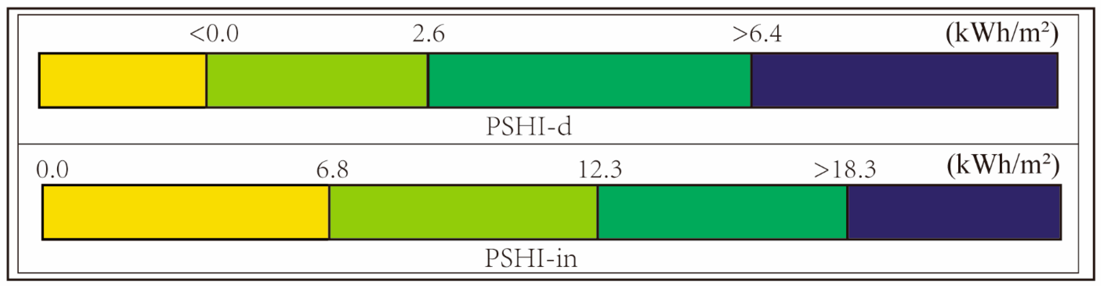
3.4. Indicator Grading Results

This study utilized K-means cluster analysis to evaluate the practical application of the PSHI by categorizing the passive heating potential across different climate regions. After implementing the PSHS-d, it was observed that some buildings showed negative energy savings, indicating a potential increase in heating energy consumption. To ensure the indicator’s practical relevance, instances of negative energy savings were excluded, thereby creating a separate category. The elbow rule was then applied to determine the optimal number of clusters within the filtered dataset. By examining the dataset characteristics and considering the practical implications of the PSHI, this study explored various grading schemes ranging from 2 to 10 clusters, monitoring changes in the within-cluster sum of squares (WSCC) metric.
According to the elbow rule, increasing the cluster count, k, generally decreases the sum of squares of errors (SSE) and improves the homogeneity of samples within clusters. When k is less than the true classification number of the dataset, increasing k significantly enhances the quality of clustering and markedly reduces SSE. However, once k reaches the actual classification number, the reduction in SSE slows and plateaus with further increases, thus identifying the dataset’s true cluster count through an ‘elbow’ pattern in the graph. For PSHI-d cluster analysis (as shown in Figure 9), increasing k from 3 to 4 led to a drop in WSCC values from 366 to 157 (a 57% reduction) and further to 98 (a 33% reduction), pinpointing k=3 as the elbow point. Consequently, the optimal cluster count for the PSHS-d was determined to be three, culminating in a total of four clusters including the negative energy savings category. Likewise, the identification of the elbow phenomenon at k = 4 for the PSHS-in’s cluster analysis indicated an optimal count of 4 clusters.
Cluster centers were then calculated to establish grading thresholds, classifying heating potential levels from “L1” to “L4,” from low to high (as shown in Figure 10). For the PSHS-d, clusters were defined with thresholds set at 0 (differentiating between energy-saving and non-energy-saving), 2.6, and 6.4, which indicate diminished heating energy savings. For the PSHS-in, the PSHI-in hierarchical thresholds were established at 6.8, 12.3, and 18.3, as depicted in the figure below. This methodology provides a systematic framework for quantitatively assessing and enhancing PSHSs.

3.5. Limitations and Prospects of This Study

This study offers valuable insights into the evaluation of PSHSs, but it also acknowledges certain methodological and interpretative limitations. Initially, our analysis was based primarily on theoretical model buildings, without incorporating field test data. While the simulation tool used provided detailed estimates of energy savings, the lack of real-world validation could potentially limit the applicability of our findings, since it can result in discrepancies between the simulated energy savings of PSHSs and the actual energy savings observed in real buildings. Obtaining field data that include information on actual architectural geometry design, envelopes, and occupant behavior would significantly enhance the accuracy of the simulation assessments of PSHSs’ energy-saving potential in buildings. Additionally, this study did not comprehensively examine the impact of various building design parameters on the potential for energy savings. Moreover, the polynomial model employed, which focuses on building energy savings, may not capture the full extent of potential savings achievable through PSHSs, especially in regions with high altitudes. These limitations underscore the need for future research directions, including the collection and analysis of field test data and a more detailed investigation into the influence of various design parameters on the benefits of passive heating.
The PSHI developed in this study introduces a new quantitative tool for assessing the energy-saving potential of PSHSs across various global climates. Moving forward, this work will assist architects and engineers in developing more precise passive heating solutions adapted to specific climatic conditions and provide data support for policymakers to encourage the adoption of efficient passive heating technologies. Future research will delve into combining the PSHI zoning results with urban characteristics to create implementation guidelines, optimizing passive heating system designs and enhancing global building energy efficiency toward sustainable development goals.

4. Conclusions

In this study, we successfully developed passive heating potential indicators (PSHIs) based on a polynomial regression model and employed the K-means clustering method to systematically grade these indicators. This approach facilitated the quantitative assessment and optimization of PSHSs. This study’s key findings and conclusions include the following:
  • An in-depth examination of the PSHS-d has uncovered critical temperature points where energy-saving effects vary under different climatic conditions. Notably, the relationship between building energy savings and average outdoor temperature follows a nonlinear parabolic distribution, peaking at an average outdoor temperature of approximately −0.6 °C.
  • We constructed a relational model to assess building energy-saving potentials, incorporating temperature and solar radiation intensity as variables. This model not only quantifies the impact of these environmental factors on passive heating’s energy efficiency but also serves as a precise guide for building design and energy efficiency improvements.
  • The proposed passive heating potential metrics extend across a broad temperature range, enabling the assessment of energy-saving potential in climates from extremely cold to mild. This expansion significantly broadens the applicability of passive heating technologies.
  • By integrating experimental data, we determined the optimal number of PSHI ratings and their thresholds. Employing the elbow rule allowed us to identify the optimal number of clusters, facilitating a scientific categorization of the global energy-saving potential of passive heating through cluster analysis.

Author Contributions

W.M.: conceptualization, methodology, software, validation, formal analysis, investigation, visualization, and writing—original draft. G.Z.: supervision, resources, and conceptualization. X.Y.: funding acquisition and conceptualization. Q.L.: methodology. B.J.D.: supervision, resources, and conceptualization. All authors have read and agreed to the published version of the manuscript.

Funding

This study is supported by the Science and Technology Bureau of Beilin District, Xi’an (Grant No. GX2339).

Data Availability Statement

The raw data supporting the conclusions of this article will be made available by the authors on request.

Acknowledgments

The authors thank the professors and students at the University of Kitakyushu for their generous help with the full paper, from investigation to the checking process.

Conflicts of Interest

Author Gaochuan Zhang was employed by the company Zhejiang Southeast Architectural Design Group Co., Ltd. The remaining authors declare that the research was conducted in the absence of any commercial or financial relationships that could be construed as a potential conflict of interest.

References

  1. Dean, B.; Dulac, J.; Petrichenko, K.; Graham, P. Global Status Report 2016: Towards Zero-Emission Efficient and Resilient Buildings; Global Alliance for Buildings and Construction (GABC): Paris, France, 2016. [Google Scholar]
  2. Akhmat, G.; Zaman, K.; Shukui, T.; Sajjad, F. Does energy consumption contribute to climate change? Evidence from major regions of the world. Renew. Sustain. Energy Rev. 2014, 36, 123–134. [Google Scholar] [CrossRef]
  3. Pérez-Lombard, L.; Ortiz, J.; Pout, C. A review on buildings energy consumption information. Energy Build. 2008, 40, 394–398. [Google Scholar] [CrossRef]
  4. Nejat, P.; Jomehzadeh, F.; Taheri, M.M.; Gohari, M.; Majid, M.Z.A. A global review of energy consumption, CO2 emissions and policy in the residential sector (with an overview of the top ten CO2 emitting countries). Renew. Sustain. Energy Rev. 2015, 43, 843–862. [Google Scholar] [CrossRef]
  5. Li, J.; Shan, M.; Baumgartner, J.; Carter, E.; Ezzati, M.; Yang, X. Laboratory study of pollutant emissions from wood charcoal combustion for indoor space heating in China. In Proceedings of the 13th International Conference on Indoor Air Quality and Climate, Indoor Air 2014, Hong Kong, China, 7–12 July 2014. [Google Scholar]
  6. Sobouti, H.; Alavi, P. Energy Management Strategy in Rural Housing (Case Study: Cold Climate). Middle-East J. Sci. Res. 2015, 23, 823–834. [Google Scholar]
  7. Alaeipour, M.S.; Mafi, M.; Khanaki, M.; Ebrahimi, M. Techno-economic feasibility of energy supply systems from renewable sources of solar and biomass in rural areas located in cold and dry climate. Amirkabir J. Mech. Eng. 2019, 53, 81–100. [Google Scholar]
  8. Kou, F.; Shi, S.; Zhu, N.; Song, Y.; Zou, Y.; Mo, J.; Wang, X. Improving the indoor thermal environment in lightweight buildings in winter by passive solar heating: An experimental study. Indoor Built Environ. 2022, 31, 2257–2273. [Google Scholar] [CrossRef]
  9. Li, J.; Cao, Y.; Wang, Q.; Niu, B. Potential of Solar Heating for Ultra-Low-Energy Passive Buildings in Cold Regions. Int. J. Heat Technol. 2019, 37, 1052–1058. [Google Scholar] [CrossRef]
  10. Li, L.; Chen, G.; Zhang, L.; Zhou, J. Research on the application of passive solar heating technology in new buildings in the Western Sichuan Plateau. Energy Rep. 2021, 7, 906–914. [Google Scholar] [CrossRef]
  11. Liu, Y.; Jiang, J.; Wang, D.; Liu, J. The passive solar heating technologies in rural school buildings in cold climates in China. J. Build. Phys. 2018, 41, 339–359. [Google Scholar] [CrossRef]
  12. Bataineh, K.M.; Fayez, N. Analysis of thermal performance of building attached sunspace. Energy Build. 2011, 43, 1863–1868. [Google Scholar] [CrossRef]
  13. Stevanović, S. Optimization of passive solar design strategies: A review. Renew. Sustain. Energy Rev. 2013, 25, 177–196. [Google Scholar] [CrossRef]
  14. Evins, R. A review of computational optimisation methods applied to sustainable building design. Renew. Sustain. Energy Rev. 2013, 22, 230–245. [Google Scholar] [CrossRef]
  15. Kheiri, F. A review on optimization methods applied in energy-efficient building geometry and envelope design. Renew. Sustain. Energy Rev. 2018, 92, 897–920. [Google Scholar] [CrossRef]
  16. Priya, R.S.; Sundarraja, M.; Radhakrishnan, S.; Vijayalakshmi, L. Solar passive techniques in the vernacular buildings of coastal regions in Nagapattinam, TamilNadu-India—A qualitative and quantitative analysis. Energy Build. 2012, 49, 50–61. [Google Scholar] [CrossRef]
  17. Lin, Y.; Zhao, L.; Liu, X.; Yang, W.; Hao, X.; Tian, L. Design Optimization of a Passive Building with Green Roof through Machine Learning and Group Intelligent Algorithm. Buildings 2021, 11, 192. [Google Scholar] [CrossRef]
  18. GB/T 37526-2019; Assessment Method for Solar Energy Resource. Standards Press of China: Beijing, China, 2019.
  19. JGJ/T 267-2012; Technical Code for Passive Solar Buildings. China’s Ministry of Housing and Urban-Rural Development, China Building Industry Press: Beijing, China, 2012.
  20. Meng, X.; Liu, Y.; Han, Y.; Cao, Q.; Zhang, S.; Yang, L. Defining and grading passive solar heating potential indicator in China: A new irradiation degree hour ratio parameter. Sol. Energy 2023, 252, 342–355. [Google Scholar] [CrossRef]
  21. Yang, L.; Zhu, X.; Liu, Y.; Liu, J. Review of design standard for energy efficiency of residential buildings in Tibet Autonomous Region. HV AC 2010, 40, 51–54. [Google Scholar]
  22. Joe, J.; Karava, P. A model predictive control strategy to optimize the performance of radiant floor heating and cooling systems in office buildings. Appl. Energy 2019, 245, 65–77. [Google Scholar] [CrossRef]
  23. Ghorbani, A.; Jahanpour, R.; Hasanzadehshooiili, H. Evaluation of liquefaction potential of marine sandy soil with piles considering nonlinear seismic soil–pile interaction; A simple predictive model. Mar. Georesources Geotechnol. 2020, 38, 1–22. [Google Scholar] [CrossRef]
  24. Gomes, G.J.C.; Gomes, R.G.D.S.; Vargas, E.D.A., Jr. A dual search-based EPR with self-adaptive offspring creation and compromise programming model selection. Eng. Comput. 2021, 38, 2155–2173. [Google Scholar] [CrossRef]
  25. Jin, Y.-F.; Yin, Z.-Y. An intelligent multi-objective EPR technique with multi-step model selection for correlations of soil properties. Acta Geotech. 2020, 15, 2053–2073. [Google Scholar] [CrossRef]
  26. Jin, Y.-F.; Yin, Z.-Y.; Zhou, W.-H.; Yin, J.-H.; Shao, J.-F. A single-objective EPR based model for creep index of soft clays considering L2 regularization. Eng. Geol. 2019, 248, 242–255. [Google Scholar] [CrossRef]
  27. Yin, Z.Y.; Jin, Y.F.; Yin, Z.Y.; Jin, Y.F. Optimization-Based Evolutionary Polynomial Regression. In Practice of Optimisation Theory in Geotechnical Engineering; Springer: Singapore, 2019. [Google Scholar] [CrossRef]
  28. Akhlaghi, Y.G.; Ma, X.; Zhao, X.; Shittu, S.; Li, J. A statistical model for dew point air cooler based on the multiple polynomial regression approach. Energy 2019, 181, 868–881. [Google Scholar] [CrossRef]
  29. Qian, X.; Lee, S.; Soto, A.-M.; Chen, G. Regression Model to Predict the Higher Heating Value of Poultry Waste from Proximate Analysis. Resources 2018, 7, 39. [Google Scholar] [CrossRef]
  30. Khoshkroudi, S.S.; Sefidkouhi, M.A.G.; Ahmadi, M.Z.; Ramezani, M. Prediction of soil saturated water content using evolutionary polynomial regression (EPR). Arch. Agron. Soil Sci. 2014, 60, 1155–1172. [Google Scholar] [CrossRef]
  31. Su, L.; Zhao, Y.; Yan, T.; Li, F. Local polynomial estimation of heteroscedasticity in a multivariate linear regression model and its applications in economics. PLoS ONE 2012, 7, e43719. [Google Scholar] [CrossRef] [PubMed]
  32. Kakoudakis, K.; Behzadian, K.; Farmani, R.; Butler, D. Pipeline failure prediction in water distribution networks using evolutionary polynomial regression combined with K-means clustering. Urban Water J. 2017, 14, 737–742. [Google Scholar] [CrossRef]
  33. Miao, D.; Wang, W.; Lv, Y.; Liu, L.; Yao, K.; Sui, X. Research on the classification and control of human factor characteristics of coal mine accidents based on K-Means clustering analysis. Int. J. Ind. Ergon. 2023, 97, 103481. [Google Scholar] [CrossRef]
  34. Li, C.; Sun, L.; Jia, J.; Cai, Y.; Wang, X. Risk assessment of water pollution sources based on an integrated k-means clustering and set pair analysis method in the region of Shiyan, China. Sci. Total. Environ. 2016, 557–558, 307–316. [Google Scholar] [CrossRef] [PubMed]
  35. Du, X.; Niu, D.; Chen, Y.; Wang, X.; Bi, Z. City classification for municipal solid waste prediction in mainland China based on K-means clustering. Waste Manag. 2022, 144, 445–453. [Google Scholar] [CrossRef]
  36. Zhang, S.; Wang, R.; Lin, Z. Subzone division optimization with probability analysis-based K-means clustering for coupled control of non-uniform thermal environments and individual thermal preferences. J. Affect. Disord. 2023, 249, 111155. [Google Scholar] [CrossRef]
  37. EnergyPlus. Available online: https://energyplus.net/weather (accessed on 6 October 2023).
  38. climate.onebuilding. Available online: https://climate.onebuilding.org/about/default.html (accessed on 16 March 2024).
  39. Synnefa, A.; Santamouris, M.; Akbari, H. Estimating the effect of using cool coatings on energy loads and thermal comfort in residential buildings in various climatic conditions. Energy Build. 2007, 39, 1167–1174. [Google Scholar] [CrossRef]
  40. Solgi, E.; Memarian, S.; Moud, G.N. Financial viability of PCMs in countries with low energy cost: A case study of different climates in Iran. Energy Build. 2018, 173, 128–137. [Google Scholar] [CrossRef]
  41. Premrov, M.; Leskovar, V.Ž.; Mihalič, K. Influence of the building shape on the energy performance of timber-glass buildings in different climatic conditions. Energy 2016, 108, 201–211. [Google Scholar] [CrossRef]
  42. Ahangari, M.; Maerefat, M. An innovative PCM system for thermal comfort improvement and energy demand reduction in building under different climate conditions. Sustain. Cities Soc. 2019, 44, 120–129. [Google Scholar] [CrossRef]
  43. Compagnon, R. Solar and daylight availability in the urban fabric. Energy Build. 2004, 36, 321–328. [Google Scholar] [CrossRef]
  44. Carletti, C.; Sciurpi, F.; Pierangioli, L. The Energy Upgrading of Existing Buildings: Window and Shading Device Typologies for Energy Efficiency Refurbishment. Sustainability 2014, 6, 5354–5377. [Google Scholar] [CrossRef]
  45. Strømann-Andersen, J.; Sattrup, P.A. The urban canyon and building energy use: Urban density versus daylight and passive solar gains. Energy Build. 2011, 43, 2011–2020. [Google Scholar] [CrossRef]
  46. Ménard, R.; Souviron, J. Passive solar heating through glazing: The limits and potential for climate change mitigation in the European building stock. Energy Build. 2020, 228, 110400. [Google Scholar] [CrossRef]
  47. Givoni, B. Comfort, climate analysis and building design guidelines. Energy Build. 1992, 18, 11–23. [Google Scholar] [CrossRef]
  48. Hu, Z.; Luo, B.; He, W. An Experimental Investigation of a Novel Trombe Wall with Venetian Blind Structure. Energy Procedia 2015, 70, 691–698. [Google Scholar] [CrossRef]
  49. Bojić, M.; Johannes, K.; Kuznik, F. Optimizing energy and environmental performance of passive Trombe wall. Energy Build. 2014, 70, 279–286. [Google Scholar] [CrossRef]
  50. He, W.; Hu, Z.; Luo, B.; Hong, X.; Sun, W.; Ji, J. The thermal behavior of Trombe wall system with venetian blind: An experimental and numerical study. Energy Build. 2015, 104, 395–404. [Google Scholar] [CrossRef]
Figure 1. Geographical distribution of studied cities across the global map.
Buildings 14 01364 g001
Figure 2. Model of simulated building.
Buildings 14 01364 g002
Figure 3. Simulation tools in experiment.
Buildings 14 01364 g003
Figure 4. Correlation between heating energy saving potential and environmental factors for PSHS-d and PSHS-in. (a) PSHI-d vs. Ta; (b) PSHI-d vs. Td; (c) PSHI-d vs. SRIt; (d) PSHI-d vs. SRIs;(e) PSHI-in vs. Ta; (f) PSHI-in vs. Td; (g) PSHI-in vs. SRIt; (h) PSHI-in vs. SRIs.
Buildings 14 01364 g004
Figure 5. Predictive regression models of solar heating efficiency using climatic variables.
Buildings 14 01364 g005
Figure 6. Global distribution of ITR, C-IDHR, PSHI-d, and PSHI-in.
Buildings 14 01364 g006
Figure 7. Comparative analysis of passive solar heating indicators, ITR, C-IDHR, and PSHI-d, in the context of climatic variables.
Buildings 14 01364 g007
Figure 8. Comparative analysis of passive solar heating indicators, ITR, C-IDHR, and PSHI-in, in the context of climatic variables.
Buildings 14 01364 g008
Figure 9. Variation in WSCC values with cluster count in PSHI-d and PSHI-in analyses. (a) PHSI-d; (b) PHSI-in.
Buildings 14 01364 g009
Figure 10. Threshold-based categorization of PSHI-d and PSHI-in using K-means clustering.
Buildings 14 01364 g010
Table 1. Thermal conductivity of building exterior envelope used in experiment.
Thermal ZoneComponent
Exterior WallExterior RoofExterior Window
11.473.760.18
22.174.640.22
32.354.640.25
42.885.520.32
53.235.520.32
63.585.520.34
73.586.400.43
84.816.400.50
Table 2. Set-points of building models used in experiment.
ParameterDescription
Internal heat gainLighting: 8 W/m2; equipment: 5 W/m2
People density30 m2/per people
Occupancy schedule24 h per day throughout the year
Temperature set-point for ideal air conditioningHeating: 18 °C
Air infiltrationAir flow per exterior surface area (m3/s·m2) = 0.00033
Table 3. Comparative regression models for PSHS-d and PSHS-in across 8 scenarios.
Predictive ModelR2MSE
Scenario 1 y = 4.96 + 0.16 T a + 0.22 S R I s 0.01 T a 2 0.01 T a S R I s 0.892.40
Scenario 2 y = 3.96 + 0.05 T d + 0.13 S R I s 0.01 T d 2 + 0.01 T d S R I s 0.872.40
Scenario 3 y = 2.25 + 0.17 T a + 0.06 S R I t 0.01 T d 2 0.666.16
Scenario 4 y = 1.96 + 0.04 T d + 0.03 S R I t 0.01 T d 2 0.567.99
Scenario 5 y = 9.08 0.51 T a + 0.03 S R I s 0.922.72
Scenario 6 y = 0.55 + 0.43 T d + 0.01 S R I s 0.912.86
Scenario 7 y = 9.00 0.51 T a 0.01 S R I t 0.912.74
Scenario 8 y = 0.38 + 0.45 T d 0.01 S R I t 0.922.74
Disclaimer/Publisher’s Note: The statements, opinions and data contained in all publications are solely those of the individual author(s) and contributor(s) and not of MDPI and/or the editor(s). MDPI and/or the editor(s) disclaim responsibility for any injury to people or property resulting from any ideas, methods, instructions or products referred to in the content.

