
Structural Optimization Study on a Three-Degree-of-Freedom Piezoelectric Ultrasonic Transducer

School of Physics and Electronic Science, Changsha University of Science and Technology, Changsha 410114, China
*
Author to whom correspondence should be addressed.
Actuators 2024, 13(5), 177; https://doi.org/10.3390/act13050177
Submission received: 31 March 2024
/
Revised: 29 April 2024
/
Accepted: 1 May 2024
/
Published: 8 May 2024
Abstract
:A three-degree-of-freedom (3-DOF) piezoelectric ultrasonic transducer is a critical component in elliptical and longitudinal ultrasonic vibration-assisted cutting processes, with its geometric structure directly influencing its performance. This paper proposes a structural optimization method based on a convolutional neural network (CNN) and non-dominated sorting genetic algorithm II (NSGA2). This method establishes a transducer lumped model to obtain the electromechanical coupling coefficients (X- and Z-) and thermal power (X-P) indicators, evaluating the bending and longitudinal vibration performance of the transducer. By creating a finite element model of the transducer with mechanical losses, a dataset of different transducer performance parameters, including the tail mass, piezoelectric stack, and dimensions of the horn, is obtained. Training a CNN model with this dataset yields objective functions for the relationship between different transducer geometric structures and performance parameters. The NSGA2 algorithm solves the X- and Z- objective functions, obtaining the Pareto set of the transducer geometric dimensions and determining the optimal transducer geometry in conjunction with X-P. This method achieves simultaneous improvements in X- and Z- of the transducer by 22.33% and 25.89% post-optimization and reduces X-P to 18.97 W. Furthermore, the finite element simulation experiments of the transducer validate the effectiveness of this method.
1. Introduction
A three-degree-of-freedom (3-DOF) piezoelectric transducers can generate elliptical ultrasonic vibration and longitudinal ultrasonic vibration independently and can be used to assist milling and drilling [1], respectively. By selecting appropriate elliptical [2,3,4,5,6] or longitudinal [7,8,9,10] vibration parameters, the cutting force and temperature in machining can be greatly reduced, and the surface quality of the workpiece can be improved. Therefore, it is an important component for assisting cutting. The structure [11,12] of the transducer consists of a tail mass and horn clamped by a hexagonal bolt and a piezoelectric ceramic stack for generating elliptical and longitudinal vibrations fixed in the middle. Therefore, the total energy [13,14] during operation includes the mechanical energy, loss, and electrical storage energy. The ratio of mechanical energy to total energy is called the electromechanical coupling coefficient [15]. The energy lost during vibration can be characterized by heat power [16,17,18]. In order to make the transducer have vibration kinetic energy and reduce loss during operation, a piezoelectric material with low loss and large [19] is selected. In addition, the geometric structure [16,20] of the transducer can be optimized to improve the electromechanical coupling coefficient and reduce the heat power.
The electromechanical coupling coefficient and heat power performance of elliptical and longitudinal vibration ultrasonic piezoelectric transducers are mainly studied in terms of the relationship between the geometric structure and optimization through theoretical modeling, finite element simulation, and experiments. Zhou et al. [19,20,21,22] established theoretical models, finite element models, and experimental studies of single longitudinal or flexural ultrasonic vibration to study the performance of the transducer, such as axial and flexural vibration modes, resonant frequency, electrical impedance characteristics, and frequency response characteristics. They provide evaluation criteria for transducer performance optimization. Zhang et al. [23] analyzed the influence of piezoelectric ceramic position on the resonant frequency and effective electromechanical coupling coefficient in theoretical models or experiments and optimized the electromechanical coupling coefficient performance under different cross-sectional lengths. Similarly, the literature [1] developed a longitudinal elliptical composite vibration ultrasonic transducer to realize the longitudinal and elliptical vibration ultrasonic-assisted machining functions. However, there is not much research on the optimal design of the electromechanical coupling coefficient performance of the transducer under multiple dimensional variations.
In addition, the elliptical or longitudinal vibration of the transducer will generate a large amount of heat due to internal friction [24], causing the temperature of the transducer to rise and be damaged. In order to reduce the heat power, Shi et al. analyzed and fitted the temperature rise curve of the heat power of piezoelectric ceramic wafers under the excitation of a shock wave electric field through experiments and analytical methods [25]. Some researchers have also established a nonlinear transmission matrix model of piezoelectric ceramics and a heat conduction equation and, combined with experiments, obtained the heat power and temperature rise results of piezoelectric devices resonating at high power [18]. Dong [26] et al. proposed a decoupled equivalent circuit to simulate piezoelectric discs in the radial vibration mode, considering three types of internal losses: dielectric loss, elastic loss, and piezoelectric loss. The experimental results show that the decoupling equivalent circuit has better accuracy than traditional circuits. The temperature rise caused by the non-resonant dielectric loss and resonant mechanical loss of a single piezoelectric ceramic was analyzed and experimentally studied [27]. Finally, it was concluded that the heat generation of the transducer at non-resonant and resonant frequencies was mainly caused by dielectric and mechanical heat generation, respectively, and it was found that the setting of the convection heat transfer coefficient between the transducer surface and the air seriously affected the temperature rise of the transducer. Furthermore, Vasiljev et al. [16] proposed a method to reduce the heat power of the transducer by separating the piezoelectric ceramic elements and adding metal blocks between the elements. However, they have not thoroughly investigated the thermal power performance of the transducer under multiple dimensional variations.
To the best of our knowledge, there is no detailed investigation on the comprehensive optimization of two electromechanical coupling coefficients of elliptical and longitudinal piezoelectric ceramics and on the analysis of thermal power performances when multiple geometric dimensions of a 3-DOF transducer varied. To address this issue, this paper explores a fast geometrical structure optimization method based on a multi-objective genetic algorithm by investigating the lumped-parameter model, finite element model, and neural network model of the 3-DOF piezoelectric transducer.
2. Geometry and Working Principle
A 3-DOF sandwich piezoelectric ultrasonic transducer is shown in Figure 1a. It consists of a hexagon bolt, a tail mass, piezoelectric ceramic stacks, a fixed fixture, a horn, and a tool. The hexagon bolt fixes the piezoelectric ceramic stack and fixed fixture by clamping the tail mass and the horn, preventing damage to the transducer during resonance. The tail mass is selected from a material with a larger impedance than the other parts. The size of the transducer decreases from the tail mass to the tool cross-sectional area so that the energy is concentrated on the tool. The function of the horn is to provide a larger output amplitude for the transducer tip. Piezoelectric ceramics with small loss and appropriate size are used to reduce the thermal energy generated during resonance that damages the transducer.
3-DOF transducer elliptical and longitudinal ultrasonic vibrations depend on the piezoelectric stack, which is divided into three groups from left to right: the X-direction, Y-direction, and Z-direction piezoceramic materials (in order to ensure that the displacement amplitude in the Z-direction is basically consistent with the magnitude range in the X-direction during vibration, the length of Z-PZT is slightly larger than that of in the X-direction and is simplified as X-, Y-, and Z-PZT), as shown in Figure 2d. X-PZT includes two piezoelectric ceramic rings (divided by the YZ plane to form two half-piezoelectric ceramic rings). The two half-sheets in its X-positive plane have opposite polarization directions, and the negative plane is the same, opposite to that in the positive plane. Y-PZT is consistent with X-PZT except for the direction, so only the X-direction needs to be considered when performing performance and lumped model analyses. Z-PZT only includes two piezoelectric ceramic rings with opposite polarization directions. Figure 2e shows the electrode connection method of the three groups of piezoelectric ceramic rings, and the copper electrodes with the same cross-sectional area as the piezoelectric ceramic rings provide an interface for the alternating current (AC) signal. the arrows represent the polarization directions of the four halves of X-PZT (similar to Y-PZT). When the piezoelectric ceramic stacks are excited by AC signals at their resonant frequencies, the transducer produces X-, Y-, and Z-direction resonances, respectively. Among them, when the X- and Y-directions resonate together, the tool tip generates an elliptical trajectory, which is called elliptical ultrasonic-assisted vibration milling. The Z-direction is used for drilling alone. After being amplified by the horn and reflected by the tail mass, a large displacement amplitude is generated at the tool tip. The entire transducer fixture is actually fixed in the tool holder, and the piezoelectric ceramic ring is powered by a carbon brush, which works on a high-speed rotating milling or drilling machine tool, machining the workpiece more effectively.
In this paper, the high-speed rotation state of the transducer and the contact between the tool and the workpiece mainly affect the stability performance of the displacement amplitude during the operation of the transducer. Its stability can be improved through the transducer control algorithm, so it will not be studied. Only the geometric optimization problem is considered, so the material properties of the piezoelectric stack and other metal parts of the transducer remain unchanged, as shown in Tables 2 and 3. In addition, considering the geometric structure limitations of 3-DOF transducer in milling and drilling, the approximate geometric dimensions [1] of a 3-DOF transducer can be obtained as shown in Table 1.
2.1. Working Principle
In order to better meet the requirements of auxiliary milling and drilling functions, this paper obtains the evaluation parameters of transducer performance by studying the control equation of piezoelectric materials and the lumped model of transducers. The purpose is to prepare for further geometric optimization designing of the transducer.
2.1.1. Piezoelectric Constitutive Equations
Piezoelectric ceramic rings are the core components of the transducer. Their control equation is the piezoelectric inverse effect. By applying a periodic AC signal to the polarized piezoelectric ceramic, it generates mechanical vibration, which in turn drives the transducer tip to generate periodic output displacement. The d-type piezoelectric equations [17] are shown in Equations (1) and (2).
where S, T, D, and E represent the strain, stress, electric displacement, and electric field strength matrix, respectively. d, , and represent the 3 × 6 coupling coefficient matrix, the 3 × 3 dielectric constant matrix, and the 6 × 6 compliance coefficient matrix, respectively. Their values are all temperature-dependent and are related to the characteristics of the material. There is symmetry in the values in the piezoelectric ceramic coefficient matrix, and a large number of the coefficients are zero. Due to the use of bolt-clamped piezoelectric rings in this study and the relatively low excitation voltage, only their linear behavior is considered. The expanded equations can thus be written as in Equations (3)–(11).
where the subscripts of constants and variables correspond to their positions in the matrix. In finite element software, only the values of the coefficient matrix need to be set.
2.1.2. Lumped Model
The simplified mechanical model of the piezoelectric transducer is equivalent to the lumped circuit model, which is further simplified to the electromechanical equivalent circuit to obtain its performance parameters, as shown in Figure 2. In the mechanical lumped model of the transducer, the tail mass and part of the bolt of the piezoelectric transducer are simplified to the tail mass, and only the X- and Z-PZT are considered in the piezoelectric stack. The fixture, horn, and tool are simplified to the front mass, as shown in Figure 2a. The circuit elements and mechanical concentrated model components in the simplified equivalent circuit model correspond one-to-one, as shown in Figure 2b. The final simplified electromechanical equivalent circuit includes four circuit elements, as shown in Figure 2c. The performance parameters of the transducer can be obtained from the electromechanical equivalent circuit, such as Equations (12) and (13) [23].
where Z, V, and I are the impedance, excitation voltage, and excitation current of the transducer in each axial direction, respectively. , , and represent the electromechanical coupling coefficient, static, and dynamic capacitance of the transducer (X- and Z- represent the electromechanical coupling coefficients of X-, and Z-PZT, respectively. Y- and X- are basically the same and are not considered). and are the series resonant frequency and parallel resonant frequency of the transducer, respectively.
The dynamic resistance R in the electromechanical equivalent circuit of the transducer is equivalent to damping in mechanical vibration. When the piezoelectric ceramic plate is excited by an AC signal and undergoes resonance, the vibration causes frictional motion between the molecules in the piezoelectric stack, resulting in the generation of heat energy due to loss. The loss can be characterized by establishing complex physical constants in the control equation. In this study, the piezoelectric ceramic uses materials with low loss, so its loss can be regarded as a disturbance, mainly including mechanical and dielectric losses. Therefore, the mechanical and dielectric loss coefficients [28,29] can be represented by Equations (14) and (15).
where represents the phase delay between the electrical displacement under constant stress and the applied electric field, and represents the phase lag between the strain under a constant electric field and the applied stress. Its value can be individually set in finite element software. In addition, the heat power generated [17] by the entire volume of the piezoelectric ceramic ring can be calculated using Equation (16).
where represents the peak voltage applied to the piezoelectric ceramic ring assembly and represents the real part of the admittance of the piezoelectric ceramic ring assembly (where X- and Z-P represent the heat power of X- and Z-PZT. Y-P and X-P are essentially the same and are not considered. Additionally, the sum of X-, and Y-P is much larger than Z-P; hence, this study only considers X-P).
From the above, we can obtain the performance index parameters of the transducer: the effective electromechanical coupling coefficient and the transducer’s heat power P. The can reflect the efficiency of the transducer in converting electrical energy into mechanical energy, while P can intuitively indicate the amount of loss in the transducer. By evaluating the curie temperature of the piezoelectric material, the operational safety of the transducer can be determined.
3. Finite Element Model of the Transducer
The finite element model’s dimensions of the 3-DOF piezoelectric transducer in reference [1] are consistent with those in Table 1. Three sets of piezoelectric materials are PZT-8. the material of the horn, tail mass, and bolt are 304 steel, and the material of the remaining cutting tools is carbidet. The piezoelectric ceramics in the X- and Y-directions consist of two sets of two half-rings, each with opposite polarity. The natural frequencies of the transducer in the X-, Y-, and Z-directions are 17.5 kHz, 17.4 kHz, and 16.6 kHz. By establishing a consistent finite element model of the transducer as presented in reference [1] and fitting the mechanical loss parameters, different finite element models with mechanical loss parameters were created for various geometric structures to obtain a dataset of performance parameters.
3.1. Fitting of Mechanical Loss Parameters
The loss of piezoelectric materials and the physical properties of the various parts of the transducer, as well as the geometric structures and external conditions, are closely related and have an extremely important impact on the performance parameters of the transducer, such as output amplitude and heat power. The characterization of piezoelectric material loss includes three types: mechanical, electromechanical coupling, and dielectric losses. The mechanical loss of the metal in the transducer at high frequencies can be ignored [13]. The dielectric losses of X-(Y-) and Z-PZT can be obtained from the literature [25] as 0.01 and 0.0125, respectively. The method for determining the mechanical loss parameters is as follows.
A finite element model of the 3-DOF piezoelectric transducer as described in reference [1] was established. The geometric parameters and material properties are shown in Table 1, Table 2 and Table 3. The horn adopts a hyperbolic shape, and its cross-sectional curve formula is given by Equation (17).
where , and represent the cross-sectional radius of the horn, the radius of the larger end cross-section of the horn, and the radius of the smaller end cross-section of the horn, respectively. Also, s represents the axial position of the horn cross-section, and it has a range of 0–5 mm. (s = 0) and (s = 5), respectively, represent the values of the radius of the larger end cross-section and the smaller end cross-section of the horn.
The hexagon bolt was imported from the COMSOL Multiphysics official website. The contact surfaces between the bolt head and the tail mass and between the bolt and the horn were set to uniform contact. The effect of friction was ignored, and a warning cutoff was employed. The pre-tightening force of the bolt was 3100 N, and a 50 mm length of the tool protruded by 35 mm, as shown in Figure 3 and Figure A1. Two cross-sections of the fixture ring were fixedly constrained. Regarding the polarization of the piezoelectric ceramic ring and the electrical circuit connection, X, Y, and Z-PZT groups were excited by an alternating signal voltage with a peak of 100 V and zero phase, as shown in Figure 2d,e. The physical fields considered were solid mechanics and static electric fields. The domain and coordinates were selected according to the polarization direction of the piezoelectric materials. The minimum mesh division of the finite element model for acoustic was determined using the empirical formula shown in Equation (18).
where the maximum frequency was set to = 25 kHz and the minimum speed of sound for the transducer material was = 3122 m/s, which resulted in a minimum grid value of n = 20.8 mm.The finite element model of the transducer in this study used a conventional tetrahedral mesh, with a maximum element size of 15.1 mm, which met the requirements of the mesh. The total number of elements in the mesh was 105,694. The piezoelectric ceramic mechanical loss was set to isotropic loss, with a parameter scanning range of 0.006 to 0.013 and a step size of 0.001. Frequency domain studies were conducted in a frequency range of 10–25 kHz with a step size of 5 Hz.
Finite element calculations were performed to obtain the displacement amplitude of the transducer’s tool tip () and impedance magnitude on logarithmic scale () curves as a function of frequency. The displacement amplitudes in the X- and Z-directions were denoted as X- and Z-, respectively. the impedance modulus of X- and Z-PZT were denoted as X- and Z-, as shown in Figure 4. The resonant frequencies in the X- and Z-directions were found to be 16.5 kHz and 17.8 kHz, respectively, with peak amplitudes ranging from approximately 8 to 17 μm. The X- and Z- displacements decreased with increasing damping, as shown in Figure 4a. The series resonance frequencies in the X- and Z-directions were 16.5 kHz and 17.8 kHz, and the parallel resonance frequencies were 17.05 kHz and 18.2 kHz. The peak values of X- and Z- were approximately ranging from 4.65 to 4.9 and from 4.25 to 4.55, respectively. The red and blue curves represent the X- and Z- curves from reference [1], and the frequencies of the model associated with the X-direction were 420 Hz higher than those reported in the literature, which is within the allowable error range. This discrepancy was considered by increasing the frequency values for the X-direction by 420 Hz for better comparison. The values of the Z-direction decreased first and then increased at 18.1 kHz. This was due to the influence of the Y-direction resonance mode on the actual 3-DOF transducer, which resulted in a decrease in the output amplitude of the X-direction at the resonance point, as shown in Figure 4b.
The peak values of X- and Z- displacements were approximately 10 μm and 12.5 μm in reference [1]. Meanwhile, in this study, when the mechanical losses were set to 0.009 and 0.01, the X- and Z-displacement values were 11.68 μm and 10.54 μm and 11.57 μm, 10.39 μm, respectively. After comprehensive considerations, the mechanical loss of the piezoelectric ceramic was chosen as 0.0095 in this study.
3.2. Finite Element Model of Geometric Variations
Based on the finite element model of mechanical parameter fitting, finite element models of transducers with different geometric structures were established by changing the geometric dimensions of the tail mass, X-PZT, and horn. The geometric dimensions of the transducer were varied as follows: The length and diameter of the tail mass varied in the ranges of 16–28 mm and 30–42 mm, respectively, with a step size of 4 mm for both. The length and diameter of the horn varied in the ranges of 20–35 mm and 17–29 mm, with step sizes of 5 mm and 4 mm, respectively. The lengths of the X (Y)-PZT varied in the range of 3.5–5.5 mm with a step size of 1 mm, while the length of the Z-PZT varied with the X-PZT, with an additional 0.5 mm. The geometric parameters were scanned as a whole. A total of 768 finite element models were created for the geometric variations. The pre-tightening bolts and tool dimensions remained fixed, while the geometric variations of the fixed clamps and nuts changed with other components, as shown in Figure 3. In evaluating the effect on transducer performance, the transducer piezoelectric stack material used was PZT-8, and the rest was 304 steel. In addition to geometric variations, the remaining software settings for different transducer finite element models were consistent with the model in the mechanical damping fitting, and the piezoelectric stack loss parameters were all set to 0.0095.
3.3. Simulation Calculation and Results
In this study, finite element simulations were performed using a computer with the following specifications: Windows 10 Professional 64-bit operating system, Intel(R) Core(TM) i5-8600K CPU @ 3.60GHz 3.60 GHz processor, and 64.0 GB RAM (63.8 GB available). We performed frequency domain computational studies on 768 different structural finite element transducer models. After excluding models with anomalous results, we obtained X-, Z-, and X-P data for 702 distinct transducer structures, as depicted in Figure 5.
Here, X- and Z- represent the electromechanical coupling coefficients in the X- and Z-directions, respectively, for the 3-DOF piezoelectric transducer. Because Z- is of the first order, overall, the value of Z- is greater than that of X-. The Z- values are below 40% and the X- values are below 30%, as shown in Figure 5a. X-P represents the heat power generated by the X-PZT during the bending vibration in the X-direction for the 3-DOF piezoelectric transducer. In all models, the X-P values are below 50W, as shown in Figure 5b.
4. Geometric Structure Optimization Method
The finite element model is used as the objective function model for the NSGA2 [32] algorithm. However, the computational time required is excessively long. Therefore, a dataset of performance indicators for different geometric structures of transducers is obtained through finite element model calculations. This dataset is then processed by a CNN [33] algorithm to obtain two objective functions, X- and Z-, which serve as the optimization objectives for the NSGA2 algorithm to solve for the Pareto optimal solution set of geometric dimensions for transducers.
4.1. Indicator Parameter CNN Model
Based on the analysis of the finite element models, from the 702 computed results of X-, Z-, and X-P, 600 were randomly selected as the training set for the CNN, with the remaining 102 being used as the test set. The CNN model took the input of five parameters: the tail mass length and diameter, X-PZT length, and horn length and diameter. The outputs were X-, Z-, and X-P.
The structure of the CNN model comprised 20 layers: the first layer had a 5 × 1 × 1 image input, followed by layers 2–4, which included 5 × 1 × 16 convolution, batch normalization, and ReLU layers. Layers 6–8 consisted of 4 × 1 × 32 max-pooling, convolution, batch normalization, and ReLU layers, and layers 9–12 included 3 × 1 × 64 max-pooling, convolution, batch normalization, and ReLU layers. Layers 13–16 utilized 2 × 1 × 128 max-pooling, convolution, batch normalization, and ReLU layers, layer 17 had 1 × 1 × 128 max-pooling, layer 18 was a dropout layer of 1 × 1 × 128, layer 19 was a fully connected layer of 1 × 1 × 1, and the final layer was the regression output layer.
The CNN model used the stochastic gradient descent method (SGDM) as the gradient descent algorithm, with a batch size of 300, maximum training count of 1200, and initial learning rate of 0.01 (which was decreased to 0.001 after 800 iterations). The training dataset was shuffled before each training session. The results of the CNN model on the test set are shown in Figure 6, where the root mean square error (RMSE) for X-, Z-, and X-P were found to be 0.858, 0.5136, and 2.116, respectively, indicating a high degree of fitting.
4.2. Based on NSHA2 Geometric Structure Optimization
The CNN network model for X- and Y- were obtained above as the two objective functions of NSGA2. There is no feasible solution that simultaneously achieves the optimal geometric parameters for the transducer. Therefore, the transducer geometric structure optimization design consists of two steps: (1) using the effective electromechanical coupling coefficients of the transducer’s X-PZT and Z-PZT as the objective functions, obtaining the Pareto optimal solution set of the transducer based on NSGA2; and (2) combining the transducer design requirements to subjectively make decisions on the Pareto optimal solution set, selecting the best solution closest to the optimal level (simultaneously optimal for both objectives).
4.2.1. Optimization of Two Targets
The five objective variables for optimizing the geometric structure of transducers in this study are as follows: the length () and diameter () of the tail mass, the length () of the X-PZT, and the length () and diameter () of the horn. The optimization objectives are X- and Y-.
where N represents a natural number. The NSGA2 algorithm is used to optimize these two objective functions, with an initial population size of 50 and 500 iterations. The cross-over and mutation probabilities are set at 0.8 and 0.05, respectively. The optimization process is shown in Figure 7.
4.2.2. Dual-Objective Optimization Decision
The results of the NSGA2 algorithm optimization are shown in Figure 8. The red region represents the Pareto solutions for the transducer X- and Z- at their optimal values simultaneously. The table presents seven solutions, as shown in Table 4, where X--Ture, Z--Ture, and X-P-Ture, respectively, indicate the true values obtained from the finite element simulation; X--Predict, Z--Predict, and X-P-Predict, respectively, represent the predicted values from the CNN with a maximum error not exceeding 3.63%. This indicates that the objective functions of X- and Z- obtained by the CNN fitting are effective. Moreover, the 3-DOF ultrasonic vibration transducer needs to operate near its resonance frequency to achieve high-frequency, high-amplitude vibration for the tool. However, high-frequency, high-amplitude vibration can increase the temperature of the transducer, leading to potential damage. Therefore, the solutions with high thermal power were excluded from the seven optimal solutions, resulting in the optimal geometric structure for the transducer as (22, 40, 5.5, 20, 23). The overall scheme of the geometric optimization of the transducer is presented in Figure 1.
5. Finite Element Verification
This paper utilized the finite element method to establish 15 finite element transducer models beyond the dataset and obtained the third-order X- indicator parameter for the transducer’s X-directional bending vibration and the first-order Z- indicator parameter for the longitudinal vibration to verify the correctness of the optimization method.
5.1. Geometric Variation
The obtained performance parameters were compared and validated with the optimal geometric structure transducer by singlehandedly varying the diameter and length of the tail mass, length of X-PZT, and diameter and length of the horn. The results are as follows.
5.1.1. Tail Mass Variation
The tail mass in the transducer not only serves to clamp and fix the piezoelectric ceramic, preventing its resonance destruction, but also reflects the ultrasonic energy to the cutting tool. Its geometric dimensions have a significant impact on the transducer’s performance. The diameter and length of the tail mass range from 18 to 26 mm and from 38 to 42 mm, with step lengths of 4 mm and 2 mm, respectively.
When the length of the tail mass is increased, the frequency range of interest is 16–21 kHz. The transducer’s resistance frequency (X- and Z-) and heat power frequency (X- and Z-P) curves are shown in Figure 9. The peak value of resistance corresponds to the series resonance frequency , while the peak value of power corresponds to the parallel resonance frequency . Using the obtained and , the corresponding values for different lengths of the tail mass of the transducer are calculated using Equation (13) and are presented in Table 5. The performance (X-, Z-, and X-P) of the transducer with the structure (22, 40, 5.5, 20, 23), as indicated in the table, is superior to the parameters before optimization.
When the diameter of the tail mass of the transducer is increased, the frequency range of concern is 16.5–20.5 kHz. The obtained X-, Z-, X-P, and Z-P curves are shown in Figure 10. Table 6 shows the corresponding series resonance frequency, parallel resonance frequency, thermal power value, and calculated electromechanical coupling coefficient of the transducer. The performance (X-, Z-, and X-P) of the transducer with the structure (22, 40, 5.5, 20, 23), as indicated in the table, is superior to the parameters before optimization.
5.1.2. X-PZT Variation
X-PZT (Y-PZT, besides causing the transducer to bend in the Y-direction, has the same structure and basic performance as X-PZT; no additional introduction is provided) is excited by an AC signal, causing the transducer to generate bending vibration in the X-direction through the inverse piezoelectric effect. During milling, together with the bending vibration of Y-PZT, it forms an ellipse, reducing milling force and temperature.
The length range of X-PZT is 3.5–5.5 mm. When the length of the X-PZT of the transducer is increased, the frequency range of concern is 16–21 kHz. The obtained X-, Z-, X-P, and Z-P curves are shown in Figure 11. Table 7 shows the corresponding series resonance frequency, parallel resonance frequency, thermal power value, and calculated electromechanical coupling coefficient of the transducer. The performance (X-, Z-, and X-P) of the transducer with the structure (22, 40, 5.5, 20, 23), as indicated in the table, is superior to the parameters before optimization.
5.1.3. Horn Variation
The horn in the transducer plays a role in amplifying the displacement amplitude while also needing to possess strong rigidity to ensure that the tool does not damage the workpiece upon contact. The length and diameter of the horn vary within the ranges of 20–28 mm and 23–27 mm, respectively, with a step of 4 mm for both.
When the length of the horn of the transducer is increased, the frequency range of concern is 16–21 kHz. The obtained X-, Z-, X-P, and Z-P curves are shown in Figure 12. Table 8 shows the corresponding series resonance frequency, parallel resonance frequency, thermal power value, and calculated electromechanical coupling coefficient of the transducer. The performance (X-, Z-, and X-P) of the transducer with the structure (22, 40, 5.5, 20, 23), as indicated in the table, is superior to the parameters before optimization.
When the diameter of the horn of the transducer is increased, the frequency range of concern is 15.5–20.5 kHz. The obtained X-, Z-, X-P, and Z-P curves are shown in Figure 13. Table 9 shows the corresponding series resonance frequency, parallel resonance frequency, thermal power value, and calculated electromechanical coupling coefficient of the transducer. The performance (X-, Z-, and X-P) of the transducer with the structure (22, 40, 5.5, 20, 23), as indicated in the table, is superior to the parameters before optimization.
5.2. Optimized Transducer Structure
6. Conclusions
This paper proposes a geometric structure optimization method for a 3-DOF transducer. By studying the transducer’s concentrated model, the evaluation parameters and P, which assess the transducer’s performance, were obtained. Different transducer finite element models with a mechanical loss value of 0.0095 were established to obtain the dataset of indicator parameter values in the X- and Z-directions. Two objective functions were obtained using CNN to establish the relationship between the transducer’s geometric dimensions and indicator parameters, with RMSE values of 0.858, 0.5136, and 2.116 for the X-, Z-, and X-P test sets and actual values, respectively. Taking X- and Z- as the objective function of NSGA2, the Pareto optimal solution set was obtained, and the optimized geometric structure of the transducer was determined to be (22, 40, 5.5, 20, 23) through subjective decision making. Finally, by establishing a finite element model of the transducer using data beyond the dataset, the optimized transducer’s X- and Z-PZT electromechanical coupling coefficients can simultaneously reach 22.33% and 25.89%, respectively, with the thermal power of X-PZT being reduced to 18.97 W. This is a 2.4% and 1.87% increase in the effective electromechanical coupling coefficients of X- and Z-PZT, respectively, compared with the model in the literature, with X-PZT’s thermal power being reduced by 1.33 W. This indicates that the method presented in this paper has achieved the optimal geometric structure for the transducer.
Author Contributions
Conceptualization, F.H.; data curation, C.G.; investigation, D.W.; resources, Y.C.; software, Z.Z.; visualization, L.T.; writing—original draft, Z.W. All authors have read and agreed to the published version of the manuscript.
Funding
This work was supported by the Scientific Research Fund of Hunan Provincial Education Department CX20220960.
Institutional Review Board Statement
Not applicable.
Informed Consent Statement
Not applicable.
Data Availability Statement
Data are contained within the article.
Conflicts of Interest
The funders had no role in the design of the study. The authors declare that they have no known competing financial interests or personal relationships that could have appeared to influence the work reported in this paper.
Appendix A
To illustrate the relevant details of the finite element model of the transducer, the side view of the model is shown in Figure A1.
Figure A1.
Side view of transducer model.

References
- Gao, J.; Altintas, Y. Development of a three-degree-of-freedom ultrasonic vibration tool holder for milling and drilling. IEEE ASME Trans. Mechatron. 2019, 24, 1238–1247. [Google Scholar] [CrossRef]
- Han, X.; Zhang, D. Effects of separating characteristics in ultrasonic elliptical vibration-assisted milling on cutting force, chip, and surface morphologies. Int. J. Adv. Manuf. Technol. 2020, 108, 3075–3084. [Google Scholar] [CrossRef]
- Zhang, M.; Zhang, D.; Geng, D.; Shao, Z.; Liu, Y.; Jiang, X. Effects of tool vibration on surface integrity in rotary ultrasonic elliptical end milling of Ti–6Al–4V. J. Alloys Compd. 2020, 821, 153266. [Google Scholar] [CrossRef]
- Liu, J.; Jiang, X.; Han, X.; Zhang, D. Influence of parameter matching on performance of high-speed rotary ultrasonic elliptical vibration-assisted machining for side milling of titanium alloys. Int. J. Adv. Manuf. Technol. 2019, 101, 1333–1348. [Google Scholar] [CrossRef]
- Zhang, M.; Zhang, D.; Geng, D.; Liu, J.; Shao, Z.; Jiang, X. Surface and sub-surface analysis of rotary ultrasonic elliptical end milling of Ti-6Al-4V. Mater. Des. 2020, 191, 108658. [Google Scholar] [CrossRef]
- Du, P.; Han, L.; Qiu, X.; Chen, W.; Deng, J.; Liu, Y.; Zhang, J. Development of a high-precision piezoelectric ultrasonic milling tool using longitudinal-bending hybrid transducer. Int. J. Mech. Sci. 2022, 222, 107239. [Google Scholar] [CrossRef]
- Liu, Q.; Xu, J.; Yu, H. Experimental study of tool wear and its effects on cutting process of ultrason-ic-assisted milling of Ti6Al4V. Int. J. Adv. Manuf. Technol. 2020, 108, 2917–2928. [Google Scholar] [CrossRef]
- Jing, L.; Niu, Q.; Yue, W.; Rong, J.; Gao, H.; Tang, S. Groove bottom material removal mechanism and machinability evaluation for longitudinal ultrasonic vibration–assisted milling of Al-50wt% Si alloy. Int. J. Adv. Manuf. Technol. 2023, 127, 365–380. [Google Scholar] [CrossRef]
- Xie, W.; Wang, X.; Liu, E.; Wang, J.; Tang, X.; Li, G.; Zhang, J.; Yang, L.; Chai, Y.; Zhao, B. Research on cutting force and surface integrity of TC18 titanium alloy by longitudinal ultrasonic vibration assisted milling. Int. J. Adv. Manuf. Technol. 2022, 119, 4745–4755. [Google Scholar] [CrossRef]
- Su, Y.; Li, L. Surface integrity of ultrasonic-assisted dry milling of SLM Ti6Al4V using polycrystalline diamond tool. Int. J. Adv. Manuf. Technol. 2022, 119, 5947–5956. [Google Scholar] [CrossRef]
- Zhang, J.-G.; Long, Z.-L.; Ma, W.-J.; Hu, G.-H.; Li, Y.-M. Electromechanical Dynamics Model of Ultrasonic Transducer in Ul-trasonic Machining Based on Equivalent Circuit Approach. Sensors 2019, 19, 1405. [Google Scholar] [CrossRef]
- Satpute, V.; Huo, D.; Hedley, J.; Elgendy, M. Design of a novel 2D ultrasonic transducer for 2D high-frequency vibration–assisted micro-machining. Int. J. Adv. Manuf. Technol. 2023, 126, 1035–1053. [Google Scholar] [CrossRef]
- Abdullah, A.; Malaki, M. On the damping of ultrasonic transducers’ components. Aerosp. Sci. Technol. 2013, 28, 31–39. [Google Scholar] [CrossRef]
- Shekhani, H.N.; Uchino, K. Characterization of mechanical loss in piezoelectric materials using tem-perature and vibration measurements. J. Amer. Ceram. Soc. 2014, 97, 2810–2814. [Google Scholar] [CrossRef]
- Wang, P.; Liu, J.; Chen, W.; Zhang, Q. Study on electromechanical coupling model of piezoelectric ultrasonic transducer. In Proceedings of the IEEE International Conference on Mechatronics & Automation, Takamatsu, Japan, 4–7 August 2013; IEEE: Piscataway, NJ, USA, 2013. [Google Scholar] [CrossRef]
- Vasiljev, P.; Mazeika, D.; Borodinas, S. Minimizing heat generation in a piezoelectric Langevin transducer. In Proceedings of the 2012 IEEE International Ultrasonics Symposium, Dresden, Germany, 7–10 October 2012; pp. 2714–2717. [Google Scholar] [CrossRef]
- Visvanathan, K. Bulk Micromachined Piezoelectric Transducers for Ultrasonic Heating of Biological Tissues. Dissertations & Theses—Gradworks. 2011. Available online: https://deepblue.lib.umich.edu/handle/2027.42/86544 (accessed on 12 April 2024).
- Miyake, S.; Ozaki, R.; Hosaka, H.; Morita, T. High-power piezoelectric vibration model considering the interaction between nonlinear vibration and temperature increase. Ultrasonics 2019, 93, 93–101. [Google Scholar] [CrossRef]
- Wang, L.; Hofmann, V.; Bai, F.; Jin, J.; Liu, Y.; Twiefel, J. Systematic electromechanical transfer matrix model of a novel sand-wiched type flexural piezoelectric transducer. Int. J. Mech. Sci. 2018, 138, 229–243. [Google Scholar] [CrossRef]
- Lin, S. Study on the Langevin piezoelectric ceramic ultrasonic transducer of longitudinal–flexural compo-site vibrational mode. Ultrasonics 2006, 44, 109–114. [Google Scholar] [CrossRef]
- Zhou, G.P. The performance and design of ultrasonic vibration system for flexural mode. Ultrasonics 2000, 38, 979–984. [Google Scholar] [CrossRef] [PubMed]
- Zhou, G.P.; Zhang, Y.H.; Zhang, B.F. The complex-mode vibration of ultrasonic vibration systems. Ultrasonics 2002, 40, 907–911. [Google Scholar] [CrossRef]
- Zhang, Q.; Shi, S.; Chen, W. An electromechanical coupling model of a longitudinal vibration type piezoe-lectric ultrasonic transducer. Ceram. Int. 2015, 41, S638–S644. [Google Scholar] [CrossRef]
- Uchino, K.; Zheng, J.H.; Chen, Y.H.; Du, X.H.; Ryu, J.; Gao, Y.; Ural, S.; Priya, S.; Hirose, S. Loss mechanisms and high power piezoelectrics. In Frontiers of Ferroelectricity; Springer: Boston, MA, USA, 2006. [Google Scholar] [CrossRef]
- Shi, H.; Chen, Z.; Chen, X.; Liu, S.; Cao, W. Self-heating phenomenon of piezoelectric elements excited by a tone-burst electric field. Ultrasonics 2021, 117, 106562. [Google Scholar] [CrossRef] [PubMed]
- Dong, X.; Uchino, K.; Jiang, C.; Jin, L.; Xu, Z.; Yuan, Y. Electromechanical Equivalent Circuit Model of a Piezoelectric Disk Considering Three Internal Losses. IEEE Access 2020, 8, 181848–181854. [Google Scholar] [CrossRef]
- Stewart, M.; Cain, M.G. Measurement and Modelling of Self-Heating in Piezoelectric Materials and Devices; Springer Series in Measurement Science and Technology; Springer: Dordrecht, The Netherlands, 2014; Volume 2. [Google Scholar] [CrossRef]
- Algueró, M.; Alemany, C.; Pardo, L.; González, A.M. Method for obtaining the full set of linear electric, mechanical, and electromechanical coefficients and all related losses of a piezoelectric ceramic. J. Am. Ceram. Soc. 2004, 87, 209. [Google Scholar] [CrossRef]
- Uchino, K.; Hirose, S. Loss mechanisms in piezoelectrics: How to measure different losses separately. IEEE Trans. Ultrason. Ferroelectr. Freq. Control 2001, 48, 307–321. [Google Scholar] [CrossRef] [PubMed]
- Mattiat, O.E.; Mason, W.P. Ultrasonic Transducer Materials. Phys. Today 1972, 25, 57–58. [Google Scholar] [CrossRef]
- Wu, Q.; Xie, D.-J.; Si, Y.; Zhang, Y.-D.; Li, L.; Zhao, Y.-X. Simulation analysis and experimental study of milling surface residual stress of Ti-10V-2Fe-3Al. J. Manuf. Process. 2018, 32, 530–537. [Google Scholar] [CrossRef]
- Deb, K.; Agrawal, S.; Pratap, A.; Meyarivan, T. A Fast Elitist Non-dominated Sorting Genetic Algorithm for Multi-objective Optimization: NSGA-II. In Parallel Problem Solving from Nature PPSN VI. PPSN 2000; Schoenauer, M., Deb, K., Rudolph, G., Yao, X., Lutton, E., Merelo, J.J., Schwefell, H.-P., Eds.; Lecture Notes in Computer Science; Springer: Berlin/Heidelberg, Germany, 2000; Volume 1917. [Google Scholar] [CrossRef]
- Fukushima, K. Neocognitron: A self-organizing neural network model for a mechanism of pattern recogni-tion unaffected by shift in position. Biol. Cybern. 1980, 36, 193–202. [Google Scholar] [CrossRef]
Figure 1.
Workflow diagram of the proposed methodology: (a) 3-DOF piezoelectric ultrasonic transducer; (b) optimization procedure of geometrical parameters; (c) results of finite element simulation; (d) lumped model.
Figure 1.
Workflow diagram of the proposed methodology: (a) 3-DOF piezoelectric ultrasonic transducer; (b) optimization procedure of geometrical parameters; (c) results of finite element simulation; (d) lumped model.
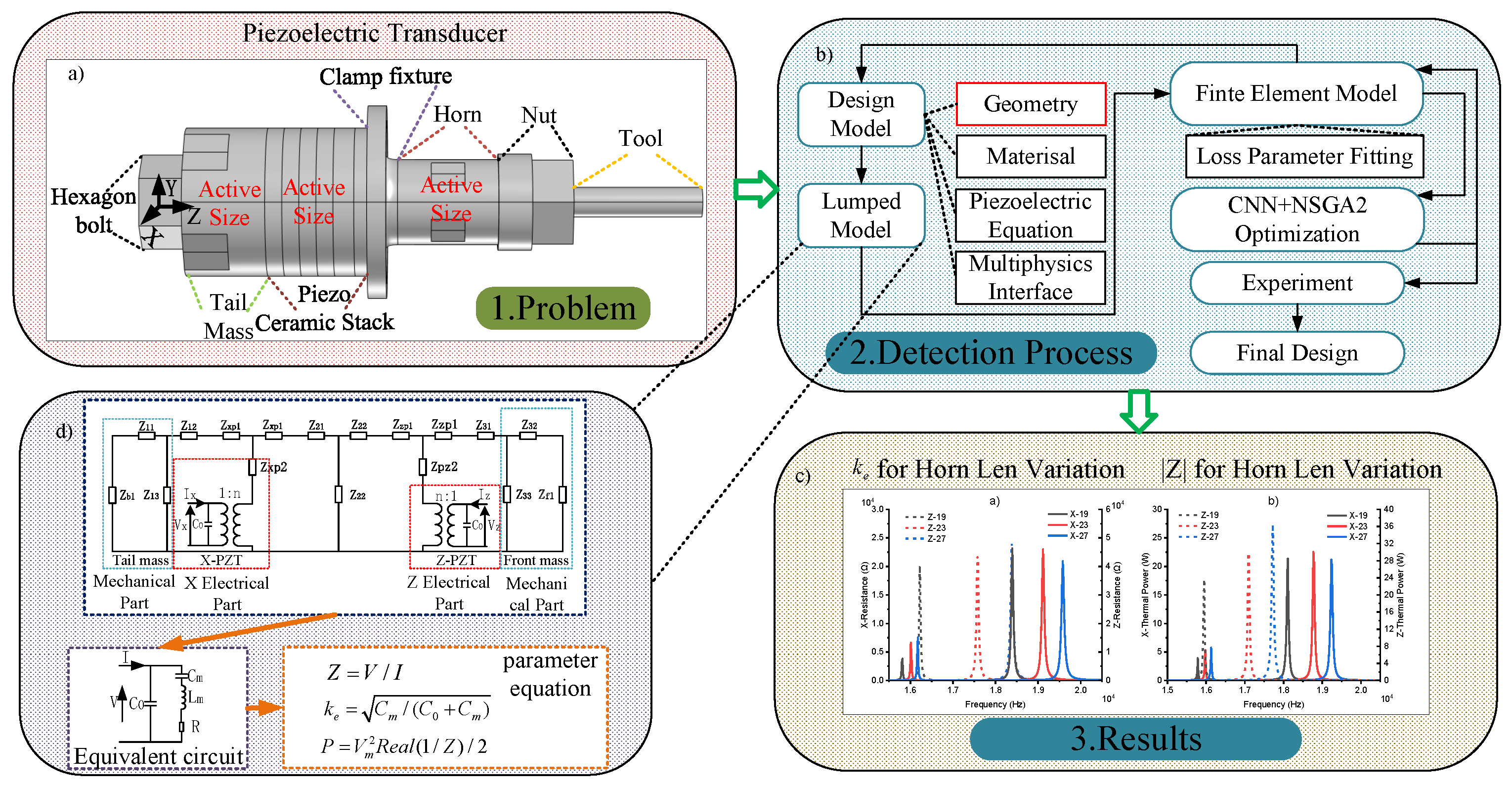
Figure 2.
Lumped model schematic of 3-DOF piezoelectric transducer: (a) schematic of the mechanical structure; (b) lumped-parameter circuit model of the X- and Z-PZT; (c) equivalent circuit of piezoelectric actuator for each axis; (d) polarization directions of the X-, Y-, and Z-PZT; (e) electrical connections.
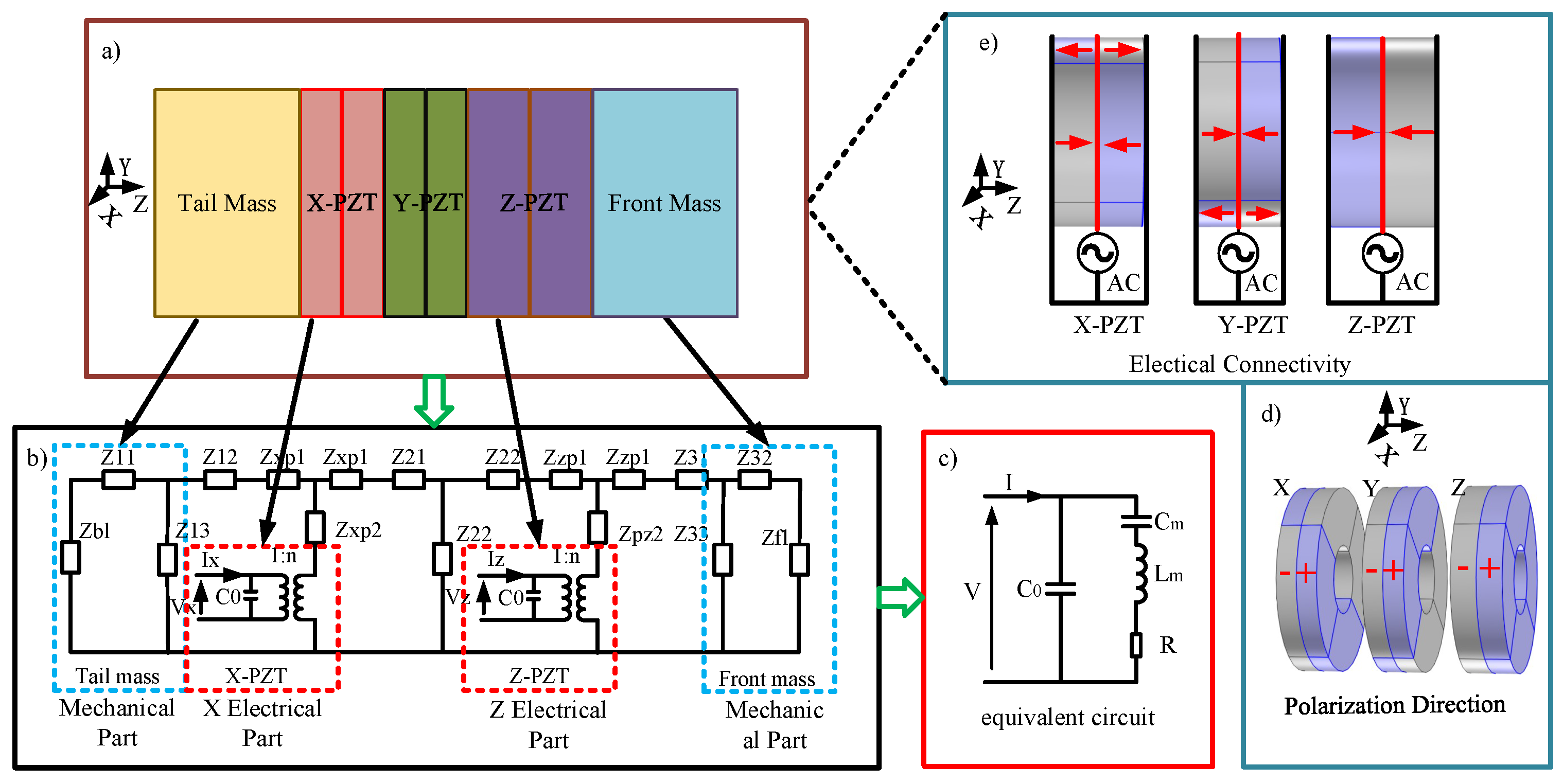
Figure 3.
Detailed schematic of 3-DOF piezoelectric ultrasonic transducer geometry.

Figure 4.
Fitting curve of mechanical loss: (a) X-ufk and Z-ufk; (b) X-|Z| and Z-|Z|.

Figure 5.
Dataset of transducer performance parameters for different geometries: (a) X-ke and Z-ke; (b) X-P.
Figure 5.
Dataset of transducer performance parameters for different geometries: (a) X-ke and Z-ke; (b) X-P.

Figure 6.
Comparison of true and predicted values for the test set: (a) X-ke; (b) Z-ke; (c) X-P.
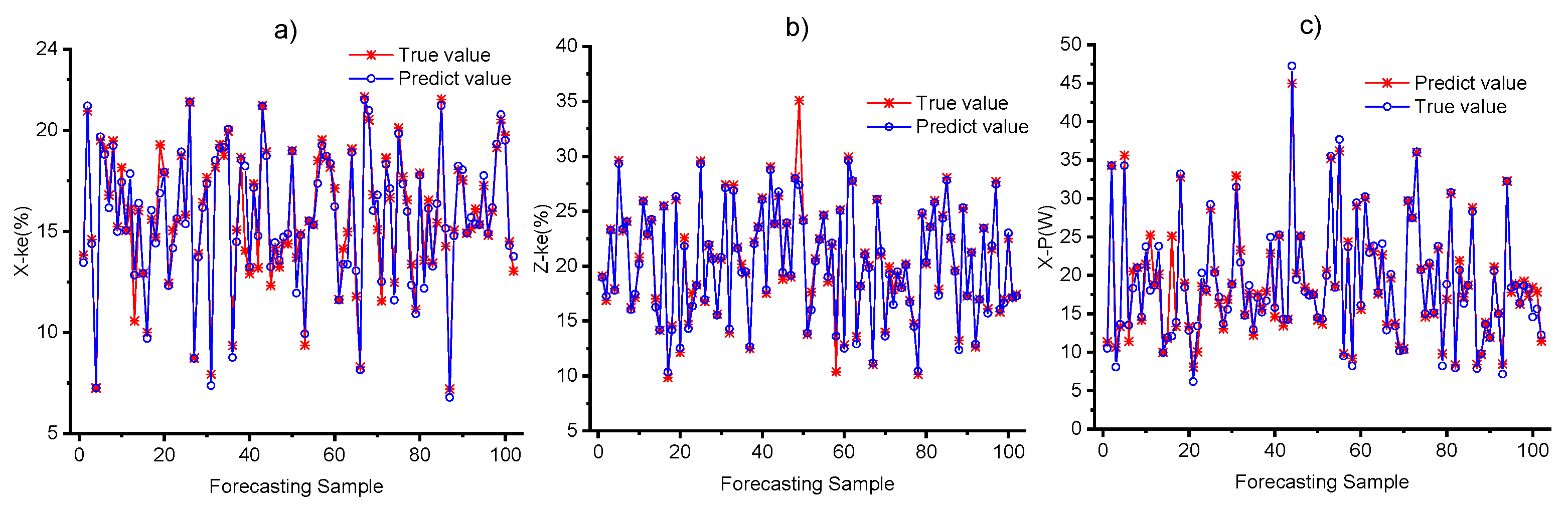
Figure 7.
Flowchart of the NSGA2 optimization algorithm.

Figure 8.
Pareto set of transducer geometrical dimensions obtained by NSGA2 optimization.
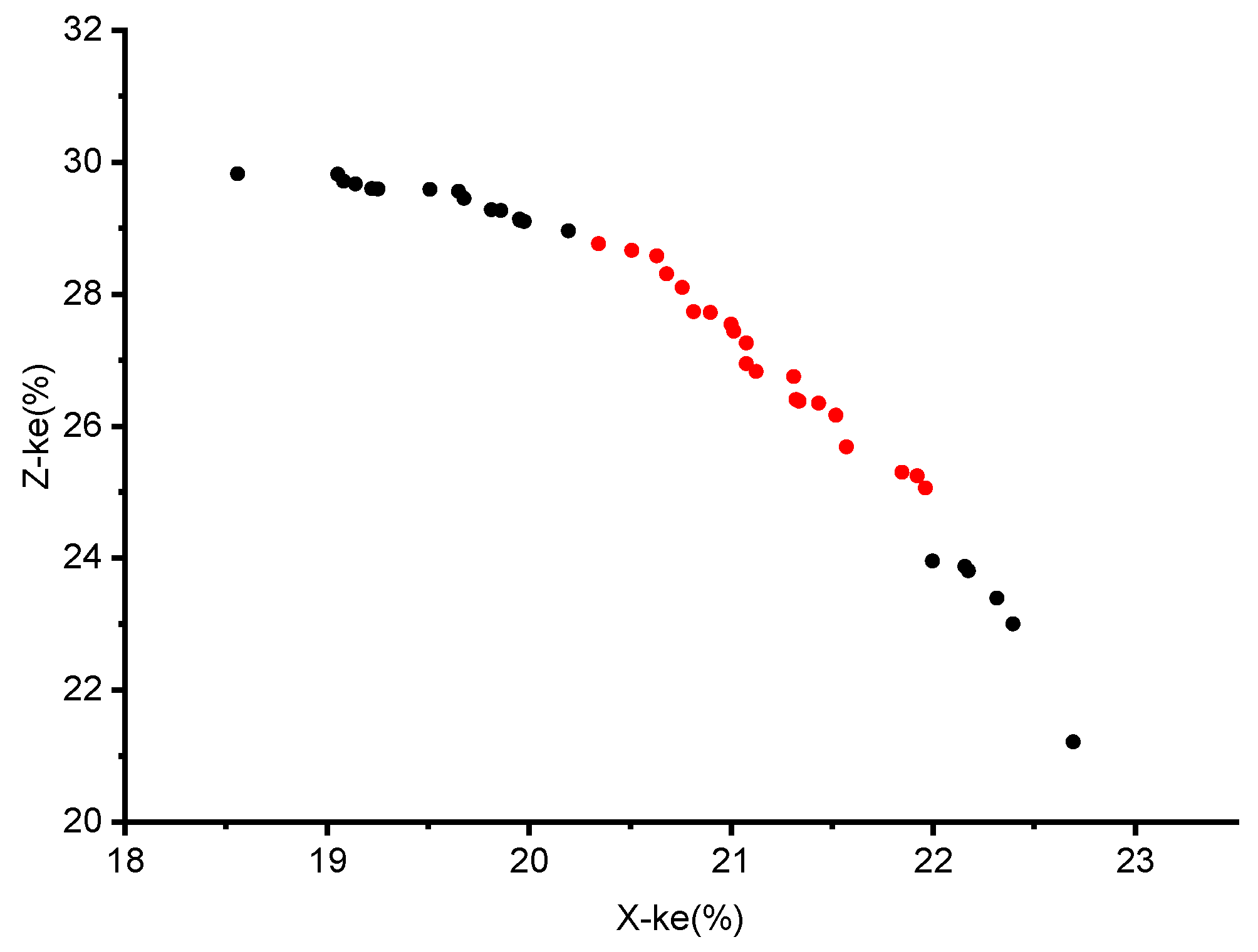
Figure 9.
Length variation of tail mass, (a) X-R and Z-R, (b) X-P and Z-P.

Figure 10.
Diameter variation of the tail mass: (a) X-R and Z-R; (b) X-P and Z-P.

Figure 11.
Length variation of X-PZT: (a) X-R and Z-R; (b) X-P and Z-P.
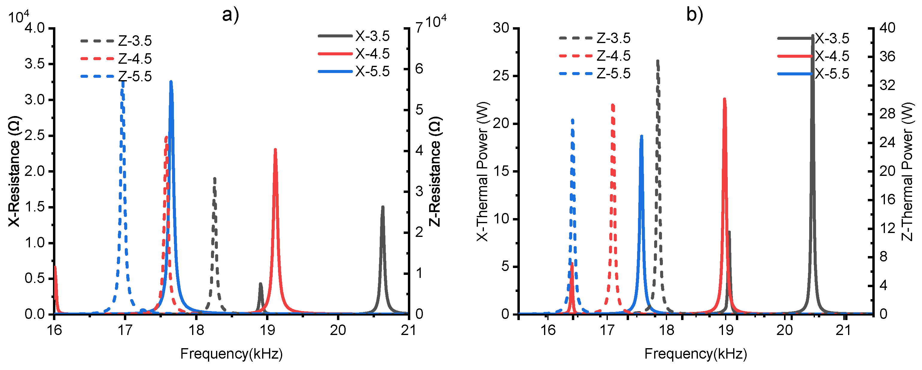
Figure 12.
Length variation of the horn: (a) X-R and Z-R; (b) Z-P and Z-P.
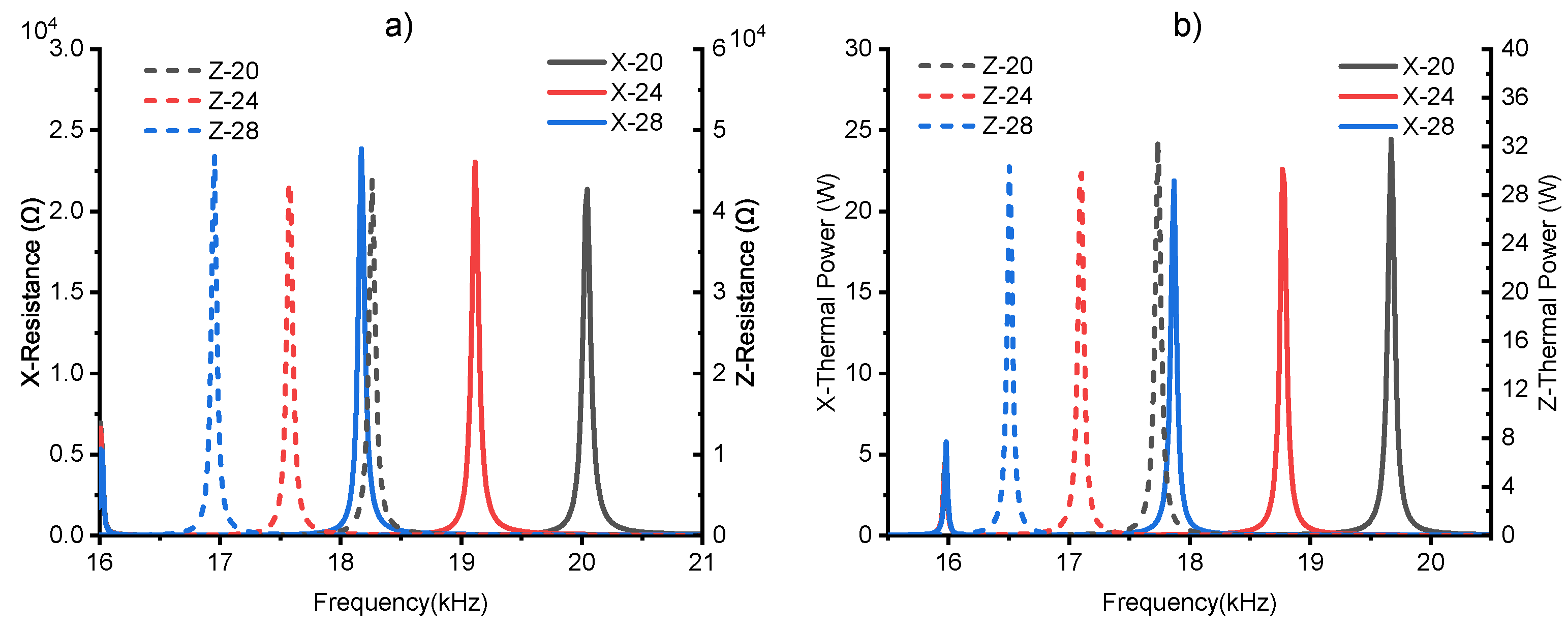
Figure 13.
Diameter variation of the horn: (a) X-R and Z-R; (b) X-P and Z-P.


Table 1.
Geometrical parameters of the 3-DOF piezoelectric transducer.
| Component | Parameter | Unit (mm) | Material | Speed of Sound (m/s) |
|---|---|---|---|---|
| Tail mass | Length | 22 | 304 steel | 5019 |
| Diameter | 40 | |||
| X-PZT | Length | 4.5 | PZT-8 | 3122 |
| Z-PZT | Length | 5.5 | ||
| Horn | Length | 27 | 304 steel | 5019 |
| Diameter | 23 | |||
| Tool | Length | 50 | WC-11 Co carbide | 6709 |
| Diameter | 8 | |||
| Hexagon bolt | Hgrip | 22 | 304 steel | 5019 |
| Hthic | 12 | |||
| Ndia | 15 | |||
| Blen | 57 | |||
| Clamp | Outer diameter | 52 | ||
| Inner diameter | 44 | |||
| Length | 5 |
Table 2.
Physical property of PZT-8 [30].
Table 2.
Physical property of PZT-8 [30].
| Properties | Name | PZT-8 | Unit | Property Group |
|---|---|---|---|---|
| Density | ρ | 7600 | kg/m3 | Basic |
| Flexibility matrix | SE | {1.15, −0.37, 1.15, −0.48, −0.48, 1.35, 0, 0, 0, 3.19, 0, 0, 0, 0, 3.19, 0, 0, 0, 0, 0, 3.04} | (1/Pa) | Strain–charge form |
| Coupling matrix | d | {0, 0, −9.7, 0, 0, −9.7, 0, 0, 22.5, 0, 33, 0, 33, 0, 0, 0, 0, 0} | (C/N) | Strain–charge form |
| Relative permittivity | {1290, 1290, 1000} | Strain–charge form |
Table 3.
Finite element model parameters.
| Geometry Parts | Tmaxerial | Poisson’s Ratio | Density (kg/m3) | Young’s Modulus (GPa) |
|---|---|---|---|---|
| Rear Cover, Clamp, Bolt, Horn | 304 steel | 0.29 | 7860 | 198 |
| Tool [31] | WC-11 Co | 0.25 | 14,440 | 650 |
Table 4.
Seven optimal transducer geometries obtained after managerial decision making.
| Variation | X-- Ture | X-- Predict | Error (%) | Z-- Ture | Z-- Predict | Error (%) | X-P- Ture | X-P- Predict | Error (%) |
|---|---|---|---|---|---|---|---|---|---|
| (22, 40, 5.5, 20, 23) | 22.33 | 21.51 | 3.63 | 25.89 | 26.16 | 1.03 | 18.97 | 19.97 | 5.01 |
| (24, 42, 5.5, 20, 23) | 22.60 | 21.92 | 3.01 | 25.21 | 25.24 | 0.13 | 21.45 | 21.65 | 0.92 |
| (22, 42, 5.5, 25, 27) | 21.29 | 20.81 | 2.23 | 27.64 | 27.73 | 0.33 | 19.19 | 19.50 | 1.59 |
| (22, 42, 5.5, 20, 25) | 21.59 | 21.30 | 1.29 | 26.74 | 26.75 | 0.04 | 20.20 | 20.80 | 2.88 |
| (26, 42, 5.5, 25, 25) | 21.93 | 21.33 | 2.70 | 26.14 | 26.37 | 0.89 | 19.54 | 20.16 | 3.07 |
| (22, 42, 5.5, 20, 23) | 22.50 | 21.84 | 2.91 | 25.09 | 25.29 | 0.83 | 21.75 | 22.07 | 1.45 |
| (22, 42, 5.5, 25, 29) | 20.57 | 20.19 | 1.82 | 28.93 | 28.95 | 0.09 | 18.00 | 18.26 | 1.42 |
Table 5.
Length variation of tail mass.
| Tail Mass Len Variation (mm) | X- (Hz) | X- (Hz) | X- (%) | Z- (Hz) | Z- (Hz) | Z- (%) | X-P (W) |
|---|---|---|---|---|---|---|---|
| (22, 40, 4.5, 24, 23) | 19,115 | 18,770 | 18.91 | 17,585 | 17,105 | 23.20 | 23.20 |
| (26, 40, 4.5, 24, 23) | 18,380 | 18,035 | 19.28 | 17,210 | 16,730 | 23.40 | 23.45 |
| (22, 40, 5.5, 20, 23) | 17,959 | 17,002 | 22.33 | 18,424 | 17,602 | 25.89 | 18.97 |
Table 6.
Diameter variation of the tail mass.
| Tail Mass Dis Variation (mm) | X- (Hz) | X- (Hz) | X- (%) | Z- (Hz) | Z- (Hz) | Z- (%) | X-P (W) |
|---|---|---|---|---|---|---|---|
| (22, 40, 4.5, 24, 23) | 19,115 | 18,770 | 18.91 | 17,585 | 17,105 | 23.20 | 22.59 |
| (22, 42, 4.5, 24, 23) | 19,400 | 19,070 | 18.36 | 17,450 | 17,015 | 22.19 | 20.76 |
| (22, 40, 5.5, 20, 23) | 17,959 | 17,002 | 22.33 | 18,424 | 17,602 | 25.89 | 18.97 |
Table 7.
Length variation of X-PZT.
| X-PZT Len Variation (mm) | X- (Hz) | X- (Hz) | X- (%) | Z- (Hz) | Z- (Hz) | Z- (%) | X-P (W) |
|---|---|---|---|---|---|---|---|
| (22, 40, 4.5, 24, 23) | 19,115 | 18,770 | 18.91 | 17,585 | 17,105 | 23.20 | 22.59 |
| (22, 40, 5.5, 24, 23) | 17,645 | 17,255 | 20.91 | 16,970 | 16,415 | 25.36 | 18.68 |
| (22, 40, 5.5, 20, 23) | 17,959 | 17,002 | 22.33 | 18,424 | 17,602 | 25.89 | 18.97 |
Table 8.
Length variation of the horn.
| Horn Len Variation (mm) | X- (Hz) | X- (Hz) | X- (%) | Z- (Hz) | Z- (Hz) | Z- (%) | X-P (W) |
|---|---|---|---|---|---|---|---|
| (22, 40, 4.5, 24, 23) | 19,115 | 18,770 | 18.91 | 17,585 | 17,105 | 23.20 | 22.59 |
| (22, 40, 4.5, 28, 23) | 18,170 | 17,870 | 18.09 | 16,955 | 16,505 | 22.88 | 21.86 |
| (22, 40, 5.5, 20, 23) | 17,959 | 17,002 | 22.33 | 18,424 | 17,602 | 25.89 | 18.97 |
Table 9.
Diameter variation of the horn.
| Horn Dis Variation (mm) | X- (Hz) | X- (Hz) | X- (%) | Z- (Hz) | Z- (Hz) | Z- (%) | X-P (W) |
|---|---|---|---|---|---|---|---|
| (22, 40, 4.5, 24, 23) | 19,115 | 18,770 | 18.91 | 17,585 | 17,105 | 23.20 | 22.59 |
| (22, 40, 4.5, 24, 27) | 19,580 | 19,235 | 18.68 | 16,220 | 15,950 | 18.17 | 21.20 |
| (22, 40, 5.5, 20, 23) | 17,959 | 17,002 | 22.33 | 18,424 | 17,602 | 25.89 | 18.97 |
Table 10.
Comparing the results of the paper.
| Optimized Structure (mm) | X- (Hz) | X- (Hz) | X- (%) | Z- (Hz) | Z- (Hz) | Z- (%) | X-P (W) |
|---|---|---|---|---|---|---|---|
| (22, 40, 4.5, 27, 23) | 18,169 | 17,804 | 19.94 | 17,038 | 16,539 | 24.02 | 20.38 |
| (22, 40, 5.5, 20, 23) | 17,959 | 17,002 | 22.33 | 18,424 | 17,602 | 25.89 | 18.97 |
Disclaimer/Publisher’s Note: The statements, opinions and data contained in all publications are solely those of the individual author(s) and contributor(s) and not of MDPI and/or the editor(s). MDPI and/or the editor(s) disclaim responsibility for any injury to people or property resulting from any ideas, methods, instructions or products referred to in the content. |
© 2024 by the authors. Licensee MDPI, Basel, Switzerland. This article is an open access article distributed under the terms and conditions of the Creative Commons Attribution (CC BY) license (https://creativecommons.org/licenses/by/4.0/).
Share and Cite
MDPI and ACS Style
Wu, Z.; Zhang, Z.; Wu, D.; Chen, Y.; Hu, F.; Guo, C.; Tang, L. Structural Optimization Study on a Three-Degree-of-Freedom Piezoelectric Ultrasonic Transducer. Actuators 2024, 13, 177. https://doi.org/10.3390/act13050177
AMA Style
Wu Z, Zhang Z, Wu D, Chen Y, Hu F, Guo C, Tang L. Structural Optimization Study on a Three-Degree-of-Freedom Piezoelectric Ultrasonic Transducer. Actuators. 2024; 13(5):177. https://doi.org/10.3390/act13050177
Chicago/Turabian StyleWu, Zhizhong, Zhao Zhang, Deguang Wu, Yuanhang Chen, Fan Hu, Chenxin Guo, and Lijun Tang. 2024. "Structural Optimization Study on a Three-Degree-of-Freedom Piezoelectric Ultrasonic Transducer" Actuators 13, no. 5: 177. https://doi.org/10.3390/act13050177
Note that from the first issue of 2016, this journal uses article numbers instead of page numbers. See further details here.