
Revisiting the Numerical Evaluation and Visualization of the Gravity Fields of Asteroid 4769 Castalia Using Polyhedron and Harmonic Expansions Models

1
School of Astronautics, Beihang Uinversity, Beijing 102206, China
2
Shenzhen Institutes of Advanced Technology, Chinese Academy of Sciences, Shenzhen 518055, China
*
Author to whom correspondence should be addressed.
Appl. Sci. 2024, 14(10), 4058; https://doi.org/10.3390/app14104058
Submission received: 15 March 2024
/
Revised: 18 April 2024
/
Accepted: 30 April 2024
/
Published: 10 May 2024
(This article belongs to the Special Issue Advances in Spacecraft Attitude and Orbital Dynamics, Control, Trajectory Planning and Navigation)
Abstract
:For the convenience of comparison with previous literature, the gravity calculations are revisited for the Asteroid 4769 Castalia, but with extensions on its surface and on intersecting planes and spheres around it, using the polyhedron and harmonic expansion methods with different order and degree for different cases, especially including the gravitational accelerations inside the asteroid, which did not appear at all before. In these evaluations, a few different facts of the these methods and results are revealed, such as the fact that gravity diverges when the position radius is less than the mean radius from harmonic-expansion method, and the maximum gravity is not at the deep valley and mountain top. For a surface that intersects the asteroid, the maximum gravity on it is at the intersection lines between the asteroid surface and the spheres or planes. This means that on the sphere and the plane, the gravities inside and outside the asteroid are smaller than the gravity on the intersection, i.e., on the surface. Some analyses of these conclusions are given with many examples with different radii of the sphere and with different order and degree harmonic expansion models for the above asteroid surface and surrounding spheres. It is interesting to note that very few researchers know that the polyhedral method can also be used to calculate the gravity inside an asteroid with just some modifications of the code. Some special gravity figures on surface and planes inside the asteroid Castalia are computed and made for the first time. The calculations also include tangential gravity, potential, and gravitational slope on surface. Specifically, we find that the overall mean gravitational slope could be one kind of indicator of the density of an asteroid. The minimum overall mean slope happens when the asteroid density is about 2.9 g/cm3, which is much larger than a usually assumed value between 1.7 and 2.5 for asteroid Castalia when its period is 4.07 h, since rotation period should be a more accurate parameter than its estimated density. These conclusions about this typical prolate-like asteroid could be a benchmark for analyzing other similar asteroids.
1. Introduction
Modeling the gravity near an asteroid is important for the study of spacecraft landing, takeoff, hopping and flying around it [1,2,3,4,5,6], etc. Many researchers have studied the gravity fields of the asteroid Castalia for a long time as an example of irregularly shaped bodies. Werner and Scheeres [7] proposed the application of the polyhedral method to evaluate the exterior gravitational field of an irregularly shaped asteroid. The acceleration magnitudes are calculated and compared mainly on different planes, but just outside the asteroid. Takahashi and Scheeres [8] derived the interior spherical harmonic coefficients to model the near-surface gravity of the asteroid. And recently, J. Sebera and A. Bezdek [9] calculated the gravity field of Castalia using spheroidal modes to increase precision. But no literature shows the figures of gravity on the surface and on the planes and spheres inside the asteroid Castalia.
Other researchers utilize the triaxial model [10,11] and the masscon method [12,13] to calculate the gravity of an asteroid. Recently, the gravity of asteroids has also caught the attention of researchers outside of aerospace engineering, such as those in astronomy, astrophysics [14,15], geology, geophysics [16,17], and others. These researchers are particularly interested in the internal gravity of asteroids and have begun using CFD with a variable density approach. However, the most commonly used methods are still the polyhedral and spherical harmonic expansion due to its precision and speed, respectively.
In this paper, the gravities on the surface of the asteroid and on spheres around the asteroid, as well as cross-sectional planes, including the internal gravity, are calculated using the classical polyhedral method and the harmonic-expansion method. For the convenience of comparison to previous literatures, the asteroid Castalia is used again as an example. Many interesting conclusions are given. Some special physical perspectives are revealed.
The remainder of this article is organized as follows. Section 2 introduces the method harmonic expansion and polyhedral method briefly with some comments about their special applications in this paper. In Section 3, after we introduce some fundamental parameters of the typical prolate-like asteroid Castalia, the 3D and 2D shapes of the asteroid are plotted first, and then the harmonic expansion coefficients of the asteroid and a rectangle up to the sixth degree and order are calculated. In Section 4, many examples of gravitational accelerations, both on the surface of and spheres around the asteroid and on planes intersecting the asteroid, are calculated. Here, we assume that the asteroid has constant density. Comparisons are also performed. Finally, Section 5 gives the conclusions and explanations.
2. Gravity Calculation Method
The spherical harmonic gravity field is widely used with coefficients associated with Legendre functions of degree n and order m [18] and its application to asteroid [2,19].
where r is the radial distance from a given point to the centroid of the asteroid. is its latitude, and is the longitude. G is the gravitational constant, M is the total mass of the asteroid, is the reference radius, is the normalized associated Legendre function of degree n and order m, and and are the normalized spherical harmonic coefficients:
where are radius, latitude, longitude, respectively of a distributed mass inside an asteroid. And if ; if . The is the same reference radius in Equation (1). By comparison, the reference radius can apparently be chosen arbitrarily, but it is normally chosen as the mean radius of the asteroid, i.e., the radius of a corresponding sphere with the same mass as the asteroid. The mean radius is an important parameter of the asteroid. Similar to the Earth, at positons where , it can be regard as the “sea level”; for , it is the “land area”; and for, , it is the “ocean floor”. This classification is helpful to discuss the convergence and divergence regions of the harmonic expansion examples of an asteroid’s gravity, which will be discussed comphrehensively in the following sections.
2.1. Polyhedral Method
For the polyhedral gravity field, the potential of spacecraft at position r is [7]
where the density is assumed to be a constant and r is a vector from the field point to any point on edge e. r a vector from the field point to some fixed point in the face plane f. Suffixes e and f denote the edge and face of the polyhedron. The face’s outward-pointing normal vector is , and its dyad and is outward edge normal, which is on the plane f and perpendicular to the edge e. For the edge connecting vertices i and j shared by faces A and B, the edge dyad is , with similar s. If is the vector form of the spacecraft-to-polyhedron vertex , is its magnitude. is the length between vertices and , and an edge factor is defined as
is a dimensionless face factor bounded by the triangular face f:
We note that many researchers know that the polyhedral method can calculate the gravity outside or near the surface of an asteroid. Some of them may know that it can be used to calculate the gravity even on the surface. But very few of them know that it can calculate the gravity inside the asteroid with some modification of the codes.
2.2. Gravitational Acceleration and Coordinate Transformation
As the spacecraft’s gravitational acceleration is normally no longer on the radius directions for irregular asteroid, in the calculations in this paper, some transformations are needed from spherical coordinates to Cartesian coordinates. The gravitational acceleration and related symbols = are
where ,, . But the magnitude square of the gravitational acceleration a can be simplified as
3. Asteroid Castalia Shape and Some Parameters
Some parameters are listed here for Castalia that are similar to the data in reference [1]. Density is assumed to be 2.1 g/cm3, and total mass km. Castalia is a typical prolate asteroid, which probably evolved from a contact binary. The maximum and minimum radius r and are, respectively, , , , . Figure 1 and Figure 2 show the computer model and its radius contour of Castalia’s shape. Compared with the figures of Castalia in previous studies, more details can be found in this three-dimensional (3D) shape and two-dimensional (2D) contour maps. The small red dot line in Figure 1 denotes the reference radius , which will be used later. The red dashed line in Figure 2 also represents the reference radius km. The thick red lines in the two figures denote the intersections of teh three planes, , with the asteroid’s surface, which divide the asteroid into eight parts.
The normalized spherical harmonic coefficients (6 × 6) are listed in Table 1. But and from 0 to the order 16 are obtained by calculating a shape model with 2048 vertices, 4092 faces, and 6138 edges [20]. Higher-order terms will be used later in this paper. The first (4 × 4) results are quite similar to the coefficients in paper [1]. The largest two terms are , except the constant . The other terms are just half of the two or less in magnitude. On the whole, is much larger than Interested readers can find that the magnitudes of , , are not very small and are even larger than the magnitude of , which has the biggest value in terms of degrees, respectively. By careful examination of the shape of Castalia and the spherical harmonic coefficients in Table 1, we find some shape characteristics of triangle, square, and pentagon, which have more harmonic coefficients than a hexagon. This is one reason that we show the coefficient to 6th order here.
When we discuss the surface gravity of Castalia, the maximum value appears at the center of some surface part that is nearly a plane. This is similary to a rectangle. Actually, the gravity about a rectangle was studied long time ago using the analytical method [21]. Hence, we also calculate both the gravity and the spherical harmonic expansion coefficients for a simulated rectangle, which are list in Table 1. In the table, we can see that second-order coefficients are almost the same, and the fourth-order coefficient is also similar to some degree. But for the sixth order, even the positive and negative signs are different. A comprehensive analysis of the gravity of a rectangle will appear in an upcoming theoretical paper on gravity.
4. Calculation Results and Analysis
Some parameters are computed in this section, which include gravity potential, total gravitational acceleration, tangential acceleration, and surface slope with respect to local gravity level.
Practically speaking, the potential on the surface is the minimum energy for landing on the asteroid from infinity or leaving the asteroid to infinity. Internal gravitational acceleration determines the stress and strain of the structure of asteroid. Outside acceleration determines the orbits of a probe.
Slope is important for the analysis of dust motion on the surface of an asteroid because the tangent of this angle is equal to the steady friction coefficient of dust on its surface. As a byproduct, the calculation of the overall mean minimum slope can be an constraint of the free density parameter. The surface gravity magnitude is used to calculate the landing and take off of a probe on the asteroid.
When we calculate the orbit around an asteroid, the landing and taking off, or the hopping on surface, we often meet the following kind of problems: (1) When do we have to use the time-consuming polyhedral method? (2) When can we use the fast spherical harmonic model? (3) How do we simply choose a good enough order and degree of spherical harmonic model? Rather than consider the abstract definition of the exterior Brillouin sphere, though it is sometimes regarded as the circumscribing sphere, km for Castalia [8,9], in this paper, we use the direct parameter, mean reference radius , to find some criteria to answer above practical questions.
We also apply the conventional polyhedral model [7] without much modification of the algorithm to calculate the gravitational acceleration inside an asteroid without considering the internal Brillouin shpere. This could be a surprise for most researchers. We also use this polyhedral model to compute the gravitational acceleration on the surface of asteroid without using the special type interior/exterior spherical Bessel gravity fields [8]. In this circumstance, the polyhedral method also works well, which is known by very few researchers.
In this section, through many detailed computations regarding asteroid Castalia, we quantify the performance of the polyhedral method for internal and surface gravity. By comparison of its results to harmonic expansion with a different order and degree, recommendations are summarized in order to help planning of proximity operation for future missions to this kind of typical prolate asteroid. Many illustrative computation figures are shown, many of which did not appear in previous studies.
4.1. On the Asteroid Surface
There are a few reasons to make many kinds of calculations about the asteroid surface. First, it is required for practical applications, such as landing and taking off. Second, it can give readers a direct physical sense of some parameters. Third, it is easy for comparisons, such as the choice of order of harmonic expansions, since we assume the polyhedral results as the standards for comparisons.
4.1.1. Gravity Potential and Acceleration by Polyhedral Model
Figure 3 shows the gravity potential on surface of the asteroid. The unit here is 102 cm2/s2 = 10−2 m2/s2 = 10−8 km2/s2. And the intersections between the principal plane , equatorial plane , and zero longitude plane with the surface are also shown in red dash lines in Figure 4. Here, the density is 2.1 g/cm3. The calculation results are important for the analysis of a probe’s taking off or landing and especially for the estimation of the energy needed from the surface to infinity. Interested readers can compare this figure with the gravitational accelerations in Figure 5. The larger the potential, the smaller its gravitational acceleration, as we expected, since the value is more closely related to its shape; see Figure 1 and Figure 2. Because the potential is inversely proportional to its radius, the zero potential is defined at infinity as usual.
Figure 4 shows the contour of the potential on the surface, longitude vs. latitude(deg), which corresponds to the magenta lines in Figure 3. The thick red dashed lines are the intersections of the plane with the surface of the asteroid. The minimum values are the longitude and latitude, (−100, −20), (−40, −75), (−120, 70) deg, which are the nearest points to the center of mass. The maximum values are roughly at (170, 8) deg at the farthest point from the center of mass. These are physically correct. On the whole, the farther from the center, the larger the potential, and the nearer to the center, the smaller the potential. But for acceleration magnitude, it is not in the exactly the same inverse case: the farther to the center of mass, the less its acceleration, the nearer to the center, the larger its acceleration. The largest potential corresponds the minimum gravitational acceleration, but the smallest potential does not correspond to the largest acceleration. See Figure 5 and Figure 6.
Figure 5 shows the 3D gravitational acceleration for Castalia on the surface based on the polyhedron method. The acceleration unit is 10−5 m/s2. The thick red lines are the trajectory, where the radius of the asteroid is equal to the reference radius km, i.e., the intersection of the sphere with radius with the asteroid’s surface. The mean value of acceleration is 29.0, the maximum is 30.5, the minimum is 25.5, and the variation is 1.1. Hence, the gravitational acceleration on surface changes slightly on the whole.
Figure 6 presents the contour of the gravitational acceleration on the surface of Castalia based on the polyhedron method. The thick red lines are also the trajectory on the surface where the radius of the asteroid is equal to the reference radius, km. The unit here is 10−3 mgal (1 mgal = 1 cm/s2 = 10−5 km/s2). To give a rough overall description of the gravitational acceleration, we assume that its shape is a rectangle. The largest values appear near the centers of the plane, and its longitude and latitude are about (60, −30), (−50, −20), (−20, 70), (180, −80), etc. The smallest values appear near the corners, such as (−80, 10), (40, 20), (10, 15), (160, 10), (−140, 15), etc. This is one reason we calculated the harmonic expansion coefficients of a rectangle in Section 3 to deeply understand the relation.
4.1.2. Harmonic-Expansion Method
With the polyhedral results of the gravitational acceleration on the surface of the asteroid, we can evaluate the harmonic expansion computation with different order and degrees. We give the calculation with the order and degree of 4 × 4, 6 × 6, 10 × 10. This give us a direct physical sense to choose the order and degree of harmonic expansion. Nevertheless, the polyhedral method’s computation cost is too much higher than that of the harmonic-expansion method. If the probe’s radius is a little bit larger than the reference radius, a 10 × 10 order and degree harmonic expansion is good enough, and for a rough analysis, 4 × 4 is enough. If the probe is far enough, say, from the center of mass, all methods will obtain similar results. This means the 4 × 4 harmonic expansion is best because it is fast and simple. For all the comparisons here, the homogeneous-density polyhedral gravity field is treated as the truth model since it works anywhere outside, inside, and on surface of an asteroid.
Figure 7 shows the gravity field of the sixth degree and order for Castalia on the surface. For the “land areas” where its radii are larger than the reference radius , the calculated gravitational accelerations are acceptable (within 5% error), whereas on the “ocean floor,” where their radius is less then that of reference , which can be compared with the “sea level” of the Earth, the gravity calculated by harmonic expansion is much amplified by up to 6 to 8 times larger than the corresponding value from the polyhedral method, which is assumed as a true value. Hence, in this case, the results are completely meaningless. Apparently, we can choose a different reference radius to change the convergence problem. Actually, this radius is better determined by the inherent mean radius, which correspondsto a sphere’s radius, which has the same mass as Castalia. Hence, it is not an arbitrarily chosen value. This is a fundamental invariant limitation for the spherical harmonic-expansion method, no matter which number is chosen as the reference radius because any number can be transformed to this value with a ratio and cancelled by corresponding harmonic coefficients. This means the larger the chosen, the smaller the values of and .
Interested readers can find a detailed comparison in the contour map Figure 2; i.e., in deep valleys of the ocean, the contours are quite similar, which means that the gravitational accelerations are mainly determined by the radius at these places, where the radius is much smaller than the reference radius. It can be seen that the maximum acceleration at the high-latitude region, where the radius is at a minimum, approximates to the value near the crevice between the two Castalia’s lobes. This is all because the harmonic-expansion method diverges in these regions. The exterior gravity field is roughly valid outside the reference radius . For the part inside the reference radius, the acceleration errors are larger than what is acceptable. The average mean acceleration on the surface of the asteroid is about 30 × 10−5 m/s2. At the north and south pole and near the crevice, the calculated value is high at up to 200.
Figure 8 shows the gravitational acceleration of the fouurth degree and order for Castalia on surface, and Figure 9 shows the gravitational acceleration of the 10th degree and order for Castalia on the surface. This is very close to the polyhedron results in Figure 6 at the corresponding surface where , i.e., inside the thick red boundaries, with only about 1–3% difference. And the higher-order model can help to increase the accuracy on the surface when its radius is larger than km. It is important to note that the large errors are contained only in regions where on the surface. And the high-degree model yields larger acceleration errors than a low-degree gravity field when since the term s in Equation (1) causes the divergence. A larger n brings larger error. Simply speaking, a higher-order spherical harmonic expansion model can make convergence region more accurate, at the same time making the divergence region even deteriorate more than the lower-order model.
4.1.3. Gravity Tangential Acceleration and Slopes
Figure 10 shows the surface tangential acceleration when the asteroid does not rotate. We see the largest accelerations appear at the crevice between the two lobes, around a bottom crater (−40, −80°), and around a top crater (150, 70°) in a circle form in the longitude vs. latitude space.
Figure 11 shows the contour map of the surface tangential gravitational acceleration when the asteroid does not rotate. It is noted that the overall pattern of figure is quite similar to the gravitational slope: as the surface gravity does not change much, then the tangential gravity is roughly proportional to the slope since the slope is not large. If the tangential gravity is zero or small, i.e., in the dark blue region, then the attraction and normal force vectors are anti-parallel. Dust near these places can exist, because when the tangential gravity is small, the motion of a loose particle is controlled by the coefficient of friction between the particle on the asteroid surface. If there is a place whose tangential gravity is large, there is no loose particle here, it is probably a rocky place without dust. Note that the two lobes are widely separated at yellow crevice region, a longitude of −100°, and a latitude from −40 to 40°; hence, an influx of a regolith may not be adequate to fill in this crevice, even over long time spans. Hence, in the yellow regions, a dust cannot exist; it must be stony in these areas. These calculations can help us to discriminate which parts of the asteroid is dusty or stony.
Figure 12 shows the surface tangential gravitational acceleration when the asteroid rotates at a period of 4.07 h. This time, the acceleration acting on a dust at each location on the surface of the asteroid arises from both the gravitational and the centripetal accelerations. We see that the overall gravity is obviously smaller than the gravity without rotation. Dust motion is reduced. Dust only appears at the place where the tangential gravity is small. This can help us to choose a landing site where tangential gravity should be small, since the place is rocky where its tangential gravity is large. When an asteroid rotates slowly, the gravitational attraction between the particles can hold them together. But if it rotates fast enough, the centrifugal forces would even overwhelm the gravitational pull and rip the rocks apart. Figure 13 shows the contour of the surface’s tangential gravitational acceleration when the asteroid rotates at h. The largest value here is 14 mgal, whereas its value is 18 for case with no rotation, though the overall pattern is similar. See Figure 11.
Figure 14 shows the surface’s effective slope when the period is 4.07 h for asteroid Castalia. Here, the density is 2.1 g/cm3. It is the angle between effective gravity and the negative local surface normal, i.e., the angle between the local surface horizon and the local gravity horizon. This angle is a practical definition to analyze the dust motion on surface. If the value is small, the dust can be motionless because of friction. If the value is large, say 33°, ([22]), the friction cannot resist the tangential force to move the dust.
Figure 15 shows the 2D contour of the slope, which is completely different from results in FIG.14(P.80) in reference [1]. This is also a reason we revisit the gravity of Castalia in this paper. At the crevice where the longitude is about −90 deg between the two lobes of Castalia, the slope is large. The overall pattern is quite similar to the tangential acceleration. See Figure 13, as the total surface gravitational acceleration does not change much. To easily describe the overall pattern of the slope, we assume the shape is a rectangle. On the top and bottom surfaces, i.e., where the latitude is greater than 25 deg and less than −30 deg, the whole slope is about 10 deg, except fortwo craters, one at (170, 80) and one at (−40, −80). On the side, in the middle area, i.e., the equatorial strip, the slope is very small, less than 5deg. In the regions up near the edge, i.e., where the latitude is about 20 deg and and −25, the slope is large, about 25 deg. This slope distribution is quite different from the slope of the asteroid Bennu [23], which is a nearly circular oblate asteroid.
Figure 16 shows the histogram of the acceleration slope. In the shape model, there are a total of 2048 vertices and 4092 faces for the asteroid Castalia. The vertical axis is the number of the faces, and the horizontal axis is the surface slope with respect to local gravity horizon direction for each face. In the figure, the number of faces vs. the gravitational slope for rotation (brown) and no rotation (blue) case are presented. We see that the number of faces shifts to left because of the rotation, which means the overall gravitational slope is smaller for the rotation case.
The overall mean slope is 12.89 deg for the rotation case when its period is 4.07 h. The overall mean slope is 15.28 deg for the case with no rotation. More calculations show the mean slope for a different rotation period. The results are as follows: slope(period), 81.26 (2 h), 29.50 (3 h), 12.89 (4 h), 11.48 (5 h), 12.25 (6 h), 12.98 (7 h), 15.28 (infinity), and (rho = 2.1).
Here, we choose a density of 2.1 g/cm3; actually, the density could be between 1.7 and 2.5. From our analysis, the density should be larger than 2.1. A more reasonable value is 2.9, because the minimum mean slope appears when the period is 5 h in this calculation. More tests show that when the density is 2.9, the overall mean slope is at its minimum when the period is still 4.07 h, i.e., the mean effective slope (density) 12.57 (2.1), 11.75 (2.4), 11.46 (2.7), 11.43 (2.8), 11.32 (2.9), 11.43 (3.0), 11.53 (3.3).
Since the period is estimated relatively more accurately using a light curve, the density could be higher than the usually assumed value of 2.1 g/cm3. Hence, the overall mean slope could be used to estimate the density inversely. This could be an important conclusion of this paper. Since the asteroid Castalia’s shape is bifurcated into two distinct lobes (stones) separated by a crevice, its porosities could be more stony irons of 60 percent than the ordinary chondrites of 40 percent. Previous studies have assumed a maximum slope of 33 deg before slipping occurs (Thomas et al., 1994) [22]. All the slope values computed here are less than 33 deg when the the case period is 4.07 h and the density is 2.1 g/cm3, except when there are five faces. The 5/4092 faces greater than 33 deg are 33.4364, 33.7655, 38.9643, 34.0522, 35.0978 deg, where they could be smooth rocky surface areas without dust on them or where cohesive forces exist to help hold them together.
Note again that the estimation of the density from the gravitational slope is a suggestion or a guess. Since density is one of the most difficult parameters of an asteroid to estimate before a spacecraft flies near it, any suggested approach to estimate density is valuable. We find that the overall gravitational slope could be a indicator of the density at some degree. This is an important contribution of this paper. Here, we can give more explanation of this point. If the asteroid is a sphere, then the gravitational slope at any point on the surface of the asteroid is zero. Free dust always tries to stay at a place where the gravity is small. Hence, different density can lead to differences in the overall mean gravitational slope. There is a minimum point of overall gravitational slope with the variation of density.
4.2. Gravity on Spheres Intersecting or Outside the Asteroid
There are a few reasons to calculate the gravity on a sphere. First, since all the radius distances are the same, one degree of freedom is removed, and many kinds of comparisons become easy. Second, many real spacecraft missions such as satellite gravity survey, navigation, and remote sensing tasks are designed on circular or near circular orbits. The third reason is that it can be used as a kind of visualization strategy for the gravity experienced by a spacecraft. We calculate the gravitational magnitude for different radius, , , , by the 4th, 8th, 16th order and degree harmonics models and the polyhedral model in this section. Based on all these calculations, we can answer the frequently asked questions by application engineers about which model is the best choice when we calculate the gravity of a typical asteroid under different conditions.
Figure 17 shows the gravitational acceleration obtained by the polyhedron model for Castalia at the sphere of the r = 0.5431 km radius. The gravitational acceleration unit here is mgal, where 1 mgal = 10 m/s2 = 10 km/s2. Special attention should be given to the fact that the blue boundary on the red edge is on the surface of the asteroid. Inside the boundary, the gravity is inside the asteroid, which is smaller than the corresponding place with the same radius on the surface. This is physically correct. So we can visualize the gravity inside the asteroid, which is helpful to understanding the evolution of the asteroid. This sphere includes both the inside and outside parts of the asteroid.
Figure 18 shows the gravitational acceleration by the potential of the fourth degree and order for Castalia on the sphere r. The unit here is mgal. The axes are the longitude and latitude, respectively. The sphere with radius r intersects the asteroid. Some part of the sphere is outside the asteroid, and the other part is inside the asteroid. We see the gravitational acceleration at the points where the surface radius of the asteroid is larger than cannot be acceptable. Actually, the sphere at these part is inside the asteroid. Comparison can be made to Figure 17.
Figure 19 and Figure 20 show the gravitational acceleration of polyhedron model and by the potential of the fourth degree and order for Castalia at the distance of 2 r, which is just outside the Brillouin sphere. The unit is 10 m/s2, on average, approximating 8 m/s2 acceleration. The unit here is mgal (1 mgal = 10 km/s2 = 1 milligals = 10 m/s2 = 10 cm/s2). The axes are longitude and latitude, respectively.
Figure 21 and Figure 22 show the gravitational acceleration by the polyhedron model and by the potential of fourth degree and order for Castalia at a distance of . The unit is 10 m/s2. On average, the overall mean value approximates 3.6 m/s2. The axes are longitude and latitude, respectively. The difference between these figures becomes smaller compared to the case when based on these two methods.
Figure 23 and Figure 24 show the gravitational acceleration of the polyhedron model and by the potential of the fourth degree and order for Castalia at a distance of 4 r. The unit is 10 m/s2. On average, the value approximates 2.0 m/s2 in acceleration. The axes are longitude and latitude, respectively. At this radius, radial gravitational acceleration dominates in the whole magnitude of acceleration.
Figure 25 shows the gravitational acceleration in the eighth degree and order model for Castalia on the sphere 2 r, which is just outside the Brillouin sphere. The unit here is mgal (1 mgal = 10 km/s2). A comparison can be made with Figure 19 and Figure 20. We can see that the 8 by 8 model is more accurate than the 4 by 4 model. Figure 26 also shows the gravitational acceleration in 16 degrees and the order model of spherical harmonic expansion on the sphere of 2 r. The unit here again is also 10 m/s2. There is very little improvement in the accuracy of the 16 × 16 model compared to the 8 × 8 model.
By all these comprehensive calculations, we can conclude that only the polyhedral model works inside reference , and the harmonic expansion is accurate enough when the position is far enough, say 4 , and when the position is near the surface but outside the reference radius , the higher-order model is better, say , or at least or .
4.3. Gravitational Accelerations on Intersecting Planes
These results inside the asteroid show the power of the polyhedral method for a typical highly non-spherical asteroid.
Figure 27 shows the magnitude of gravitational acceleration on the plane , i.e., the equatorial cross-section when the asteroid Castalia does not rotate. The largest gravity appears at the surface, as the white dot line indicates. The density is chosen to be a constant, 2.1 g/cm, in all the gravity calculations, as is usually assumed.
Figure 28 also shows the effective gravity on the plane , when the asteroid rotates. Castalia rotates about its Z axis with the maximum moment of inertia. This time, the force acts as a motionless dust, , which could be inside, outside, or on the surface of the asteroid, which arises from both the gravitational and centripetal accelerations. , , and are calculated using the polyhedral method. We can see five equilibrium points, one stable inside and four unstable outside. The rotation period of Castalia is still 4.07 h. The outside equilibrium points are compatible with the analysis in paper [3] with just two gravity harmonic parameters and , which are all unstable. In the paper [3], we found four equilibria: the two on the x-axis are always unstable, and the two on the y-axis are sometimes stable and sometimes unstable. We also derived stability conditions. But we do not disscuss the stability of the equilibrium inside the asteroid. These conclusions agree well with the calculations in this paper with a polyhedral model. We can see the direction of the gravitational acceleration arrow from Figure 29, showing that all four equilibria are unstable, and the one inside is stable. This can ensure that the dust on surface does not fly away. These numerical calculations validate the zero-velocity analysis in reference [1]. Also, the overall gravity near the surface is smaller than the gravity without rotation; see Figure 27, because the maximum gravity, which should appear on the surface, becomes smaller.
More specifically, Figure 29 shows the direction distribution of the effective acceleration in the equatorial cross section plane, , when the asteroid rotates. This is also dust moving in the direction without initial velocity in the rotating asteroid, corresponding to Figure 28. Inside the dark blue ring, where the acceleration value is 4.8, dust will move downward, whereas outside the dark blue ring, dust will move outward. The ring could be regarded as an outside protection boundary layer of dust on the surface of the asteroid. Inside the asteroid, we can see the deformation vectors on the cross-section where the white dashed line is the surface boundary.
Figure 30 shows the gravitational acceleration on the plane when the asteroid does not rotate. The dotted white lines represent the intersection between the asteroid’s surface and the principle plane . On the plane , the acceleration is nothing special, so it is not shown here.
Figure 31 shows the gravitational acceleration, also on the plane , but when the asteroid rotates, with three equilibrium points, one inside and two outside. The white dot outline represents the intersections of Castalia’s surface with its principal planes, plane , i.e., the plane.
5. Conclusions and Discussion
We have evaluated the gravitational field environment around a typical two-lobe configuration prolate asteroid, Castalia, on its surface and also outside or inside its surface, with different planes and spheres.
The gravitational field expansions on the surface and on spheres intersecting or outside are compared against the polyhedral gravity field model constructed from a homogeneously distributed body. Also, the gravitational accelerations in cross-sectional planes show the internal gravity, which can only be calculated using the polyhedral method. This paper studied the gravity characteristics of Castalia in depth using various kinds of examples.
The accuracy of the harmonic-expansion gravity field deteriorates for the disfigured asteroid Castalia inside the mean reference radius, and the potential and acceleration errors for a 4 × 4, 6 × 6, and 10 × 10 expansion exceed well over 2 or even 10 times their assumed true value from the polyhedral model. As the harmonic-expansion gravity field suffers from the convergence problem within the mean reference sphere, the exterior gravity field should not be used to model the gravitation near or on the surface of the body where .
The surface gravitational acceleration on an asteroid can be divided into two convergence and divergence regions if calculated by harmonic expansions. Regions whose radius r are larger than the mean radius of the asteroid are the convergence regions and vice versa. This radius is not the arbitrarily chosen reference radius for the harmonic expansions, but it is sometimes chosen as the mean radius.
The polyhedral method can be used to calculate the gravitational acceleration outside, inside, and on the surface of an asteroid, but the calculation run time is much longer than the harmonic-expansion method. For a common personal computer, the CPU calculation time for the surface gravitational acceleration is a few minutes for the harmonic-expansion method but a few hours for polyhedral model with 4092 faces. Recently, some approximate and hybrid models were utilized to reduce the CPU runtime [24] at the cost of losing some accuracy, especially near the surface of the asteroid. Off course, there are some other researchers also address this issue [25,26].
A few special qualitative comments can be summarized as follows.
- (1)
- If the calculated sphere’s radius is larger than the maximum radius of the asteroid, for example, if the radius is greater than 2 = 1.0862 km here, the gravity harmonics work as well as polyhedron method; the farther the better, and the higher the degree the better. The sphere with the maximum radius of the asteroid is the so-called Brillouin sphere [8]. The maximum radius for the asteroid Castalia is 0.851 km. See Equation (1), for all the calculated spheres with the radius , , for both the polyhedral and spherical harmonic models.
- (2)
- For preliminary analysis, the 4th-order and degree gravity model is good enough, especially for spheres with , and not much of an obvious difference can be obtained by using the 8th- or 16th-order model or the polyhedron method with less than 1% error. The farther from the asteroid, the lower the order of the coefficient dominating the gravity. See Figure 20, Figure 25 and Figure 26, etc.
- (3)
- On surface points where the radius is less than the reference radius and the points inside the asteroid, only polyhedron method can obtain reasonable results.
- (4)
- For the points outside the asteroid or on the surface of the asteroid, if its radius is greater than reference or less than its maximum radius, the harmonic expansion model still works with relatively large errors but still with acceptable accuracy; i.e., it still converges with 5% error, and the higher order of the model of harmonic functions, the closer to the polyhedra model’s results. See Equation (1), . As all the coefficients and are much less than 1, and for the normalized Legendre polynomial , it is easy to understand that all the points with converge.A rough proof for understanding the above comments is as follows.
- (5)
- Again, more clearly, if the radius is inside the Brillouin sphere, say km for Castalia, but larger than its mean reference radius, km, the spherical harmonic-expansion method still works, and the higher the degree and order that are chosen, the higher accuracy that can be obtained. This is an important conclusion reached in this paper, which is more specific than the previous discussions [8].
- (6)
- For the gravity inside the reference radius, the polyhedral method without much modification can still apply both on and inside the surface of Castalia. This is another important conclusion obtained in this paper.
- (7)
- Based on the calculation of the minimum overall mean effective slope, we found that the density of Castalia could be more likely 2.9 g/cm than the commonly assumed 2.1. This is the third special contribution of this paper.
- (8)
- In a word, the spherical harmonic expansion model only works at a position . When it is near , a higher-order model presents a better estimation of gravity.
Based on the performance of the gravity fields analyzed in this paper for a typical prolate asteroid, it looks promising that the conclusions reached in this paper can be helpful for future engineers to calculate gravity in sample return missions or proximity operating spacecrafts, and the applications may even extend to the field of geodesy to improve the atmospheric/ocean transport systems, because this is a good example of a micro-gravity environment.
Author Contributions
Conceptuatizaton, methodology, software, investigation, writing, visualization, W.H.; writing—review and editing, subroutine of codes, T.F.; methodology, subroutine of sofware, writing—review and editing, funding acquisition, C.L. All authors have read and agreed to the published version of the manuscript.
Funding
This research was partially supported by National Key R&D Plan (Grant No. 2020YFC2004400), National Natural Science Foundation of China (Grant No. 62273324), Natural Science Foundation of Guangdong Province (Grant No. 2021A1515011678).
Data Availability Statement
The original contributions presented in the study are included in the article, further inquiries can be directed to the corresponding author.
Conflicts of Interest
The authors declare no conflicts of interest.
References
- Scheeres, D.; Ostro, S. Orbits close to asteroid 4769 Castalia. Icarus 1996, 121, 67–87. [Google Scholar] [CrossRef]
- Scheeres, D. Orbital Motion in Strongly Perturbed Environments; Springer Praxis Books: Berlin/Heidelberg, Germany, 2014. [Google Scholar]
- Hu, W.; Scheeres, D. Numerical determination of stability regions for orbital motion in uniformly rotating second degree and order gravity fields. Planet. Space Sci. 2004, 52, 685–692. [Google Scholar] [CrossRef]
- Hu, W.; Scheeres, D. Averaging analyses for spacecraft orbital motions around asteroids. Acta Mech. Sinica 2014, 30, 294–300. [Google Scholar] [CrossRef]
- Yada, T.; Abe, M.; Okada, T.; Nakato, A.; Yogata, K.; Miyazaki, A.; Hatakeda, K.; Kumagai, K.; Nishimura, M.; Hitomi, Y.; et al. Preliminary analysis of the Hayabusa2 samples returned from C-type asteroid Ryugu. Nat. Astron. 2022, 6, 214–220. [Google Scholar] [CrossRef]
- Liu, C.; Guo, W.; Hu, W.; Chen, R.; Liu, J. Real-time crater-based monocular 3-D pose tracking for planetary landing and navigation. IEEE Trans. Aero. Elec. Syst. 2023, 59, 311–335. [Google Scholar] [CrossRef]
- Werner, R.; Scheeres, D. Exterior gravitation of a polyhedron derived and compared with harmonic and mascon gravitation representations of asteroid 4769 Castalia. Celest. Mech. Dyn. Astron. 1997, 65, 313–344. [Google Scholar] [CrossRef]
- Takahashi, Y.; Scheeres, D. Surface gravity fields for asteroids and comets. AIAA J. Guid. Control. Dyn. 2013, 36, 362–374. [Google Scholar] [CrossRef]
- Sebera, J.; Bezdek, A.; Pešek, I.; Henych, T. Spheroidal models of the exterior gravitational field of asteroids Bennu and Castalia. Icarus 2016, 272, 70–79. [Google Scholar] [CrossRef]
- Chauvineau, B.; Farinella, P.; Mignard, F. Planar orbits about a triaxial body: Application to asteroidal satellite. Icarus 1993, 105, 370–384. [Google Scholar] [CrossRef]
- Dobrovolskis, A. Classifacation of ellipsoids by shape and surface gravity. Icarus 2019, 321, 891–928. [Google Scholar] [CrossRef]
- Pearl, J.; Hitt, D. Mascon distribution techniques for asteroids and comets. Cele. Mech. Dyn. Astro. 2022, 134, 58. [Google Scholar] [CrossRef]
- Sanchez, J.C.; Schaub, H. Simutaneous navigation and mascon gravity estimation around small bodies. ACTA Astronaut. 2023, 213, 725–740. [Google Scholar] [CrossRef]
- Elkins-Tanton, L.T.; Asphaug, E.; Bell, J.F., III; Bercovici, H.; Bills, B.; Binzel, R.; Bottke, W.F.; Dibb, S.; Lawrence, D.J.; Marchi, S.; et al. Observations, meterorites, and models: A preflight assessment of the composition and formation of (16) Psyche. JGR Planets 2020, 125, e2019JE006296. [Google Scholar] [CrossRef] [PubMed]
- Della, G.; Ballouz, R.; Walsh, K.; Marusiak, A.G.; Bray, V.J.; Bailey, S.H. Seismology of rubble-pile asteroids in binary systems. Mon. Not. R. Astron. Soc. 2024, 10348–10357. [Google Scholar]
- Yin, Z.; Sneeuw, N. Modeling the gravityational field by using CFD techniques. J. Geod. 2021, 95, 68–78. [Google Scholar] [CrossRef]
- Duan, Y.; Yin, Z.; Zhang, K.; Zhang, S.; Wu, S.; Li, H.; Zheng, N.; Bian, C. Modeling the gravityational field of the ore-bearing asteroid by using the CFD-based method. Acta Astronaut. 2024, 215, 664–673. [Google Scholar] [CrossRef]
- Kaula, W. Theory of Satellite Geodesy; Blaisdel: Waltham, MA, USA, 1966; Chapter 1; pp. 1–11. [Google Scholar]
- Hu, W. Fundamental Spacecraft Dynamics and Control; John Wiley and Sons: Singapore, 2015; pp. 123–127, 165–167, 173–184. [Google Scholar]
- Hudson, R.; Ostro, S. Shape of asteroid 4769 Castalia (1989 PB) from inversion of radar images. Science 1994, 263, 940–943. [Google Scholar] [CrossRef]
- MacMillan, W.D. The Theory of the Potential; McGraw-Hill: New York, NY, USA; Dover, NY, USA, 1958. [Google Scholar]
- Thomas, P.C.; Veverka, J.; Smonelli, D.; Helfenstein, P.; Carcich, B.; Belton, M.J.S.; Davies, M.E.; Chapman, C. The shape of Gaspra. Icarus 1994, 107, 23–36. [Google Scholar] [CrossRef]
- Scheeres, D.J.; McMahon, J.W.; French, A.S.; Brack, D.N.; Chesley, S.R.; Farnocchia, D.; Takahashi, Y.; Leonard, J.M.; Geeraert, J.; Page, B.; et al. The dynamic geophysical evironment of (101955) Bennu based on OSIRIS-REx measurements. Nat. Astron. 2019, 3, 352–361. [Google Scholar] [CrossRef]
- Pearl, J.; Louisons, W.; Hitt, D. Hybrid Gravity Model from Asteroid Surface Topology. In Proceedings of the AIAA Space Flight Mechanics Meeting, Kissimmee, FL, USA, 8–12 January 2018. [Google Scholar]
- Arora, N.; Russell, R. Efficient interpolation of high-fidelity geopotentials. AIAA J. GCD 2016, 39, 128–143. [Google Scholar] [CrossRef]
- Fukushima, T. Precise and fast computation of the gravitational field of a general finite body and its application to the gravitational study of asteroid Eros. Astron. J. 2017, 154, 145. [Google Scholar] [CrossRef]
Figure 1.
The 3D shape of Asteroid 4769 Castalia. The unit of the color bar is km.

Figure 2.
The 2D radius contour map, corresponding to Figure 1, longitude vs. latitude, the unit is degrees.
Figure 2.
The 2D radius contour map, corresponding to Figure 1, longitude vs. latitude, the unit is degrees.

Figure 3.
The gravity potential on the surface of the asteroid. The unit of the color bar is 10 cm/s = 10 m/s.
Figure 3.
The gravity potential on the surface of the asteroid. The unit of the color bar is 10 cm/s = 10 m/s.
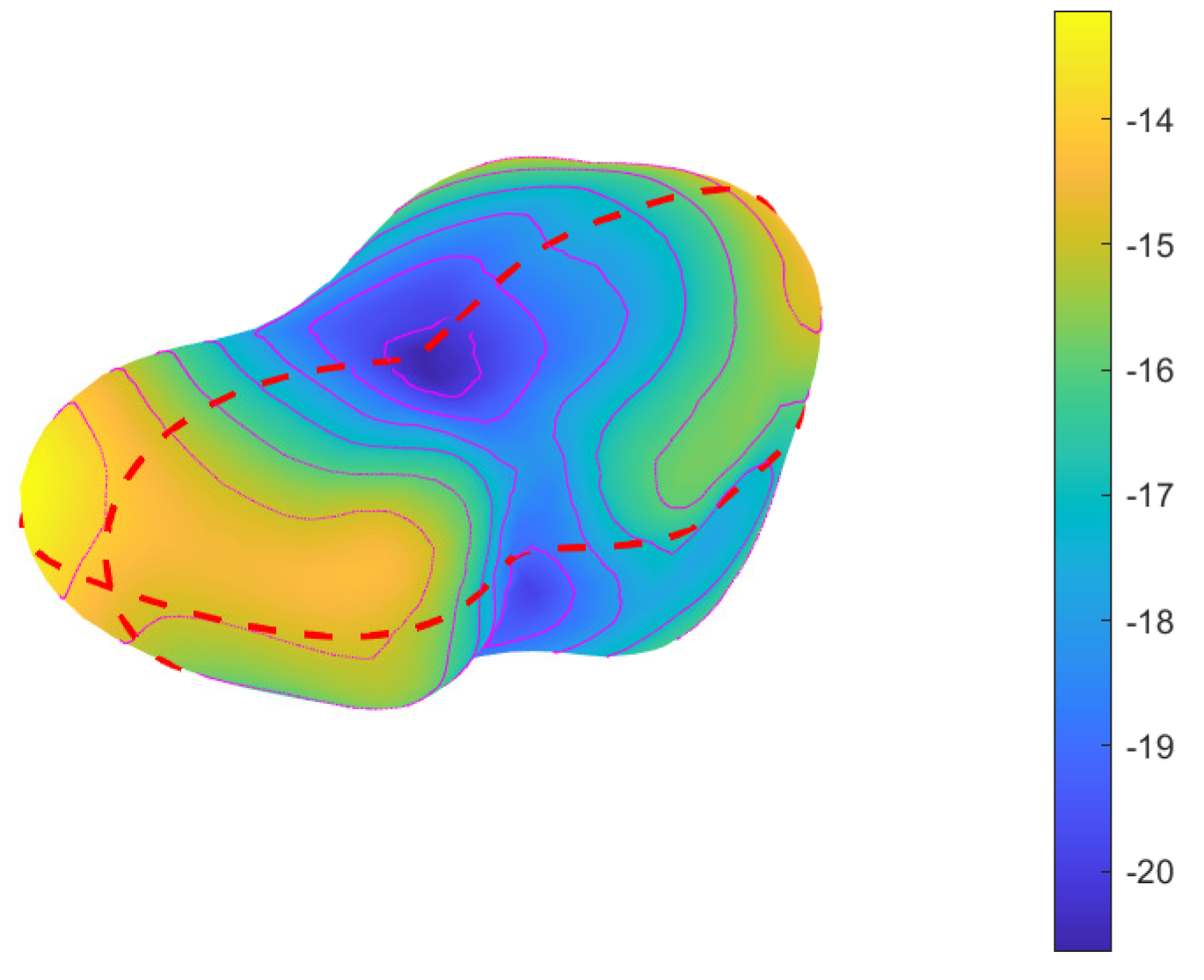
Figure 4.
The contour of the potential, longitude vs. latitude (deg), corresponding to the thin magenta lines in Figure 3. The horizontal red line denotes the plane , i.e., lattitude is zero. And the vertical red dash line denote the palne , i.e., longitudinal is zero.
Figure 4.
The contour of the potential, longitude vs. latitude (deg), corresponding to the thin magenta lines in Figure 3. The horizontal red line denotes the plane , i.e., lattitude is zero. And the vertical red dash line denote the palne , i.e., longitudinal is zero.

Figure 5.
The 3D gravitational acceleration for Castalia on surface. The unit of the color bar is 10 m/s. The red lines are the intercections of the asteroid with its reference sphere whose km.
Figure 5.
The 3D gravitational acceleration for Castalia on surface. The unit of the color bar is 10 m/s. The red lines are the intercections of the asteroid with its reference sphere whose km.

Figure 6.
The contour of the gravitational acceleration. See its corresponding 3D figure, Figure 5. Also, the red lines are the intercections of the asteroid with its reference sphere whose km.
Figure 6.
The contour of the gravitational acceleration. See its corresponding 3D figure, Figure 5. Also, the red lines are the intercections of the asteroid with its reference sphere whose km.
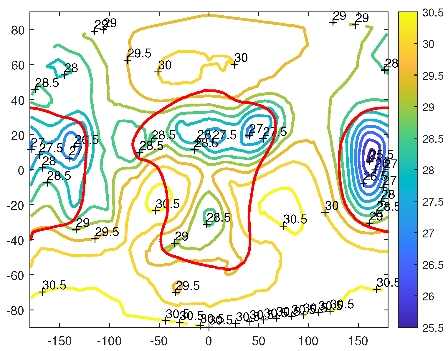
Figure 7.
The gravitational acceleration of the sixth degree and order for Castalia on its surface. The unit of the color bar is 10 m/s.
Figure 7.
The gravitational acceleration of the sixth degree and order for Castalia on its surface. The unit of the color bar is 10 m/s.

Figure 8.
The gravitational acceleration of the 4th degree and order for Castalia on the surface. The unit of the color bar is also 10 m/s.
Figure 8.
The gravitational acceleration of the 4th degree and order for Castalia on the surface. The unit of the color bar is also 10 m/s.

Figure 9.
The gravitational acceleration of the 10th degree and order for Castalia on the surface. The unit of the color bar is also 10 m/s.
Figure 9.
The gravitational acceleration of the 10th degree and order for Castalia on the surface. The unit of the color bar is also 10 m/s.

Figure 10.
The surface tangential acceleration with respect to its gravity horizon when the asteroid does not rotate. The unit of the color bar is 10 m/s.
Figure 10.
The surface tangential acceleration with respect to its gravity horizon when the asteroid does not rotate. The unit of the color bar is 10 m/s.

Figure 11.
The contour map of the surface tangential gravitational acceleration corresponding Figure 10. The unit of the color bar is 10 m/s.
Figure 11.
The contour map of the surface tangential gravitational acceleration corresponding Figure 10. The unit of the color bar is 10 m/s.

Figure 12.
The surface’s effective tangential gravitational acceleration when the asteroid rotates at a period of 4.07 h. The unit of the color bar is 10 m/s.
Figure 12.
The surface’s effective tangential gravitational acceleration when the asteroid rotates at a period of 4.07 h. The unit of the color bar is 10 m/s.

Figure 13.
The contour of the surface’s effective tangential gravitational acceleration corresponding to the 3D Figure 12. The unit of the color bar is also 10 m/s.
Figure 13.
The contour of the surface’s effective tangential gravitational acceleration corresponding to the 3D Figure 12. The unit of the color bar is also 10 m/s.

Figure 14.
The surface’s effective slope when the period is 4.07 h for the asteroid Castalia. Here, the density is 2.1 g/cm. The unit of the color bar is degrees.
Figure 14.
The surface’s effective slope when the period is 4.07 h for the asteroid Castalia. Here, the density is 2.1 g/cm. The unit of the color bar is degrees.

Figure 15.
The 2D contour of the slope, corresponding to Figure 14. The unit of the color bar is degrees.
Figure 15.
The 2D contour of the slope, corresponding to Figure 14. The unit of the color bar is degrees.
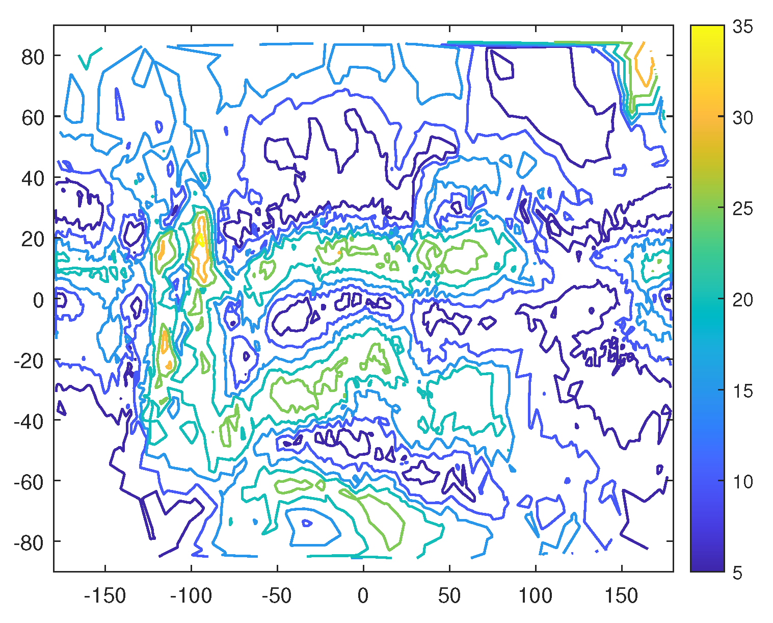
Figure 16.
The histogram of the acceleration slope. Number of faces vs. gravitational slope for the case with rotation (brown) and the case without rotation (blue).
Figure 16.
The histogram of the acceleration slope. Number of faces vs. gravitational slope for the case with rotation (brown) and the case without rotation (blue).

Figure 17.
The gravitational acceleration by polyhedron model at the sphere with an r = 0.5431 km radius. The unit here is 10 m/s. The blue lines is on the surface of the asteroid.
Figure 17.
The gravitational acceleration by polyhedron model at the sphere with an r = 0.5431 km radius. The unit here is 10 m/s. The blue lines is on the surface of the asteroid.

Figure 18.
The corresponding acceleration by the potential of fourth degree and order. The axes are longitude and latitude, respectively.
Figure 18.
The corresponding acceleration by the potential of fourth degree and order. The axes are longitude and latitude, respectively.

Figure 19.
The gravitational acceleration by the polyhedron model at the distance of 2 r sphere. The unit is 10 m/s.
Figure 19.
The gravitational acceleration by the polyhedron model at the distance of 2 r sphere. The unit is 10 m/s.

Figure 20.
The corresponding accelerations by the potential of the 4th degree and order. The axes are longitude and latitude, respectively.
Figure 20.
The corresponding accelerations by the potential of the 4th degree and order. The axes are longitude and latitude, respectively.

Figure 21.
The gravitational acceleration based on the polyhedron model for Castalia at a distance of 3 r. The unit is 10 m/s.
Figure 21.
The gravitational acceleration based on the polyhedron model for Castalia at a distance of 3 r. The unit is 10 m/s.
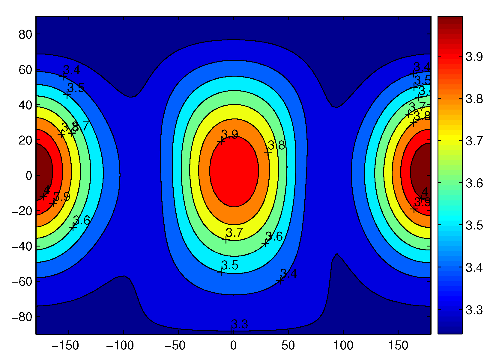
Figure 22.
The corresponding acceleration by the potential of 4 × 4 on the sphere 3 r. The axes are longitude and longitude, respectively.
Figure 22.
The corresponding acceleration by the potential of 4 × 4 on the sphere 3 r. The axes are longitude and longitude, respectively.

Figure 23.
The gravity by the polyhedron model at a distance of 4 r. The unit is 10 m/s.

Figure 24.
Gravity acceleration by the potential of the fourth degree and order on the sphere 4 r. The unit of the color bar is also mgal.
Figure 24.
Gravity acceleration by the potential of the fourth degree and order on the sphere 4 r. The unit of the color bar is also mgal.

Figure 25.
Gravity acceleration based on the 8 × 8 model on the sphere 2 r. The unit here is still mgal = 10 m/s.
Figure 25.
Gravity acceleration based on the 8 × 8 model on the sphere 2 r. The unit here is still mgal = 10 m/s.

Figure 26.
Gravity acceleration based on the 16 × 16 model on a sphere of 2 r. The unit of the color bar is also mgal.
Figure 26.
Gravity acceleration based on the 16 × 16 model on a sphere of 2 r. The unit of the color bar is also mgal.

Figure 27.
The magnitude of gravitational acceleration on the plane without rotation. The unit is 10 m/s.
Figure 27.
The magnitude of gravitational acceleration on the plane without rotation. The unit is 10 m/s.
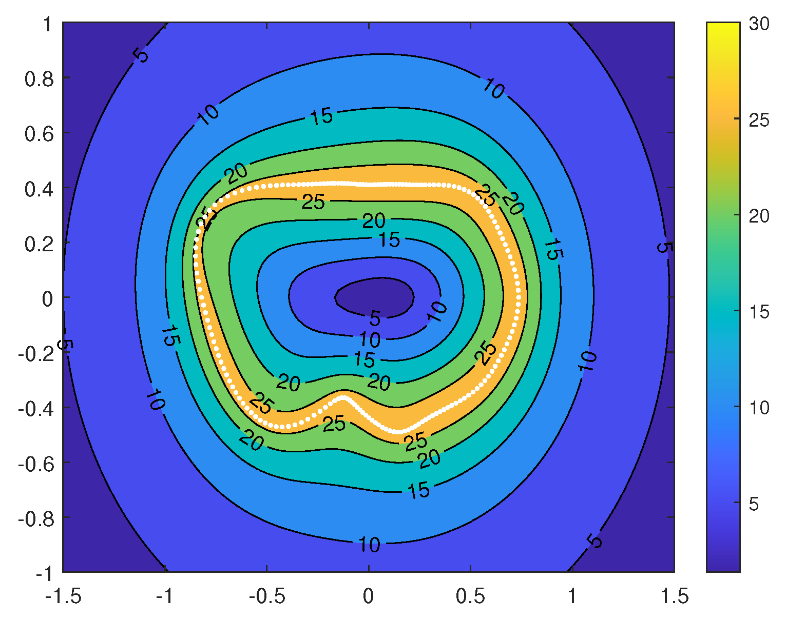
Figure 28.
The effective gravitational acceleration on the plane , when the asteroid rotates with a period of h.
Figure 28.
The effective gravitational acceleration on the plane , when the asteroid rotates with a period of h.

Figure 29.
The effective acceleration direction distribution on the plane , when the asteroid rotates. We can see that all the force inside the astreoid and on the surface, i.e., on the white dashed line, is in the compression direction. There is no force in the tension; i.e., there is no apparent cohesive force for this asteroid. This is a special kind of contribution of this figure. The period is also h. The gravitational values can be seen on the contours in the corresponding figure, Figure 28. The unit of the color bar is 10 m/s.
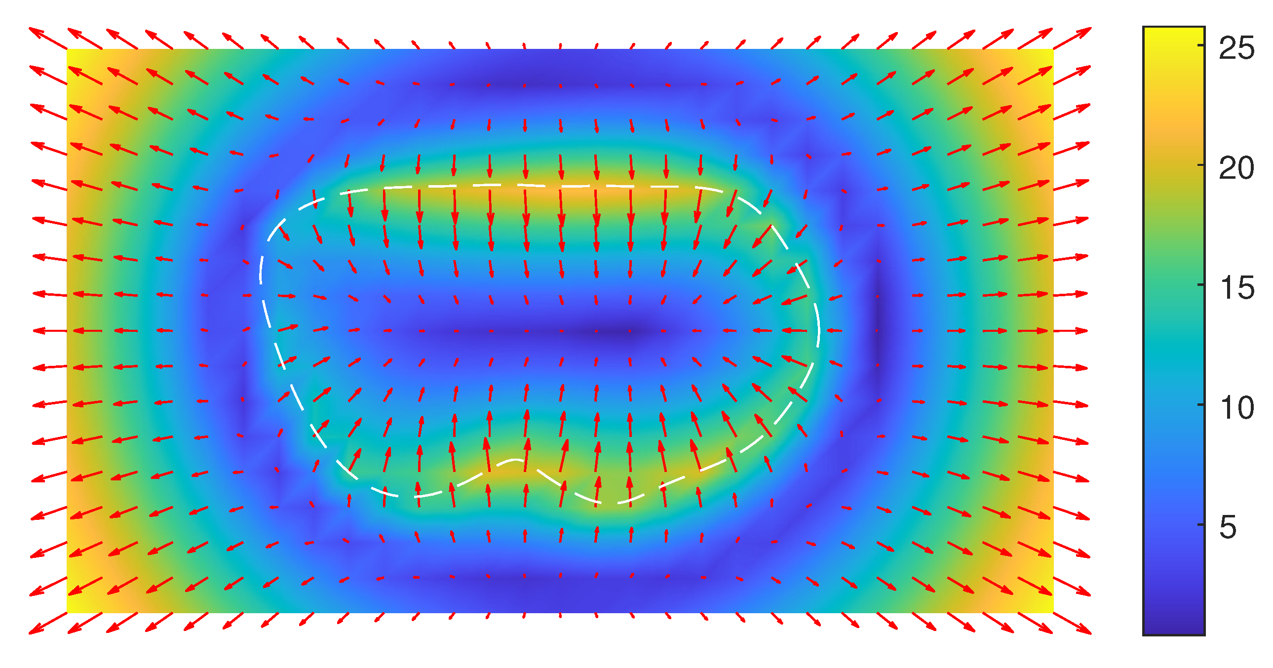
Figure 30.
The gravitational acceleration on the plane without rotation. The unit is 10 m/s.

Figure 31.
The effective gravitational acceleration on the plane when the asteroid rotates.


Table 1.
The spherical harmonic expansion coefficients up to the order and degree of for the asteroid Castalia and a simulated rectangle.
Table 1.
The spherical harmonic expansion coefficients up to the order and degree of for the asteroid Castalia and a simulated rectangle.
| Castalia | Rectangle (1.7 × 0.9 × 0.8) | ||||
|---|---|---|---|---|---|
| n | m | C | S | C | S |
| 0 | 0 | 1.00000000000000 | 0 | 1.000000000000000 | 0 |
| 1 | 0 | −0.00014168122220 | 0 | 0.000000000000000 | 0 |
| 1 | 1 | −0.00004075795821 | −0.00002282770478 | 0.000000000000000 | 0.000000000000000 |
| 2 | 0 | −0.10473883593850 | 0 | −0.102404625451483 | 0 |
| 2 | 1 | 0.00005077855278 | −0.00001641325376 | 0.000000000000000 | 0.000000000000000 |
| 2 | 2 | 0.14774171385537 | −0.00007350942982 | 0.152450260149168 | 0.000000000000000 |
| 3 | 0 | −0.01992884455238 | 0 | 0.000000000000000 | 0 |
| 3 | 1 | −0.03410426627931 | 0.00074227942951 | 0.000000000000000 | 0.000000000000000 |
| 3 | 2 | 0.01165825781331 | 0.00224122654733 | 0.000000000000000 | 0.000000000000000 |
| 3 | 3 | 0.01771996117460 | −0.01186045941413 | 0.000000000000000 | 0.000000000000000 |
| 4 | 0 | 0.03510656662646 | 0 | 0.017542426440102 | 0 |
| 4 | 1 | 0.00260220108679 | 0.00163584922657 | 0.000000000000000 | 0.000000000000000 |
| 4 | 2 | −0.04830939903696 | 0.00311423803618 | −0.039143149995087 | 0.000000000000000 |
| 4 | 3 | 0.00690976107455 | −0.00383406677217 | 0.000000000000000 | 0.000000000000000 |
| 4 | 4 | 0.04473930002048 | −0.01216108958396 | 0.019151577641493 | 0.000000000000000 |
| 5 | 0 | 0.02398903330765 | 0 | 0.000000000000000 | 0.000000000000000 |
| 5 | 1 | 0.03681372375277 | −0.00231269356380 | 0.000000000000000 | 0.000000000000000 |
| 5 | 2 | −0.02285422699738 | −0.00181873143701 | 0.000000000000000 | 0.000000000000000 |
| 5 | 3 | −0.02349704830265 | 0.00997187133947 | 0.000000000000000 | 0.000000000000000 |
| 5 | 4 | 0.00652991532599 | −0.00084721036230 | 0.000000000000000 | 0.000000000000000 |
| 5 | 5 | 0.00353895156596 | −0.02436464043876 | 0.000000000000000 | 0.000000000000000 |
| 6 | 0 | −0.01499101017996 | 0 | 0.021480381809402 | 0 |
| 6 | 1 | 0.00183803644113 | −0.00116294838910 | 0.000000000000000 | 0.000000000000000 |
| 6 | 2 | 0.02197171243552 | −0.00529808274697 | −0.014894515446723 | 0.000000000000000 |
| 6 | 3 | −0.00577570989586 | 0.00446161579351 | 0.000000000000000 | 0.000000000000000 |
| 6 | 4 | −0.01904232642471 | 0.01127642233858 | −0.003093652246108 | 0.000000000000000 |
| 6 | 5 | 0.00690519883075 | −0.00499919673362 | 0.000000000000000 | 0.000000000000000 |
| 6 | 6 | 0.01326276839505 | −0.02937007076311 | −0.051021169584544 | 0.000000000000000 |
Disclaimer/Publisher’s Note: The statements, opinions and data contained in all publications are solely those of the individual author(s) and contributor(s) and not of MDPI and/or the editor(s). MDPI and/or the editor(s) disclaim responsibility for any injury to people or property resulting from any ideas, methods, instructions or products referred to in the content. |
© 2024 by the authors. Licensee MDPI, Basel, Switzerland. This article is an open access article distributed under the terms and conditions of the Creative Commons Attribution (CC BY) license (https://creativecommons.org/licenses/by/4.0/).
Share and Cite
MDPI and ACS Style
Hu, W.; Fu, T.; Liu, C. Revisiting the Numerical Evaluation and Visualization of the Gravity Fields of Asteroid 4769 Castalia Using Polyhedron and Harmonic Expansions Models. Appl. Sci. 2024, 14, 4058. https://doi.org/10.3390/app14104058
AMA Style
Hu W, Fu T, Liu C. Revisiting the Numerical Evaluation and Visualization of the Gravity Fields of Asteroid 4769 Castalia Using Polyhedron and Harmonic Expansions Models. Applied Sciences. 2024; 14(10):4058. https://doi.org/10.3390/app14104058
Chicago/Turabian StyleHu, Weiduo, Tao Fu, and Chang Liu. 2024. "Revisiting the Numerical Evaluation and Visualization of the Gravity Fields of Asteroid 4769 Castalia Using Polyhedron and Harmonic Expansions Models" Applied Sciences 14, no. 10: 4058. https://doi.org/10.3390/app14104058
Note that from the first issue of 2016, this journal uses article numbers instead of page numbers. See further details here.