Analyzing the Impact of Geometrophysical Modeling on Highway Design Speeds: A Comparative Study for Mexico’s Case

Abstract

This manuscript presents an examination of the impact of geometrical and physical parameters on highway design speeds, critical for traffic safety and efficiency. Originating from a classical dynamics discussion in an undergraduate automotive technology engineering class, an exploration of the consequences of different geometrophysical considerations on a vehicle’s dynamics over pavement surfaces is developed. Considering various analytical models, an assessment of their principles and the significance of geometric and physical concepts involved in the problem is made, such as plane of motion and trajectory curvature radius, on safe (non slippage) operational speeds. The subsequent comparative study shows that one of the most accepted models in highway design regulations in México, when used as reference, yields percentage error differences respect to others of $0\lesssim \%E_{Max}\lesssim 5$, as well as a consistent trend for relatively underestimating safe highway operational speeds. A discussion of the immediate implications of these findings, emphasizing the necessity of experimental studies to validate theoretical predictions, is presented. This work contributes to the field by providing a detailed comparison of analytical models under a general applied science perspective, suggesting modifications to current highway design practices in México based on geometrophysical insights. In summary, this work’s main aim is to shed light on the intricacies of determining safe design speeds from an applied sciences point of view, while also calling for a reevaluation of the existing guidelines to enhance highway design and safety.

1. Introduction and Antecedents

Highway design significantly impacts traffic safety and efficiency, with a focus on establishing safe, practical operational speeds. The research on the interplay between design speed and highway safety seeks to formulate supportive guidelines and models for informed highway design. This section first synthesizes the academic findings on safe design traffic speeds, encompassing six critical areas.

Predictive structural modeling and analysis. The recent studies have highlighted the importance of integrating advanced structural dynamics and stress-response analyses into highway design. Among them are studies on the structural resistance of reinforced concrete columns and circular hollow section (CHS) joints under bending moments, in which neural network modeling and BP-Garson algorithmization are used to predict and analyze critical structural behaviors, which clearly is directly applicable to highway design and its operational safety and integrity [1]. On the other hand, studies in subjects such as the analysis of the effects of the brace-to-chord angle on the capacity of multi-planar CHS X-joints under out-of-plane bending moments illustrate how spatial and angular factors, modeled through finite element analysis, influence structural capacity, which is critical in highway design [2].

Operating Speed Prediction Models. The quest for design consistency has propelled the development of models to predict operating speeds, based on driver behavior analysis. The recent advances utilize dynamic-driving simulators to capture continuous speed profiles, offering deeper insights into driver behaviors on various roadway configurations [3].

Effects of Changing Highway Design Speed. Evaluating the implications of design speed adjustments through surveys and case studies has shed light on design engineers’ perspectives and the consequential shifts in traffic dynamics, notably in traffic flow, speed patterns, and accident rates [4].

Driver Errors on Highway Segments. Acknowledging driver errors as a fundamental concern in highway safety means this area integrates human factors into roadway guidelines, emphasizing the necessity of understanding the underlying causes of errors for the design of safer roadways and the implementation of effective traffic management [5].

Acceleration Lengths for Entrance Terminals. The critical analysis of entrance ramp acceleration lengths suggests a potential revision of the existing standards to improve traffic integration and reduce collision risks, highlighting the importance of infrastructure adaptability to driving behaviors [6].

Design Speeds and Speed Limits. Design speeds play a crucial role in ensuring safe highway operations. Highways should be designed in a conservative manner to accommodate the speed that drivers are likely to develop. However, actual freeflow speeds may exceed the design speed, and this situation does not necessarily lead to excessive hazards if drivers adequately perceive the risks involved. Ensuring consistency between design speeds and speed limits is, therefore, essential for promoting safe and efficient traffic flow [7].

Therefore, the academic research on safe design traffic speed on highways has made contributions to understanding the relationship between design speed and highway safety. Apart from the perspectives mentioned in the previous paragraphs, studies have also investigated operating speed prediction models, the effects of changing design speed, driver errors, acceleration lengths, and the relationship between design speeds and speed limits. These findings provide valuable insights for highway designers, engineers, and policymakers in developing guidelines and strategies to enhance highway safety and efficiency. Complementarily, this paper focuses on the role of geometrophysical parameters such as super-elevation rate and curvature radius over maximum safe speeds in highways, further exploring their influence on vehicle dynamics and their implications for highway policy and safety measures [8,9,10,11]. That relates to the last bullet point in the previous paragraphs.

However, we find that many of these studies rely on one perhaps unnoticed applied conceptual framework of classical dynamics, which could hinder practical considerations related to highway design, construction, and operation. It is, in our perception, a subject of considering the critical aspects of the same problem from different perspectives. This conceptual framework is referred to here as the instantaneous radius of curvature model (IRCM) for highway vehicle dynamics. One of its main characteristics is its wide use when defining the trajectory of a vehicle on the pavement [12,13,14,15]. More details are found in Section 3.1. We posit that the problem can also be analyzed in terms of alternative geometric–physical parameters, opening unconsidered perspectives for assessing highway planning, building, and safe operation. Nevertheless, the detailed development of those remains the matter of future studies. In particular, several simple geometrical models in which the problem of a moving vehicle’s basic dynamics on a super-elevated pavement can be analyzed with the IRCM model were considered, as well as others applicable to the basic geometrophysical formulation of the problem. Those results are compared, and subsequently, the points of interest in related subjects are briefly discussed.

This paper is organized as follows: a first section presents introductory remarks and general context. It is followed by a second section attempting to provide context into what is meant in this work by geometrophysical modeling. In the third, several different geometrophysical models are set up and discussed to obtain safe highway operating speeds according to each one. In the fourth, the results from the models are presented and compared using parameters found in the literature applicable to the Mexican case. In the fifth section, those results are discussed. Finally, a sixth one is submitted with conclusive comments. This way, an applied science exploration of geometrophysical models for safe operating highway speeds leads to a conclusive comparative analysis using Mexican parameters and regulative framework.

2. A Brief Comment on Geometrophysical Modeling

Geometrophysical modeling is, in the context of the present work, a sophisticated applied sciences analytical approach that integrates principles of geometry and physics to solve complex problems in various engineering fields, including highway engineering. This section seeks to briefly present some of the core concepts and general methodological principles employed in geometrophysical modeling, enhancing the reader’s understanding of its application related to this work, i.e., the assessment and development of highway regulations in Mexico.

2.1. Fundamental Principles

At its core, geometrophysical modeling involves the use of geometric principles/data, such as shapes, sizes, and relative positions of objects, combined with the physical laws governing the dynamics of those objects under study. For highway engineering, these principles are applied to understand and predict the behavior of vehicles under different road conditions and configurations. The models considered are developed in Section 3.

2.2. Modeling Dynamics

The models discussed in this manuscript are derived from classical dynamics principles. These dictate how vehicles move and interact based on physical parameters such as momentum, friction, highway plane inclination with respect to the ground, and gravity. Of particular interest to this present work are the maximum non-slippage speeds predicted by the models, since they would represent maximum design safe speed estimations in highway engineering. The models considered are discussed in Section 4.

2.3. Application to Highway Regulations

Regarding highway regulations, geometrophysical models can be used to optimize road design, improve safety standards, and enhance traffic flow efficiency. By applying these models, engineers can determine the optimal curvature of roads that balances safety and speed or establish speed limits that are based on the physical capabilities of the road and typical vehicle performances. One application example related to modeling accidents and highway geometric design relationships is found in [16]. In that study, the capabilities and limitations of regression models are explored to help understand the relationships between vehicle accidents and highway geometric design, emphasizing the need to develop proper statistical models to handle the variability and distribution of accident data. In [17], there is another application example. This study discusses the impact that geometric design characteristics have on traffic safety. Statistical negative binomial regression modeling is used to better understand factors related to highway geometric influencing accident frequency, identifying operating speeds (the central parameter in this present study) as one of the main factors contributing to the total number of accidents. These examples, among others, illustrate how geometrophysical considerations can contribute to a better understanding of how modeling and design factors are linked to regulatory outcomes and safety on highways.

2.4. Comparative Analysis

This manuscript compares various geometrophysical models to identify which configurations best meet the regulatory standards and practical needs of Mexican highways, having the reference model expressed by Equation (14) (please Cf. [18]). Generally speaking, the models could be evaluated based on several metrics, such as safety, cost-effectiveness, and environmental impact. In the case of this present work, the metric used was the maximum design non-slippage velocity, i.e., the safe velocity on the highway under consideration. This analysis (Cf. Section 4 and Section 5) is crucial for policymakers and engineers to make informed decisions about which models to implement in practice.

2.5. Relevance of Geometrophysical Modeling/Examples

Understanding geometrophysical modeling is essential for anyone involved in the planning, design, or regulation of highways. It provides a scientific basis for making decisions affecting the safety and functionality of road systems, ensuring that these infrastructures can accommodate the current and future transportation needs effectively. Here there are some examples. Albattah (2016) uses spatial satellite remote sensing data integrated with geographic information system (GIS) models to optimize highway design in [19]. It includes factors like land use, geology, and environmental impacts to select the best route corridor for minimizing costs and conforming to environmental requirements. Boas et al. (2009) modeled highway systems using a modified geometrical network model, integrating paths instead of edges for optimal parameter configurations, and comparing models from different countries in [20]. In another example, Biancardo et al. (2020) explore the integration of building information modeling (BIM) with procedural modeling tools for road infrastructure, focusing on geometric and physical aspects. The use of BIM for complex road design is highlighted, enhancing data interoperability and management of geometric properties critical for transportation infrastructure in smart urban environments [21]. Wang et al. (2023) introduce a framework intended to enhance geometric information extraction and digital modeling from LiDAR data, targeting road scenarios. This approach addresses the challenge of handling unorganized point clouds and complex environments, demonstrating high accuracy in semantic segmentation and geometric precision, which is crucial for practical applications in road engineering [22]. Qi et al. (2023) present a method for three-dimensional fine modeling of in-service roads using vehicle laser scanning technology. It focuses on multi-level reverse modeling based on point cloud data, offering a structured approach to reduce data redundancy and enhance model accuracy. The method supports various levels of detail (LOD), allowing for tailored model fineness and application-specific accuracy, which proves effective in managing complex road infrastructures [23]. Wei et al. (2023) present an innovative approach for simultaneous multi-curve highway reconstruction from mobile laser scanning data, leveraging deep reinforcement learning with the proximal policy optimization algorithm. This method allows for the effective geometric modeling of complex highway curves, demonstrating superior performance in capturing accurate road configurations compared to the previous techniques [24]. These papers provide a range of instances related to geometrophysical modeling applied to the context of roads and highway engineering, highlighting advancements such as GIS integration, 3D geometric modeling, and network optimization in transportation planning.

3. Analytical Model Conceptual Development and Discussion

In this section, details on developing the analytical models to assess the simplified dynamics of a four-rubber-wheeled vehicle on the pavement are provided. Most of the geometrophysical models to be discussed are common knowledge in the literature. However, our interest centers on their conceptual setting up, discussion, and interpretation from a geometrophysical perspective, which has been not carried out to the extent of our knowledge. This way, we can search for insights regarding their application in highway design, construction, and operation. As mentioned, the problem consists of analyzing forces acting on a vehicle supported by rubber wheels while in motion over the pavement. For simplicity, highways are considered single slope cambered with a super-elevation angle (Cf. Figure 1, and then Figure 2). The majority of curves anticipated in the design of the layout of a highway are of this type. Furthermore, this is the strategy adopted by AASHTO when proposing the foundations of the analysis of safe speeds in curves in [25]. Furthermore, the problem is considered to be a single particle dynamics one, i.e., the vehicle is represented entirely by its center of gravity. However, that does not imply critical loss of generality, since particular interest centers on the role of super-elevation rate, curvature radius, and other parameters similar to the latter intervening in vehicle behavior and highway operation.

3.1. Instantaneous Radius of Curvature Model (IRCM) for Highway Vehicle Dynamics: Normal and Tangential Coordinates

Motion is considered on a plane with two coordinates, one normal or perpendicular to the trajectory and another tangential or parallel. Mathematically, this model could be assimilated to the 2D motion studied via polar coordinates (not cylindrical-polar 3D ones). The radial coordinate would be the one normal to the trajectory, and the angular coordinate the one tangential to it, as depicted in Figure 1. It should be noticed that conceptually speaking, this model, or slight variations on it, is the one most governmental-associated regulators use to provide highway design criteria and is based, as mentioned, on a point-mass dynamics consideration of the problem combined with the criterion of favoring driver comfort [8,9]. Particularly, authorities such as FRA, AREMA, Amtrak, and OSHA set $0.1g[m/s^2]$ and $0.03g[s^{-1}$] − $[m/s^3]$ as maximum acceptable values for radial/normal acceleration and jerk, respectively [13,25,26]. The model gives the following result, called the basic curve equation Cf. [25]:

$$\begin{array}{c}\hfill v=\sqrt{\frac{127R(f_d+0.01e)}{1.0-0.01e{f}_d}}\end{array}$$

(1)

In it, v is the design speed in $[km/h]$, $f_d$ is the estimated side friction demand factor, R is the horizontal curve radius in $\left[m\right]$, and e is the super-elevation in % ratio. In order to compare this model to others, friction must be taken into account as a free parameter (subjected to applicable physical restrictions) instead of as a parameter according to the driver’s comfortable acceleration friction demand term ($f_d$). On the other hand, in highway design, it is customary to consider the product $e{f}_d$ invariably as very small, so the term $1.0-0.01e{f}_d\simeq 1.0$ (Cf. [25]). This way, the basic curve equation turns into

$$\begin{array}{c}\hfill v=\sqrt{127R(f_d+0.01e)}\end{array}$$

(2)

In the case of this manuscript, the model is discussed from principles in the following lines.

The kinematics/dynamics analysis begins by considering the following expressions:

$$\begin{array}{cc}\hfill \overrightarrow{v}& =v\widehat{\theta }\hfill \\ \hfill \overrightarrow{a}& =\dot{\overrightarrow{v}}=\dot{v}\widehat{\theta }+v\dot{\widehat{\theta }}\hfill \end{array}$$

(3)

Resulting in

$$\overrightarrow{a}=a_r\widehat{r}+a_{\theta }\widehat{\theta }=-\frac{v^2}{r}\widehat{r}+\dot{v}\widehat{\theta }$$

(4)

Therefore, the velocity direction is tangent to the motion’s trajectory and has only that component. In contrast, acceleration has both normal (in the direction of $\widehat{r}$) and tangential (in the direction of $\widehat{\theta }$) components. Now, normal acceleration magnitude is the vehicle’s speed squared divided by the trajectory’s curvature radius, which, at the same time, is the vehicle’s radial coordinate magnitude ($v^2/r$). In turn, tangential acceleration magnitude is the time derivative of the coordinate along the line of motion ($\dot{v}$).

Figure 1. Diagram of the normal and tangential coordinates geometric setup used to define and develop the instantaneous radius of curvature 2D model IRCM for highway vehicle dynamics. In this figure, r is the trajectory’s curvature radius and, simultaneously, the radial coordinate (in the cylindrical-polar coordinate system), $\theta$ is the vehicle’s instantaneous angular position/polar coordinate (in the cylindrical-polar coordinate system), and $\widehat{x}$, $\widehat{y}$ are the 2D Cartesian coordinate system unit vectors.

Figure 1. Diagram of the normal and tangential coordinates geometric setup used to define and develop the instantaneous radius of curvature 2D model IRCM for highway vehicle dynamics. In this figure, r is the trajectory’s curvature radius and, simultaneously, the radial coordinate (in the cylindrical-polar coordinate system), $\theta$ is the vehicle’s instantaneous angular position/polar coordinate (in the cylindrical-polar coordinate system), and $\widehat{x}$, $\widehat{y}$ are the 2D Cartesian coordinate system unit vectors.

Applying the preceding model features to the layout presented by Figure 2, it is noticeable that even though the problem is 3D, the model emphasizes consideration of 2D motion on the plane defined by those normal and tangential coordinates; therefore, adjustments must be conducted, as is shown. It is also noticeable that the “normal” coordinate coincides with the regular Cartesian $\widehat{x}$ coordinate, and “tangential” coordinate, corresponds to regular Cartesian $\widehat{z}$ coordinate. That is, the last coordinate coming out of the plane of the page towards the reader is consistent with a right-handed Cartesian coordinate system.

Figure 2. General layout of the problem’s dynamic and the geometrophysical scheme applied to account for it. The model uses “normal”, y, and “tangential” coordinates; that is, ($x;y;z$). In this figure, $\overrightarrow{N}$, $\overrightarrow{F}$, $\overrightarrow{W}$ are the forces acting on the vehicle: normal, friction, and weight; respectively. The angle $\theta$ is the highway’s considered super-elevation. $\widehat{x}$, $\widehat{y}$, $\widehat{z}$ are the 3D Cartesian coordinate system unit vectors.

Figure 2. General layout of the problem’s dynamic and the geometrophysical scheme applied to account for it. The model uses “normal”, y, and “tangential” coordinates; that is, ($x;y;z$). In this figure, $\overrightarrow{N}$, $\overrightarrow{F}$, $\overrightarrow{W}$ are the forces acting on the vehicle: normal, friction, and weight; respectively. The angle $\theta$ is the highway’s considered super-elevation. $\widehat{x}$, $\widehat{y}$, $\widehat{z}$ are the 3D Cartesian coordinate system unit vectors.

Considering an instantaneous validity of the dynamic situation as shown in Figure 2, the application of the second law of Newton on the vehicle results in:

$$\overrightarrow{N}+\overrightarrow{W}+\overrightarrow{F}=m\overrightarrow{a}$$

(5)

$\overrightarrow{N}$ is the normal force exerted by the surface of the highway on the vehicle, $\overrightarrow{W}$ is the weight of the vehicle, $\overrightarrow{F}$ is the friction force applied by the surface of the highway on the vehicle, m is the vehicle’s mass, and $\overrightarrow{a}$ is its acceleration. In Cartesian—$\widehat{i},\widehat{j},\widehat{k}$—component vector representation, Equation (5) yields

$$\begin{array}{c}\hfill \left(-Nsin\theta ;Ncos\theta ;0\right)+\left(0;-mg;0\right)+\left(-\mu Ncos\theta ;-\mu Nsin\theta ;0\right)\\ \hfill =m\left(-v^2/R;0;0\right)\end{array}$$

(6)

$\theta$ is the highway super-elevation angle, g is the gravitational acceleration magnitude, $\mu$ is the friction coefficient between the vehicle’s tires and pavement, v is the vehicle’s speed at which the system is in dynamic equilibrium, and R is its instantaneous trajectory curvature radius. The minus sign on the first term after the equal sign in Equation (6) means that for the dynamical equilibrium situation considered, the normal component of the vehicle’s acceleration is centripetal, because it represents the force equilibrating the non-kinetic friction force between the vehicle tires and pavement (i.e., $\overrightarrow{F}$ in Equation (5)). At any given time, the vehicle’s trajectory places it at a point on the circle described in the $x-z$ plane of Figure 2. Then, it is vital to notice that the trajectory plane is not parallel to the inclined plane of the pavement in Figure 2. A visual scheme of precisely that “trajectory” is provided in Figure 3. On the other hand, the validity of the instantaneous dynamic situation portrayed in Figure 2 means that v in Equation (6) corresponds to the case in which there is no drift between the vehicle’s tires and pavement. This means that when solving for v, the system of scalar equations provided by vector Equation (6) provides us with the maximum speed value permitted by a given highway at which the vehicle is in dynamic equilibrium along it with no drift. That is the maximum velocity for safe highway operation. The solution for v is as follows:

$$v=\sqrt{\frac{gR\left(sin\theta +\mu cos\theta \right)}{cos\theta -\mu sin\theta }}=\sqrt{\frac{gR\left(\mu +tan\theta \right)}{1-\mu tan\theta }}$$

(7)

In order for this model application to be meaningful regarding highway design (particularly on the physical and engineering meaningfulness of the curvature radius parameter R), one has to take into account the following:

(i)

A 2D model is used to ascertain a 3D situation. The motion of a vehicle on the highway can not be reduced to normal and tangential components. For the model to make sense, another coordinate along $\widehat{y}$ is used.

(ii)

A radius of the curvature (R) notion only makes sense when considering sequences of precise segments of circular/curvilinear sections; that is, definite arc segments of the vehicle’s trajectory, as shown in Figure 3.

(iii)

Equations (1) and (7) (right) are functionally equivalent since they both are the results of point mass modeling considerations. It can be noticed that Equation (1) is a reparametrization of Equation (7) (right), performed by AASHTO in [25].

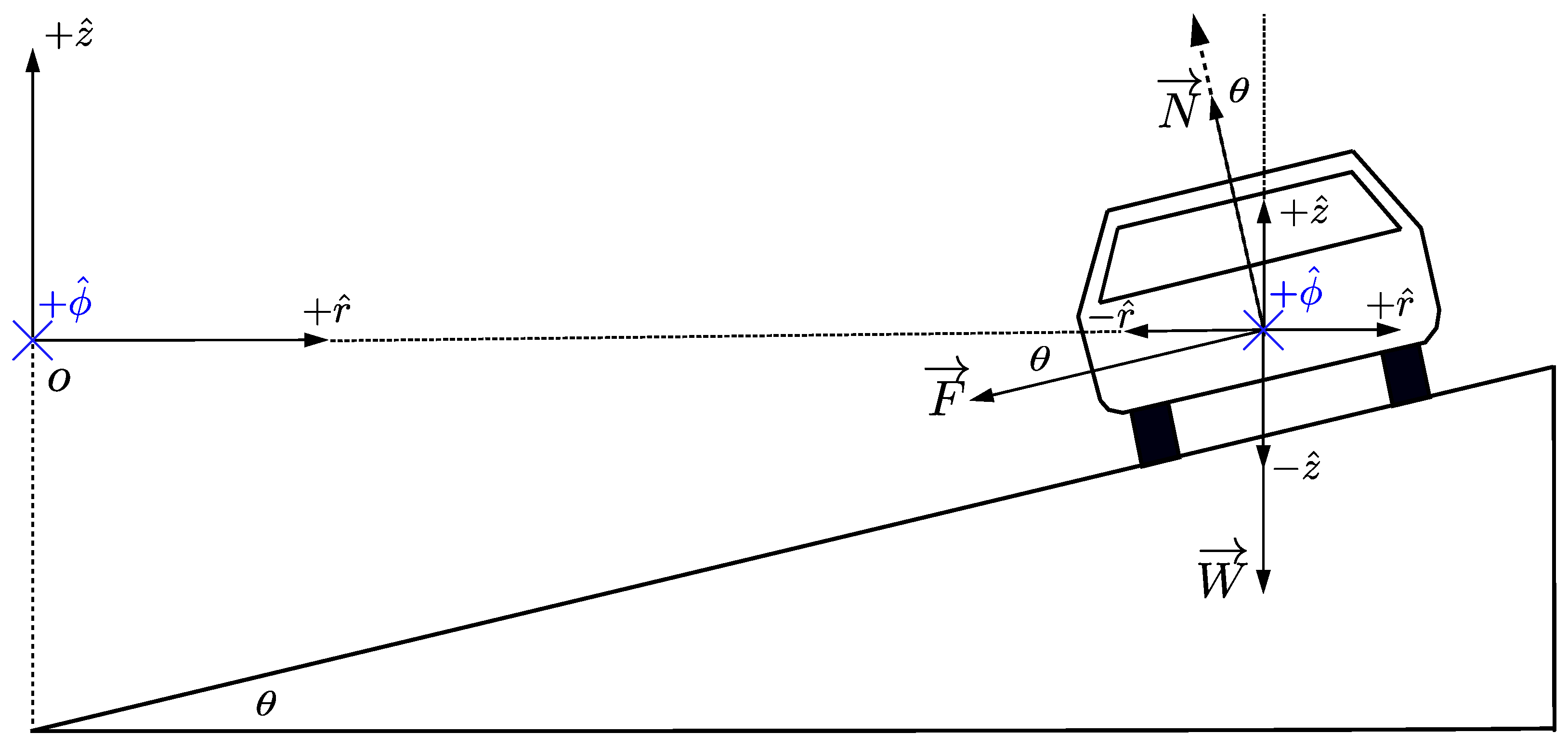
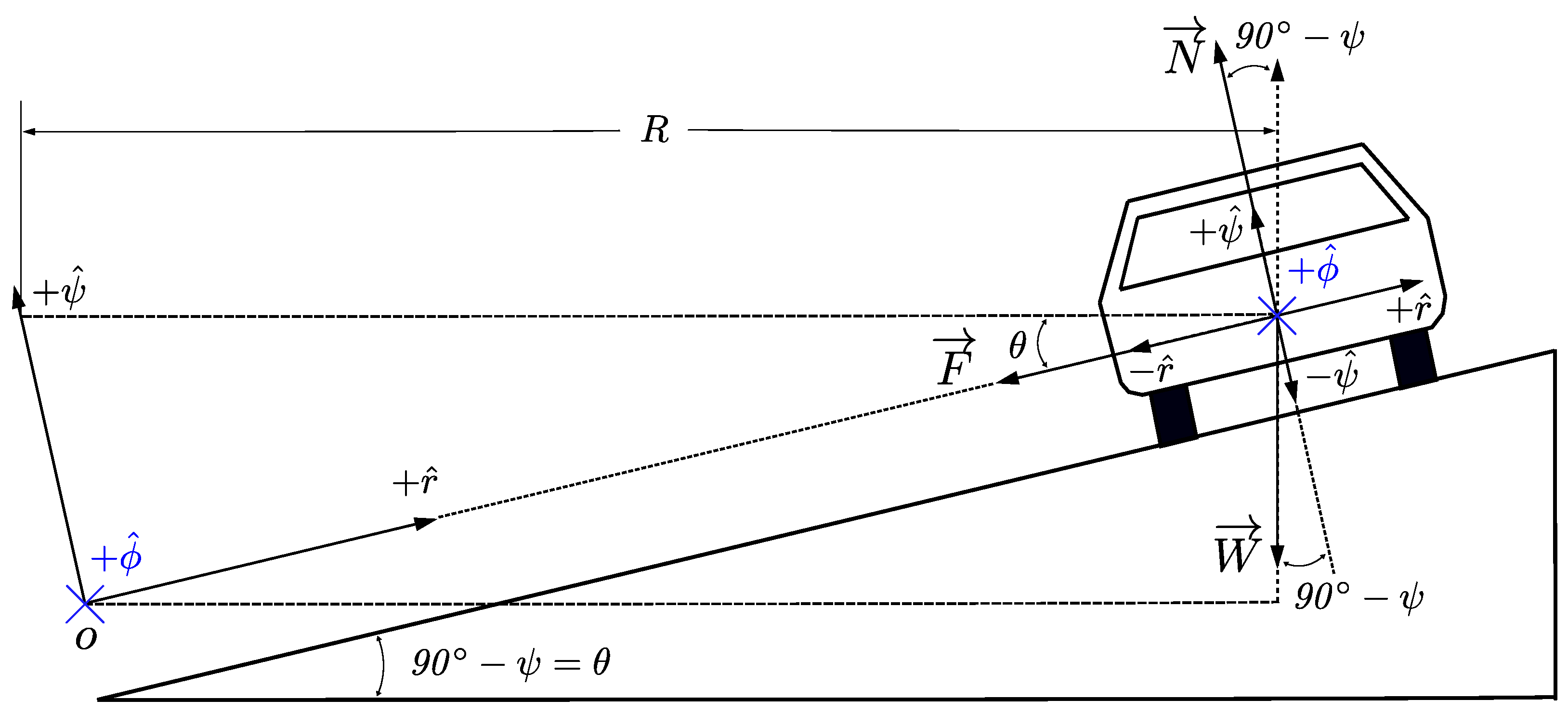
3.2. Highway Vehicle Dynamics Studied by Cylindrical-Polar Coordinates: Plane of Vehicle Motion Rotated with Respect to Horizontal Plane

The situation is reviewed with cylindrical-polar coordinates, as shown in Figure 4. This way, one would have two coordinates normal to the motion’s trajectory, r and z, and one tangential ($\varphi$). As is noticeable in the figure, the $\varphi$ coordinate’s unit vector goes into (i.e., enters) the page’s plane. This way, r, $\varphi$, and z set up an orthonormal coordinate system.

On the other hand, the main difference between the models in Figure 2 and Figure 4 is that the plane of the circular trajectory in the former is unrotated with respect to the x axis, while in the latter, it is rotated by an amount of $\theta$, the highway super-elevation parameter. In other words, the vehicle’s trajectory is the same as shown in Figure 3 but with its plane parallel to the pavement’s plane, as portrayed in Figure 4. Both possibilities are reasonable since, as said, the dynamic situation is considered to be instantaneous without a critical loss of generality. In practice, the vehicle is neither expected to fulfill the trajectories envisioned by Figure 2 or Figure 4. In this system, the position vector is as follows in terms of Cartesian unit vectors:

$$\overrightarrow{r}=rcos\varphi \widehat{i}+rsin\varphi \widehat{j}+z\widehat{k}$$

(8)

The calculation of the second derivative of $\overrightarrow{r}$, i.e., acceleration ($\overrightarrow{a}$), yields

$$\begin{array}{cc}\hfill & \overrightarrow{a}=\left(cos\varphi (\ddot{r}-r{\dot{\varphi }}^2)-sin\varphi (r\ddot{\varphi }+2\dot{r}\dot{\varphi })\right)\widehat{i}\hfill \\ \hfill & +\left(sin\varphi (\ddot{r}-r{\dot{\varphi }}^2)+rcos\varphi \ddot{\varphi }+2cos\varphi \dot{r}\dot{\varphi }\right)\widehat{j}+\ddot{z}\widehat{k}\hfill \end{array}$$

(9)

The particular conditions of the model to implement are $\dot{r}=0$, $\ddot{r}=0$, $\ddot{\varphi }=0$, $\dot{z}=0$, and $\ddot{z}=0$, since within the dynamic situation considered, there is no velocity or acceleration along radial and z coordinates. Meanwhile, for the angular coordinate, there is no acceleration. These considerations in Equation (9) lead us to

$$\overrightarrow{a}=-rcos\varphi {\dot{\varphi }}^2\widehat{i}-rsin\varphi {\dot{\varphi }}^2\widehat{j}+0\widehat{k}$$

(10)

Or, in cylindrical-polar component vector representation, $\widehat{r},\widehat{\varphi },\widehat{z}$,

$$\overrightarrow{a}=-r{\dot{\varphi }}^2\widehat{r}+0\widehat{\varphi }+0\widehat{z}$$

(11)

Now, Equation (5) applied to the situation in Figure 4, and taking into account Equation (11), yields, in cylindrical-polar component vector representation, $\widehat{r},\widehat{\varphi },\widehat{z}$,

$$\begin{array}{c}\hfill \left(0;0;N\right)+\left(-mgsin\theta ;0;-mgcos\theta \right)+\left(-\mu N;0;0\right)\\ \hfill =m\left(-v^2/r;0;0\right)\end{array}$$

(12)

where $v=r\dot{\varphi }$. In this case, r is both an instantaneous radius of curvature of the vehicle’s trajectory, as well as the radial coordinate of the system used to analyze the problem. Solving for v in Equation (11) produces, as before in Equation (7), the maximum velocity for safe highway operation according to the model:

$$v=\sqrt{grcos\theta \left(tan\theta +\mu \right)}=\sqrt{gr(sin\theta +\mu cos\theta )}$$

(13)

In terms of the radius of curvature ($R=rcos\theta$) Cf. Figure 4. Equation (13) right transforms into

$$v=\sqrt{gR(\mu +tan\theta )}$$

(14)

Now the models in Equations (2) and (14) can be compared. In the former, $f_d(v,R,e)=\frac{v^2}{k_{1}R}-k_{2}e$ is defined as the amount of friction a vehicle needs in order to maintain trajectory in an existing horizontal curve [26]. On the other hand, $k_1$ and $k_2$ are parameters considering the suspension’s mechanical effect on light and heavy vehicles, respectively. It is noticeable that Equations (2) and (14) share the same analytical elements, both having the mathematical form $v=\sqrt{c_1(c_2+c_3)}$. In this equation form, $c_1\Rightarrow 15R\Rightarrow gR$ relates to the motion’s curvature radius, $c_2\Rightarrow f_d\Rightarrow \mu$ relates to friction, and $c_3\Rightarrow 0.01e\Rightarrow tan\theta$ relates to the highway’s super-elevation, respectively. Another point of comparison between models is that Equations (2) and (14) both take into account the instantaneous friction being provided by horizontal curves in the trajectory. Cf. [26] or friction demand ($f_d$) definition; see Figure 4 here for friction force ($\overrightarrow{F}$) consideration. For these reasons, Equation (14) is selected as the reference for comparison between models.

Summarizing this last part, the model according to Equation (14) is selected as reference for comparison to the others because it was shown that it amounts to a reparametrization of the one in Equation (2), which happens to be the one used as the base in Mexico’s regulations (Manual de proyecto geométrico de carreteras 2018—Handbook of geometric projects in highways 2018) [18]. On the other hand, the percentages of relative error differences among safe (i.e., non slippage) highway design speeds generated by models considered with respect to the one generated by Equation (14) are proposed as suitable comparison metrics between them. Those differences are analytically interesting since they can be directly interpreted as potential errors in highway design speeds depending on what could be established by the complementary related experimental studies, completely outside the scope of this paper. The model used as a regulatory basis in México ([18]) could be underestimating or overestimating safe highway operational speeds, each possibility bringing very different but relevant consequences whose detailed exploration is also outside the scope of this work.

3.3. Highway Vehicle Dynamics Studied by Cylindrical-Polar Coordinates: Plane of Motion Unrotated with Respect to the Horizontal Plane (i.e., Parallel to It)

In this case, the geometrical setup of the problem is shown in Figure 5. The difference with the previous case in Figure 4 is that the model’s plane of motion is parallel to the horizontal plane. Equation (5) is applied to the situation in Figure 5, and taking into account Equation (10) leads us in cylindrical-polar component vector representation, $\widehat{r},\widehat{\varphi },\widehat{z}$, to

$$\begin{array}{c}\hfill \left(-Nsin\theta ;0;Ncos\theta \right)+\left(-\mu Ncos\theta ;0;-\mu Nsin\theta \right)+\left(0;0;-mg\right)\\ \hfill =m\left(-v^2/r;0;0\right)\end{array}$$

(15)

Solving again for v, Equation (15) results in

$$v=\sqrt{\frac{gr\left(sin\theta +\mu cos\theta \right)}{cos\theta -\mu sin\theta }}$$

(16)

In terms of R (curvature radius) rather than r (model’s radial coordinate), it is noticeable that within this model, they coincide; that is, $r=R$. Therefore, v in Equations (7) and (16) are analytically exactly the same. However, it is worth noticing that the normal and tangential coordinate model (IRCM) is, in principle, a 2D one. For that reason, it has to be supplemented with another coordinate to better adapt it for the present 3D situation of interest. Meanwhile, the unrotated cylindrical-polar model is directly applicable to the situation.

3.4. Highway Vehicle Dynamics Studied by Spherical Coordinates

The situation in spherical coordinates is presented in Figure 6. Then, one would have two coordinates normal to the motion’s trajectory, r, $\psi$, and one tangential to it: $\varphi$. As can be noticed in the figure, the $\varphi$ coordinate’s unit vector goes into (i.e., enters) the page’s plane. In this case, r, $\psi$, and $\varphi$ set up an orthonormal coordinate system.

In this system, the position can be established as follows in terms of Cartesian unit vectors:

$$\overrightarrow{r}=rsin\psi cos\varphi \widehat{i}+rsin\psi sin\varphi \widehat{j}+rcos\psi \widehat{k}$$

(17)

The calculation of the second derivative of $\overrightarrow{r}$, i.e., acceleration, produces

$$\begin{array}{c}\hfill \overrightarrow{a}=\left(cos\psi \right(rcos\varphi \ddot{\psi }-2rsin\varphi \dot{\psi }\dot{\varphi }+2cos\varphi \dot{r}\dot{\psi })-sin\psi (sin\varphi (r\ddot{\varphi }+2\dot{r}\dot{\varphi })-cos\varphi \ddot{r}+rcos\varphi \\ \hfill ({\dot{\psi }}^2+{\dot{\varphi }}^2)\left)\right)\widehat{i}+\left(sin\psi \right(sin\varphi (\ddot{r}-r\dot{{\psi }^2})+rcos\varphi \ddot{\varphi }+2cos\varphi \dot{r}\dot{\varphi })+rsin\varphi (cos\psi \ddot{\psi }-sin\psi {\dot{\psi }}^2)\\ \hfill +2cos\psi \dot{\psi }(sin\varphi \dot{r}+rcos\varphi \dot{\varphi }))\widehat{j}+(cos\psi (\ddot{r}-r{\dot{\psi }}^2)-sin\psi (r\ddot{\psi }+2\dot{r}\dot{\psi }))\widehat{k}\end{array}$$

(18)

In this particular case, the acceleration calculation in Equation (18) has to take into account that $\dot{r}=0,\ddot{r}=0,\dot{\psi }=0,\ddot{\psi }=0$, and $\ddot{\varphi }=0$. In terms of the system’s unit vectors, it yields

$$\overrightarrow{a}=-rsin\psi cos\varphi {\dot{\varphi }}^2\widehat{r}-rsin\psi sin\varphi {\dot{\varphi }}^2\widehat{\psi }+0\widehat{\varphi }$$

(19)

The conditions above of the model implemented are due to the dynamic situation since there is no velocity or acceleration along radial (r) and zenithal ($\psi$) coordinates. Meanwhile, there is no acceleration for the azimuthal coordinate ($\varphi$). Equation (5), applied to the situation in Figure 6, and taking into account Equation (19) (with $v=r\dot{\varphi }$), yields, in spherical component vector representation; that is, $\widehat{r},\widehat{\psi },\widehat{\varphi }$,

$$\begin{array}{c}\hfill \left(0;-N;0\right)+\left(-mgcos\psi ;mgsin\psi ;0\right)+\left(-\mu N;0;0\right)\\ \hfill =m\left(-si{n}^2\psi \frac{v^2}{r};-sin\psi cos\psi \frac{v^2}{r};0\right)\end{array}$$

(20)

In this case, the r coordinate can be considered (a subject on how the actual plane of motion is taken into account) both an instantaneous radius of curvature of the vehicle’s trajectory and the radial coordinate of the system used to analyze the problem. For example, solving for v in Equation (20) produces, as a result, the maximum velocity for safe highway operation according to the model

$$v=\sqrt{\frac{gr\left(cos\psi +\mu sin\psi \right)}{si{n}^2\psi -\mu sin\psi cos\psi }}$$

(21)

The last expression in Equation (21) considers that $\theta ={90}^{\circ }-\psi$; $\theta$ being the highway’s super-elevation and $\psi$ the model’s zenithal coordinate. Now, expressing the previous result in terms of curvature radius (R) instead of radial (r) coordinate, we have $R=rsec\theta$, (please see Figure 6), and we obtain

$$v=\sqrt{\frac{gR\left(1+\mu cot\theta \right)}{cot\theta -\mu }}$$

(22)

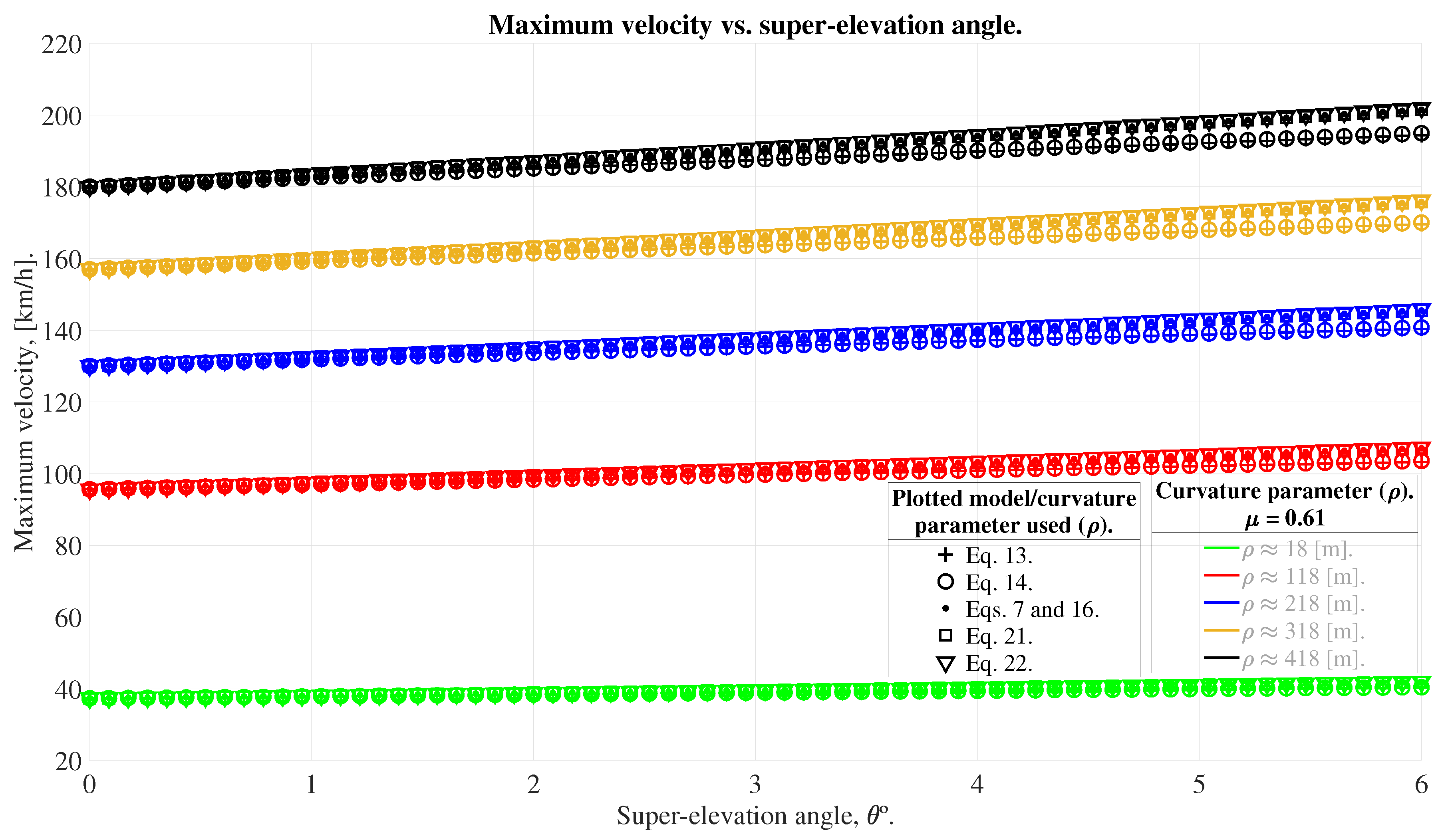
4. Results Comparative Presentation and Discussion

In this section, results from the models developed in the preceding one are presented and compared. The objective was to solve for the maximum highway speed without slippage between vehicle and pavement, which constitutes a reasonable estimate of a motor road’s maximum safe operational speed. They reflect the broad versatility of classical dynamics applied to the problem.

The analytical results obtained can be condensed in the following table (

Table 1. Summary of results for safe highway operating speeds v for different models. Geometrophysical parameters used are motion curvature radius (R) or intrinsic radial (r) coordinate to the specific model, the friction coefficient between vehicle and pavement ($\mu$), and highway super-elevation ($\theta$). g is the gravitational acceleration’s magnitude considered constant for the analysis.

Geometric Model	Curvature Parameter	Maximum Speed
“n & t”/unrotated cylindrical-polar system (Equation (7)/Equation (16))	R	$v=\sqrt{\frac{gR\left(sin\theta +\mu cos\theta \right)}{cos\theta -\mu sin\theta }}$
Rotated cylindrical-polar system (Equation (13))	r	$v=\sqrt{gr(sin\theta +\mu cos\theta )}$
Rotated cylindrical-polar system (Equation (14))	R	$v=\sqrt{gR(\mu +tan\theta )}$
Spherical system (Equation (21))	R	$v=\sqrt{\frac{grsec\theta (\mu +tan\theta )}{1-\mu tan\theta }}$
Spherical system (Equation (22))	r	$v=\sqrt{\frac{gR\left(\mu +tan\theta \right)}{1-\mu tan\theta }}$

).

The visible points of interest are the following:

(1) Mathematically (i.e., symbolically) comparing equations Equations (2), (13), and (14), it is noticeable that a worldwide used model in regulations is analytically similar/equivalent to the models represented by Equations (13) and (14), particularly the latter. That is, the model expressed in Equation (2) is a slight re-parametrization of Equation (13), mainly in order to consider friction as a demand parameter. Therefore, one of the most used models regarding regulations on highway speeds is a 2D native one applied to a 3D organic situation, as explained in the previous section.

(2) As expected, the normal–tangential coordinate motion description (Figure 1, Equation (7)) and the unrotated cylindrical-polar system coordinate motion description (Figure 5, Equation (16)) models are completely analytically equivalent. A non-analytical difference, but conceptually substantial, is related to the nature of the motion curvature parameter used. In the former, the circular trajectory curvature radius (R) is in a plane parallel to that used for super-elevation measurement. Notice that this definition is only possible by adding a new coordinate normal to the “n & t” original set, ad-hoc to the problem; that is, an ad-hoc renderization of a 2D situation into a 3D one is required. Now, in the latter, the coordinate “added” is one of the natural coordinates of the model, the radial one (r). The plane of motion considered is also parallel to that used for super-elevation measurement.

(3) In Equation (12), the acceleration does not have components in addition to the radial one because the cylindrical-polar coordinate system as a whole rotated with respect to the horizontal plane is considered, an angle amounting to the highway super-elevation $\theta$. In such a system, the motion studied does not take place on the horizontal Cartesian plane $\widehat{x}-\widehat{y}-\widehat{z}$ but in the rotated plane $\widehat{r}-\widehat{\varphi }-\widehat{z}$ described by the cylindrical-polar coordinate system, as shown in Figure 4. The radial direction $\widehat{r}$ is then perpendicular to the studied motion’s tangential direction. In other words, in the instant represented in Figure 4, $\widehat{\varphi }$ enters the scene. Since $\widehat{\varphi }$ becomes the motion’s tangential direction in this particular model, the calculation for an assumed constant maximum velocity without any slippage requires three things. First, radial velocity ($v_r\widehat{r}$) and acceleration ($a_r\widehat{r}$) components must be null, implying that $\dot{r}=\ddot{r}=0$ in Equation (9). Second, polar velocity ($v_{\varphi }\widehat{\varphi }$) must remain constant (that is, $\dot{\varphi }=constant$, $\ddot{\varphi }=0$ in Equation (9)). Third, there must be no velocity and acceleration in the $\widehat{z}$ direction ($\dot{z}=\ddot{z}=0$). Consequently, instantaneously solving Equation (12) leads us to Equations (13) with r and (14) with R, which differ from Equations (7), (16), (21), and (22).

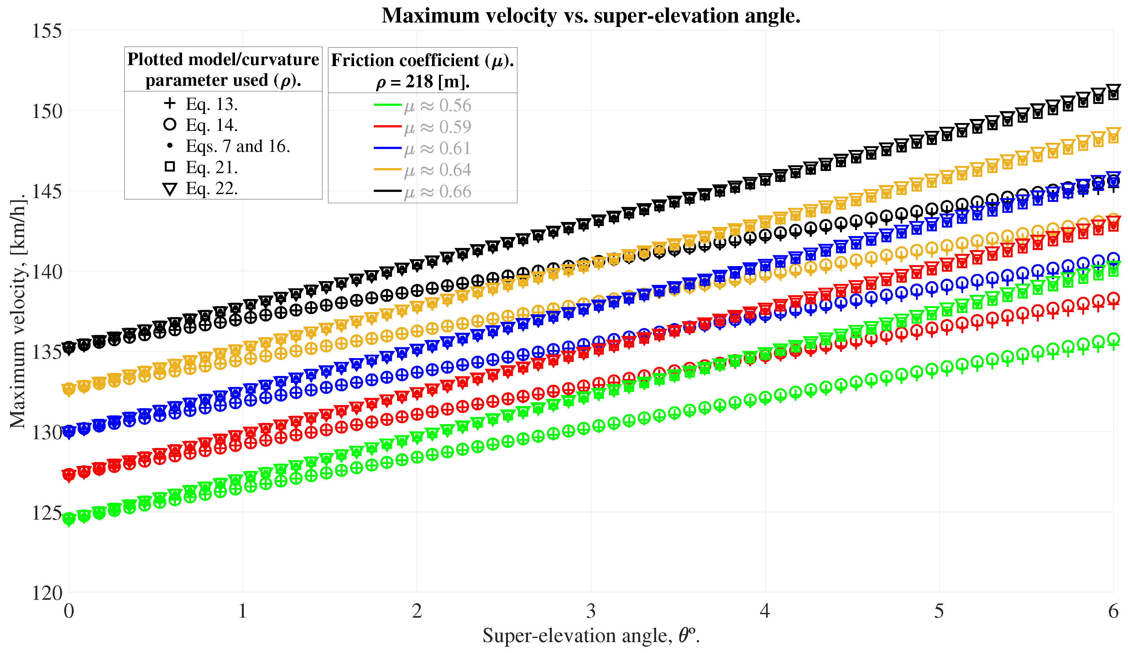
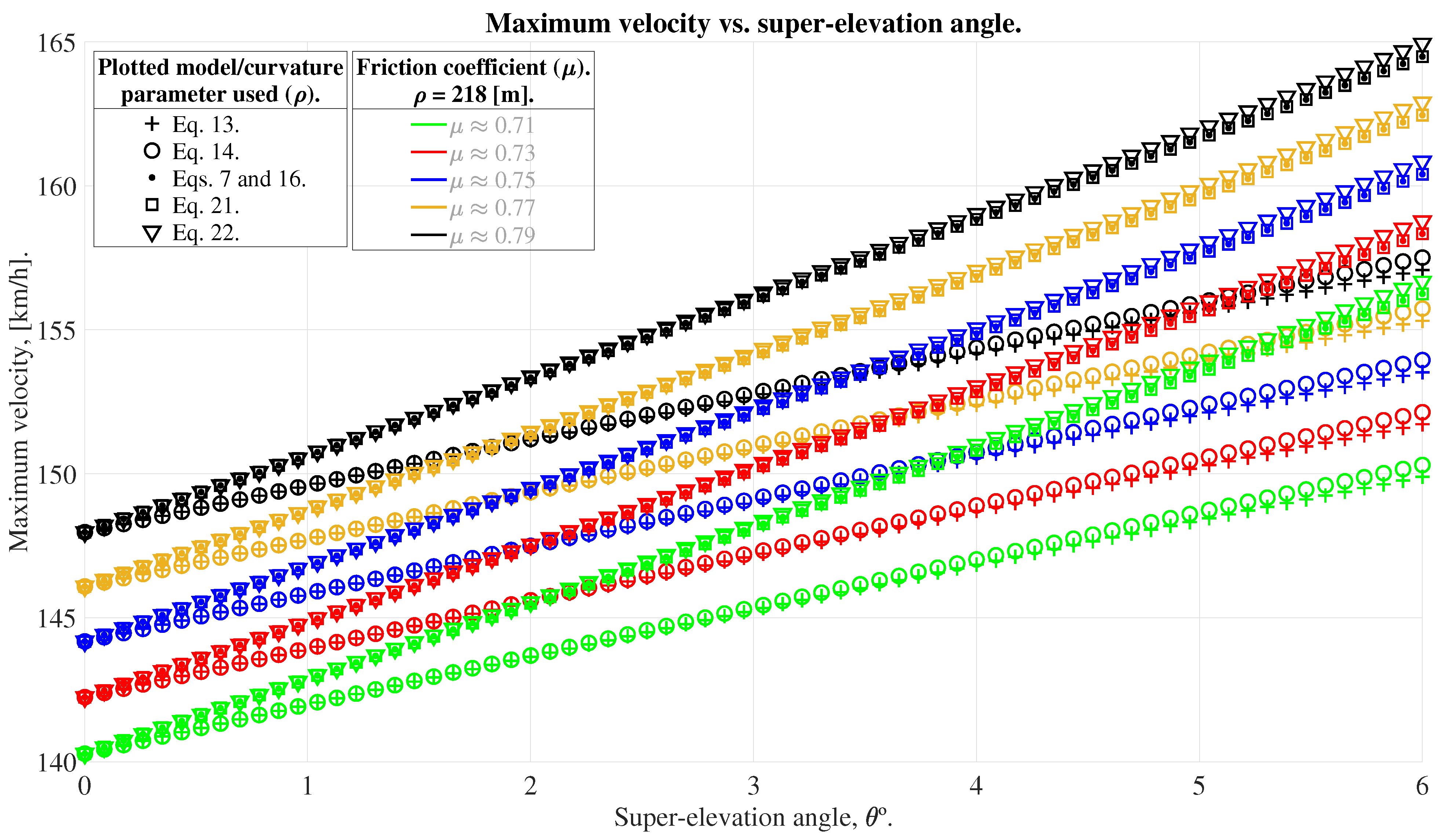
5. Parametric Sweep: Visualization and Analysis

In order to compare models among them, an assessment of the parameters involved must be conducted first. There are four of them: r, R, $\theta$, and $\mu$. Regarding the last one, the friction coefficient between pavement and vehicle ($\mu$) is an experimentally obtained parameter. Naturally, it has a physical nature, though not much of a geometrophysical one in the sense implied here. The remaining parameters are fully geometrophysical since they arise from analyzing and applying different conceptual/geometrophysical models over the problem of interest discussed previously. Therefore, the parametric set up is shown in

Table 2. Mexico’s governmental sanctioned highway design parameters. Extracted from [18].

Parameter	Parametric Range	Parameter Mean
Curvature radius	$19.1\le R\le 416.7\left[m\right]$	∼$218\left[m\right]$
Super-elevation	$0^{\circ }\le \theta \le 5.{71}^{\circ }$	∼$3^{\circ }$
Maximum speed	$30\le v\le 110[km/h]$	∼$70[km/h]$

, according to Mexico’s governmental agency in charge of highway design regulations [18] and experimental procedures in

Table 3. Experimentally obtained friction coefficients under different conditions between tire rubber and pavement. Contact/interface area at temperatures including −10 [°C] $\le T\le 0$ [°C]. Extracted from [27].

Pavement Particular Conditions	Parametric Range	Parameter Mean	Mean Particle Diameter
Iced, no sand	$0.10\le {\mu }_s\le 0.23$	∼$0.1650$	Not applicable.
Dry, sandy	$0.56\le {\mu }_s\le 0.66$	∼$0.61$	∼$176\left[\mu m\right]$
Dry, sandy	$0.71\le {\mu }_s\le 0.79$	∼$0.75$	∼${10}^3\left[\mu m\right]$

, fully described in [27].

Figure 7, Figure 8, Figure 9, Figure 10, Figure 11 and Figure 12 show the graphical results of the parametric analysis proposed. Before briefly discussing them, analytical calculations were developed on default MATLAB R2022b computational machine precision, retaining three significant digits due to friction coefficient experimental values (significant figures) in [27].

On the other hand, as expressed in the figure captions, the calculations for percentage relative errors took as reference the rotated cylindrical/radial coordinate model in Equations (13) and (14) due to its analytical/conceptual proximity to the model in Equation (2), as explained in previous sections: the model in Equation (2) is a reasonable numerical approximation of the model in Equation (1). Concurrently, the models in Equations (13) and (14) are equivalent among them (when switching the curvature parameter considered, i.e., $r\to R$) and also a straight forward reparametrization of the model in Equation (2).

Figure 7. Maximum velocity vs. super-elevation angle. $18\lesssim \rho \lesssim 418\left[m\right]$, $\mu =0.61$. $\rho$ is the curvature parameter used, whether r or R. Pavement conditions: dry, sandy. Sand particle mean diameter ∼$176\left[\mu m\right]$. In this figure, the percentage relative errors between models, having as a reference the rotated cylindrical/curvature radius (that is presented in Equation (14)), vary between $0\le \%E\le 3.65$.

Figure 7. Maximum velocity vs. super-elevation angle. $18\lesssim \rho \lesssim 418\left[m\right]$, $\mu =0.61$. $\rho$ is the curvature parameter used, whether r or R. Pavement conditions: dry, sandy. Sand particle mean diameter ∼$176\left[\mu m\right]$. In this figure, the percentage relative errors between models, having as a reference the rotated cylindrical/curvature radius (that is presented in Equation (14)), vary between $0\le \%E\le 3.65$.

Figure 8. Maximum velocity vs. super-elevation angle. $0.56\lesssim \mu \lesssim 0.66$, $\rho =218\left[m\right]$. $\rho$ is the curvature parameter used, whether r or R. Pavement conditions: dry, sandy. Sand particle mean diameter ∼$176\left[\mu m\right]$. In this figure, the percentage relative errors between models, having as a reference the rotated cylindrical/curvature radius (that is presented in Equation (14)), vary between $0\le \%E\le 3.94$.

Figure 8. Maximum velocity vs. super-elevation angle. $0.56\lesssim \mu \lesssim 0.66$, $\rho =218\left[m\right]$. $\rho$ is the curvature parameter used, whether r or R. Pavement conditions: dry, sandy. Sand particle mean diameter ∼$176\left[\mu m\right]$. In this figure, the percentage relative errors between models, having as a reference the rotated cylindrical/curvature radius (that is presented in Equation (14)), vary between $0\le \%E\le 3.94$.

Figure 9. Maximum velocity vs. super-elevation angle. $18\lesssim \rho \lesssim 418\left[m\right]$, $\mu =0.75$. $\rho$ is the curvature parameter used, whether r or R. Pavement conditions: dry, sandy. Sand particles mean diameter ∼${10}^3\left[\mu m\right]$. In this figure, the percentage relative errors between models, having as a reference the rotated cylindrical/curvature radius one (that presented in Equation (14)), vary between $0\le \%E\le 4.47$.

Figure 9. Maximum velocity vs. super-elevation angle. $18\lesssim \rho \lesssim 418\left[m\right]$, $\mu =0.75$. $\rho$ is the curvature parameter used, whether r or R. Pavement conditions: dry, sandy. Sand particles mean diameter ∼${10}^3\left[\mu m\right]$. In this figure, the percentage relative errors between models, having as a reference the rotated cylindrical/curvature radius one (that presented in Equation (14)), vary between $0\le \%E\le 4.47$.

Figure 10. Maximum velocity vs. super-elevation angle. $0.71\lesssim \mu \lesssim 0.79$, $\rho =218\left[m\right]$. $\rho$ is the curvature parameter used, whether r or R. Pavement conditions: dry, sandy. Sand particle mean diameter ∼${10}^3\left[\mu m\right]$. In this figure, the percentage relative errors between models, having as a reference the rotated cylindrical/curvature radius (that is presented in Equation (14)), vary between $0\le \%E\le 4.71$.

Figure 10. Maximum velocity vs. super-elevation angle. $0.71\lesssim \mu \lesssim 0.79$, $\rho =218\left[m\right]$. $\rho$ is the curvature parameter used, whether r or R. Pavement conditions: dry, sandy. Sand particle mean diameter ∼${10}^3\left[\mu m\right]$. In this figure, the percentage relative errors between models, having as a reference the rotated cylindrical/curvature radius (that is presented in Equation (14)), vary between $0\le \%E\le 4.71$.

Figure 11. Maximum velocity vs. super-elevation angle. $18\lesssim \rho \lesssim 418\left[m\right]$, $\mu =0.165$. $\rho$ is the curvature parameter used, whether r or R. Pavement conditions: icy, no sand. In this figure, the percentage relative errors between models, having as a reference the rotated cylindrical/curvature radius (that is presented in Equation (14)), vary between $0\le \%E\le 1.15$.

Figure 11. Maximum velocity vs. super-elevation angle. $18\lesssim \rho \lesssim 418\left[m\right]$, $\mu =0.165$. $\rho$ is the curvature parameter used, whether r or R. Pavement conditions: icy, no sand. In this figure, the percentage relative errors between models, having as a reference the rotated cylindrical/curvature radius (that is presented in Equation (14)), vary between $0\le \%E\le 1.15$.

Figure 12. Maximum velocity vs. super-elevation angle. $0.1\lesssim \mu =\lesssim 0.23$, $\rho =218\left[m\right]$. $\rho$ is the curvature parameter used, whether r or R. Pavement conditions: icy, no sand. In this figure, the percentage relative errors between models, having as a reference the rotated cylindrical/curvature radius (that is presented in Equation (14)), vary between $0\le \%E\le 1.50$.

Figure 12. Maximum velocity vs. super-elevation angle. $0.1\lesssim \mu =\lesssim 0.23$, $\rho =218\left[m\right]$. $\rho$ is the curvature parameter used, whether r or R. Pavement conditions: icy, no sand. In this figure, the percentage relative errors between models, having as a reference the rotated cylindrical/curvature radius (that is presented in Equation (14)), vary between $0\le \%E\le 1.50$.

The first thing to notice is that there are indeed differences between models over maximum speeds before tires/pavement slippage. That is interesting since this involves a model (Equation (2)) that has been used for many years and constitutes the basis for numerous national regulatory systems, scantly discussed in terms of fundamentals such as the ones brought up here. It is not claimed here that the model has been a liability per-se. However, this finding could represent an opportunity to work on the lack of discussion of principles about the geometrophysical parameters involved in the general problem, such as the concepts of curvature radius and (highway) super-elevation and, furthermore, about concepts such as vehicle trajectory in these kinds of applications.

Another interesting feature of the results is that the smaller differences between models are found in the most slippery conditions, Cf. Figure 9, Figure 10, Figure 11 and Figure 12. That is perhaps counter-intuitive since an icy pavement surface conveys edgy model conditioning. On the other hand, if icy pavement implies the smaller-in-value non-geometrophysical parameter under consideration (Cf. Table 3), the results appear reasonable. Indeed, a comparison of Figure 8, Figure 9 and Figure 10 shows that the sequence of model differences continues to augment with increasing friction coefficient values (${\overline{\mu }}_s=0.61$, $\%E_{Max}=3.94$, and ${\overline{\mu }}_s=0.75$, $\%E_{Max}=4.71,$ respectively). Please Cf. Table 3 again.

As explained in Section 3.2, it has been established that models leading to Equations (13) and (14) are mathematically equivalent to the model expressed in Equation (2), Cf. [25]. This equivalence allows for the utilization of the former (Equation (14)) as a reference for comparison. This finding is particularly interesting since, to the best of our knowledge, this specific topic has not been addressed in the existing literature. Of course, the broader subject of developing and applying point mass models regarding the main problem reviewed by this paper is known, as well as the recognition that the model represented by Equation (2) is derived from practical approximation considerations applied to the model proposed by Equation (1), as explained in earlier sections. However, a quantitative analysis of this relationship and its derived consequences, as proposed in this study, has not been previously conducted.

Other analytical features of interest displayed in the figures are quite reasonable. Among them, the fact that the two 2D models by conception (Equations (13) and (14)) are lumped together against the others in all figures. Furthermore, the differences between models in Equations (13) and (14) are of $\%E_{Max}\sim 0.27$, manifesting that solely considering another curvature parameter in nature generates differences (r or R). That lumping could be explained precisely for the former reason. Those two models are 2D approximations of a 3D situation; therefore, in principle, they are conceptually more inaccurate than their counterparts in Equations (16), (21), (22). Another one, in addition to reasonable, and also to be expected, is the analytical equivalence of models in Equations (7), (16), (21); which accounts for the fact that a given geometrophysical situation can be conceptualized in several equivalent ways. For example, if one multiplies the left-hand side of Equations (7) or (16) with $\frac{1/cos\theta }{1/cos\theta }$, Equation (22) is obtained. Notice that this is made possible because of the loose and formally/conceptually problematic notion of a radius of curvature parameter (R), as discussed in previous sections (Cf. Table 1). In summary, modeling a real physical situation using different geometrophysical sets produces equivalent results, provided the models are mutually reducible among them. If that is not the case, differences arise, such as in the case of models in Equations (22) and (14).

Finally, for México’s particular case, the main finding of this work is that the model used as the regulatory basis for calculating the safe speeds of highways has a percentage of relative error differences with respect to the others under consideration. Moreover, the differences found in principle favor safe highway operation, since the IRCM-inspired model (Equations (2) and (14)) consistently predicts lower speeds than the others (Cf. Figure 7, Figure 8, Figure 9, Figure 10, Figure 11 and Figure 12). If that is experimentally verified, which is outside the proposed scope of this work, the relevant potential consequences of the present discussion would be primarily related to, for example, the economic logistics of highway design, construction, and operation, important subjects within this paper’s overall context but also outside its proposed scope.

6. Observations/Conclusions

This study consolidates the results regarding the impact of geometric and physical modeling considerations on road and highway design related to México’s case. It was observed that different parametrizations of the same scenario can lead to diverse outcomes not previously foreseen/documented in Mexico’s regulations or reported elsewhere. Particularly, there are significant differences in the maximum safe operating velocities when considering variation in concepts such as plane of motion and curvature parameter, i.e., R (radius of curvature) and r (model’s natural radial coordinate), which necessitate further investigation.

Therefore, this study’s findings call for experimental research in order to fully establish and explore the potential implications of these differences on highway design, emphasizing that relative variations between models peak at approximately $\%E_{Max}\sim 5$, a critical parametric value in specific foreseeable situations. For example, in scenarios involving extreme conditions such as vehicle motion on race tracks, competitions, or park attractions, these effects are likely to be more pronounced, pointing to a need for additional focused research. Particularly, both end possibilities, that is, whether the reference model for México’s highway regulations is underestimating (which seems to be the actual case according to the discussed findings) or overestimating maximum safe operational speeds, are conducive to interesting lines of further exploration.

Finally, while the study presented here primarily adopted a conceptual and analytical approach, it also highlighted the necessity for a comprehensive experimental framework to align the involved conceptual and geometrophysical aspects with practical applications. This dual approach underscores the complexity and prospective relevance of these preliminary findings to both the theoretical and practical aspects of highway engineering. Succinctly put, beyond the overall approach described in this work, which is conceptual in inception and analytical in discussion of results, a comprehensive experimental approach to the problem complementary to the one presented is required to compare its conceptual/geometrophysical aspects to practical ones.

References

1. Ma, Y.; Mi, J.; Yang, X.; Sun, Z.; Liu, C. Prediction model and sensitivity analysis of ultimate drift ratio for rectangular reinforced concrete columns failed in flexural-shear based on BP-Garson algorithm. Structures 2024, 60, 105808. [Google Scholar] [CrossRef]
2. Liu, C.; Zhao, B.; Yang, J.; Yi, Q.; Yao, Z.; Wu, J. Effects of brace-to-chord angle on capacity of multi-planar CHS X-joints under out-of-plane bending moments. Eng. Struct. 2020, 211, 110434. [Google Scholar] [CrossRef]
3. Montella, A.; Galante, F.; Mauriello, F.; Aria, M. Continuous speed profiles to investigate drivers’ behavior on two-lane rural highways. Transp. Res. Rec. 2015, 2521, 3–11. [Google Scholar] [CrossRef]
4. Choi, J.; Tay, R.; Kim, S. Effects of changing highway design speed. J. Adv. Transp. 2013, 47, 239–246. [Google Scholar] [CrossRef]
5. Shaon, M.R.R.; Qin, X.; Chen, Z.; Zhang, J. Exploration of contributing factors related to driver errors on highway segments. Transp. Res. Rec. 2018, 2672, 22–34. [Google Scholar] [CrossRef]
6. Fitzpatrick, K.; Zimmerman, K. Potential updates to 2004 green book’s acceleration lengths for entrance terminals. Transp. Res. Rec. 2007, 2023, 130–139. [Google Scholar] [CrossRef]
7. Figueroa-Medina, A.; Tarko, A. Reconciling speed limits with design speeds. Jt. Transp. Res. Program 2004, FHWA/IN/JTRP-2004/26. [Google Scholar]
8. Fu, M. Research on Superelevation Design in Highway Route Design. J. World Archit. 2021, 5. [Google Scholar] [CrossRef]
9. Abdulhafedh, A. Design of superelevation of highway curves: An overview and distribution methods. J. City Dev. 2019, 1, 35–40. [Google Scholar]
10. Craus, J.; Livneh, M. Superelevation and curvature of horizontal curves. Transp. Res. Rec. 1978, 685, 7–13. [Google Scholar]
11. Himes, S.; Porter, R.; Hamilton, I.; Eric, D. Safety evaluation of geometric design criteria: Horizontal curve radius and side friction demand on rural, two-lane highways. Transp. Res. Rec. 2019, 2673, 516–525. [Google Scholar] [CrossRef]
12. Jiang, F.; Sun, X.; Li, H.; Huang, J.; Li, D. Optimization Analysis of Minimum Flat Curve Radius of High Speed Maglev Line with Design Speed of 500 km/h. In Proceedings of the IOP Conference Series: Materials Science and Engineering, Sabah, Malaysia, 9–11 August 2019; Volume 637, pp. 012008–012015. [Google Scholar]
13. Nazmul, H. Maximum allowable speed on curve. In Proceedings of the ASME/IEEE Joint Rail Conference, Pueblo, CO, USA, 16–18 March 2011; Volume 54594, pp. 1–9. [Google Scholar]
14. Richl, L.; Sayed, T. Effect of speed prediction models and perceived radius on design consistency. Can. J. Civ. Eng. 2005, 32, 388–399. [Google Scholar] [CrossRef]
15. Schurr, K.; McCoy, P.; Pesti, G.; Huff, R. Relationship of design, operating, and posted speeds on horizontal curves of rural two-lane highways in Nebraska. Transp. Res. Rec. 2002, 1796, 60–71. [Google Scholar] [CrossRef]
16. Miaou, S.P.; Lum, H. Modeling vehicle accidents and highway geometric design relationships. Accid. Anal. Prev. 1993, 25, 689–709. [Google Scholar] [CrossRef] [PubMed]
17. Vayalamkuzhi, P.; Amirthalingam, V. Influence of geometric design characteristics on safety under heterogeneous traffic flow. J. Traffic Transp. Eng. 2016, 3, 559–570. [Google Scholar] [CrossRef]
18. Ruiz, G.; Callejo, O.; Verdugo, J. Manual de proyecto geométrico de carreteras 2018. 2018. Available online: http://sct.gob.mx/normatecaNew/manual-de-proyecto-geometrico-de-carreteras/ (accessed on 6 May 2024).
19. Albattah, M. Optimum highway design and site location using spatial geoinformatics engineering. J. Remote Sens. GIS 2016, 5, 10. [Google Scholar]
20. Boas, P.R.V.; Rodrigues, F.A.; Costa, L.d.F. Modeling worldwide highway networks. Phys. Lett. A 2009, 374, 22–27. [Google Scholar] [CrossRef]
21. Biancardo, S.A.; Capano, A.; de Oliveira, S.G.; Tibaut, A. Integration of BIM and procedural modeling tools for road design. Infrastructures 2020, 5, 37. [Google Scholar] [CrossRef]
22. Wang, Y.; Wang, W.; Liu, J.; Chen, T.; Wang, S.; Yu, B.; Qin, X. Framework for geometric information extraction and digital modeling from LiDAR data of road scenarios. Remote Sens. 2023, 15, 576. [Google Scholar] [CrossRef]
23. Qi, H.; Cong, B.; Liu, R.; Li, X.; Yan, Z.; Li, Q.; Li, M. Research on the 3D fine modeling method of In-service road. Adv. Civ. Eng. 2023, 2023, 7336379. [Google Scholar] [CrossRef]
24. Wei, Y.; Zhang, Z.; Huang, X.; Lin, Y.; Liu, W. 3D highway curve reconstruction from mobile laser scanning point clouds through deep reinforcement learning. Int. Arch. Photogramm. Remote Sens. Spat. Inf. Sci. 2023, 48, 55–61. [Google Scholar] [CrossRef]
25. AASHTO. A Policy on Geometric Design of Highways and Streets; AASHTO (American Association of State Highway and Transportation Officials): Washington, DC, USA, 2011. [Google Scholar]
26. Echaveguren, T.; Bustos, M.; De Solminihac, H. Assessment of horizontal curves of an existing road using reliability concepts. Can. J. Civ. Eng. 2005, 32, 1030–1038. [Google Scholar] [CrossRef]
27. Hurtado, A. Estudio del Coeficiente de Fricción en Asfalto con Presencia de Hielo y Arena Empleando el péndulo Deslizante. Master’s Thesis, Instituto Politécnico Nacional, Ciudad de México, México, 2017. [Google Scholar]
Figure 3. General layout of the problem and the geometrophysical scheme applied to account for it. In this figure, R is the parameter of the curvature considered (in this case, a radius of curvature), and v is the vehicle’s velocity.
Applsci 14 04064 g003
Figure 4. Dynamic situation description in terms of cylindrical-polar coordinates: “normal”, “tangential”, and z coordinates; that is, ( r ; ϕ ; z ). Plane of motion considered rotated with respect to horizontal plane. In this figure, N , F , and W are the forces acting on the vehicle: normal, friction, and weight, respectively. The angle θ is the highway’s considered super-elevation; R is the radius of curvature (curvature parameter considered). r ^ , ϕ ^ , z ^ are the 3D cylindrical-polar coordinate system unit vectors.
Applsci 14 04064 g004
Figure 5. Dynamic situation description in terms of cylindrical-polar coordinates: “normal”, “tangential”, and z coordinates; that is, ( r ; ϕ ; z ). Plane of motion considered unrotated (i.e., parallel) with respect to the horizontal plane. In this figure, N , F , and W are the forces acting on the vehicle: normal, friction, and weight, respectively. The angle θ is the highway’s considered super-elevation. r ^ , ϕ ^ , and z ^ are the 3D cylindrical-polar coordinate system unit vectors.
Applsci 14 04064 g005
Figure 6. Dynamic situation description in terms of spherical coordinates: “radial”, “azimuthal”, and “zenithal” coordinates; that is, ( r ; ϕ ; ψ ). Plane of motion considered unrotated with respect to the horizontal plane. In this figure, N , F , and W are the forces acting on the vehicle: normal, friction, and weight, respectively. The angle θ is the highway’s considered super-elevation; R is the radius of curvature (curvature parameter considered). r ^ , ϕ ^ , and ψ ^ are the 3D spherical coordinate system unit vectors.
Applsci 14 04064 g006