
A Spacecraft Onboard Autonomous Task Scheduling Method Based on Hierarchical Task Network-Timeline

1
Key Laboratory of Electronics and Information Technology for Space System, National Space Science Center, Chinese Academy of Sciences, Beijing 100190, China
2
University of Chinese Academy of Sciences, Beijing 100049, China
*
Author to whom correspondence should be addressed.
Aerospace 2024, 11(5), 350; https://doi.org/10.3390/aerospace11050350
Submission received: 25 March 2024
/
Revised: 24 April 2024
/
Accepted: 25 April 2024
/
Published: 27 April 2024
(This article belongs to the Section Astronautics & Space Science)
Abstract
:To address the inherent challenges of deep space exploration, such as communication delays and the unpredictability of spacecraft environments, this study focuses on enhancing spacecraft adaptability and autonomy, which are essential for Autonomous Space Scientific Exploration. A pivotal aspect of this endeavor is the advancement of spacecraft task scheduling, which is integral to increasing spacecraft autonomy. Current research in this domain predominantly revolves around mission timing planning and is primarily executed from ground stations. However, these plans often lack the granularity required for direct implementation by spacecraft. In response, our study proposes an innovative approach to augment spacecraft autonomy, introducing a method that articulately describes mission objectives and resource information. We designed a novel hierarchical task network-timeline (HTN-T) algorithm, an amalgamation of the HTN scheduling method and the distinctive elements of existing research. This algorithm addresses time constraints through horizontal and vertical expansions, building upon the resolution of logical constraints found in conventional planning methods. Furthermore, it introduces a priority-based strategy for resolving resource conflicts in spacecraft tasks. This algorithm is substantiated through validation, including proof-of-principle demonstrations and assessments within a Space–ground Collaborative Management and Control System encompassing both ground and spacecraft operations. The findings indicate that our proposed algorithm achieves high rates of scheduling success and operational efficiency within a feasible timeframe, thus effectively navigating the complexities of autonomous spacecraft task scheduling.
1. Introduction
The advancement of deep space exploration has posed significant challenges to traditional spacecraft operation modes. On the one hand, longer terrestrial and satellite communication distances cause long communication delays, which are more unfavorable for real-time control. On the other hand, the environment of deep space is uncertain, which makes it more difficult for spacecrafts to make convincing decisions in this environment. It is foreseeable that, over time, the future of deep space exploration will transform from “target-specific Scientific Space Exploration” to “Autonomous Scientific Space Exploration”. Such autonomy requires spacecrafts to achieve “self-adaptation” to the environment, scientific goals, and their state.
Autonomous Space Scientific Exploration (ASSE) is a new concept that has become popular recently. It is a process wherein spacecrafts undertake scientific exploration missions, whether known or unknown. In this process, the spacecraft can be independent of the ground and based on some limited onboard capabilities, resources, and knowledge, make its own decisions. The core of this “self-adaptation” is using modern control technology to determine the spacecraft’s operation strategy based on telemetry data and the environment, independently of ground operators. Simultaneously, spacecrafts must maintain high precision, exceptional stability, robust adaptability, unparalleled reliability, and an extended operational life. The capabilities of “Autonomous Scientific Space Exploration” include the autonomous management of resource information, mission decision making, planning and scheduling, self-discovery of task objectives, self-monitoring of on-orbit operation status, autonomous repair, etc. The research in task decision making, planning, and scheduling will be significant because of its close relationship to realizing the spacecraft’s scientific objectives.
Building on the previous analysis, there is a pressing need to develop an onboard autonomous task scheduling method specifically tailored for spacecraft payloads, predicated on the concept of system-level autonomy. System-level autonomy means the autonomous capability of a spacecraft is not confined to specific payloads or functions but rather involves the integrated coordination and execution of various capabilities. It leverages the current environment and relevant engineering parameters to fulfill the spacecraft’s mission objectives. System-level autonomy requires the spacecraft to independently execute the appropriate command sequences according to the external environment after knowing the objectives, i.e., the spacecraft’s traditional “behavior-driven” operational mode to a more sophisticated “objective-driven” paradigm.
The motivation of this research is to work on solving the time and resource description problem of hierarchical task networks onboard, designing corresponding algorithms to maximize the execution efficiency of tasks and the optimal allocation of resource conflicts, and realizing onboard autonomous task scheduling for spacecraft payloads. This will enable the spacecraft and its payload to autonomously complete the operations according to the environment and task objectives.
Based on this, the main contributions of this paper are as follows:
- To construct the spacecraft’s autonomous capability, we designed a method describing the objectives.
- Utilizing the hierarchical task network (HTN) method, we designed a hierarchical task network-timeline (HTN-T) method based on the spacecraft intelligence architecture, which addresses both the logical and time constraints in spacecraft task scheduling through horizontal and vertical extensions.
- We also crafted a priority-based conflict resolution strategy for managing spacecraft task resources, aiming at their optimal allocation.
- Through simulation testing, we verified the effectiveness of the spacecraft’s autonomous task-scheduling algorithm.
2. Related Work
With the popularization of autonomous systems and the increased demand for spacecraft autonomy, research on spacecraft task planning and scheduling is rising, and both are of great significance. Initially, this planning was accomplished using methods such as first-order logic [1] and scenario algorithms [2]. Subsequently, the Stanford Research Institute Problem Solver (STRIPS) planning description was proposed by Nillson [3], marking a pivotal advancement. Influenced by STRIPS, McDermott et al. introduced the Planning Domain Definition Language (PDDL) in 1998 [4], further enriching the field. The Automated Scheduling and Planning ENvironment (ASPEN) system [5] of the National Aeronautics and Space Administration (NASA) represented another leap forward. It constructs a task description model based on iterative restoration. This system has been deployed on satellites, including EO-1, and other satellites implemented software for imaging scheduling systems based on ASPEN [6]. Building on ASPEN’s foundation, Chien et al. partially integrated it with the greedy algorithm, enhancing the description methodology [7]. The French Space Agency’s Pleiades satellite employs the Autonomy Generic Architecture—Tests and Application (AGATA) for task planning, which can be carried out on board with a timeline-based constraint network approach. [8] NASA has developed the Extensible Uniform Remote Operational Planning Architecture (EUROPA) system and the Mixed-Initiative Activity Plan Generator (MAPGEN), which were applied to the Mars Exploration Missions Courage and Opportunity [9]. Similarly, the Spike system, built on CSP [10], has been utilized for the surface roving missions of the Mars rovers Courage and Opportunity, as well as servicing the Hubble Telescope. This evolution underscores the dynamic progress of onboard planning and its critical role in advancing ASSE.
Recent studies on task scheduling and integrating artificial intelligence and intelligent algorithms have seen a notable increase. These studies leverage a variety of methods, including heuristic algorithms, artificial neural networks (ANNs), deep reinforcement learning (DRL), semiotics-based AI, and so on. For instance, Shi Janshun et al. developed a deep deterministic policy gradient (DDPG) algorithm for space station mission replanning based on DRL. This method enables finding near-optimal solutions through the algorithm’s continuous evolution, overcoming the constraints of preset conflict resolution strategies [11]. Liu Yang et al. also devised a priority-based scheduling algorithm for load-level tasks, accounting for both task-resource limitations and spacecraft conditions, including external conditions, power supply, and storage [12]. Yao Min et al. created a mission flow autonomous planning system, tailored to spacecraft payload and task requirements [13]. NASA designed the Framework for Robust Execution and Scheduling of Commands Onboard (FRESCO), which achieves the system-level autonomy of the spacecraft, and the Arcsecond Space Telescope Enabling Research In Astrophysics CubeSat workstation [14]. Furthermore, Jun Liang et al. designed a precedence-rule-based heuristic for satellite onboard activity planning. It is used in the description of onboard activity domain knowledge and aimed at reducing the completion time for onboard activities [15].
Synthesizing the above research status of spacecraft task planning and scheduling, the following features can be summarized:
- Most of the task planning and scheduling methods are overwhelmingly focused on sequencing planning. For example, temporal sequencing planning for the shooting locations of imaging satellites, path planning for the flight trajectories of spacecrafts, and so on. The planning results of these methods are more granular; they cannot be directly executed as spacecraft commands without further processing. Therefore, this approach cannot be directly applied to the problem of autonomous mission planning onboard spacecrafts.
- Moreover, the existing approach necessitates uploading the scheduling results to the spacecraft through the communication link instead of executing the planning process directly onboard. These methods are still challenging when it comes to solving the spacecraft communication delay problem in deep space exploration.
- In addition, many spacecraft mission planning and scheduling studies are isolated studies that are not integrated with the spacecraft software architecture. In the specialized field of spacecraft intelligence architecture, Lyu L. et al. have put forward an innovative spacecraft intelligence software architecture [16]. Autonomous mission scheduling methods for spacecrafts need to be adequately supported by similar architectures in order to realize their potential in practical scientific exploration.
The HTN approach is a common solution for task objective-based scheduling. This method is an artificial intelligence technique for solving domain planning problems [17]. Its advantages, including sufficient interpretability, modularity, maintainability, and adaptability, establish it as an effective tool for solving complex task planning and decision-making problems. The most significant feature of the method is its domain modeling capabilities—the ability to complete modeling and solving in alignment with real-world scenarios.
The HTN has been successfully applied in various objective-based aerospace fields, underscoring its effectiveness in sophisticated planning tasks [18]. However, existing HTN descriptions tend to focus primarily on the sequential logical relationship between tasks; the resource conflict and time description of tasks are relatively lacking. Meanwhile, the challenge of implementing common hierarchical task networks onboard still belongs to the research gap. There is an urgent requirement to combine the existing solutions to forge a task description methodology on the spacecraft and complete the deployment of the algorithm.
3. Objective-Driven and Task Objective Command
The remote operation of spacecrafts includes sending remote-control commands to the ground and receiving telemetry data. To carry out the standardized design of remote-control and telemetry data, the Consultative Committee for Space Data Systems (CCSDS) has carried out a standard encapsulation of remote-control commands in space packages and designed the Telemetric and Command Exchange described by XML [19], which defines the data format for spacecraft remote control and telemetry [20]. The European Space Agency (ESA) then launched a package standard compatible with it [21]. It solves the application problems of space packages not given by the CCSDS and provides an effective way to generalize remote-control commands. This paper’s data-injection format is based on the format specified in the space package protocol CCSDS 133.0-B-1 [22], which is shown in Table 1.
The Space Packet consists of a Packet Header, Packet Secondary Header, and User Data Field. Within the User Data Field are multiple Command Packets, each filled with specific information in its Packet Data Field. This structure is commonly used for data injection and has been applied in practical engineering projects.
Defining “action” as the basic unit that prompts spacecrafts to alter their state and complete tasks is known as “action-driven”. Autonomous Scientific Space Exploration requires using task objectives as the foundational unit to enable the spacecraft’s autonomous decision making. It needs to use targets to drive the execution of actions to alter the spacecraft’s state, culminating in task completion. This method is called “objective-driven” [23]. Consequently, designing a method to describe and transform between objective-driven and action-driven approaches is crucial. This necessitates defining multiple levels of commands to describe the spacecraft’s actions and objectives from the bottom up.
In this paper, the command level of a spacecraft is defined as three levels.
Primitive-level Command: the lowest level which defines the most basic and directly executable actions of the spacecraft.
Schedule-level Command: It usually corresponds to a command sequence consisting of multiple consecutive Primitive-level Commands, which generally do not change their order or content according to changes in the environment and are reused many times during the actual command use. It is possible that such sequences are fixed in the spacecraft and are invoked by some commands, which we call “macro commands”. It may also be injected from the ground or generated onboard, which we call a “time-based schedule”, or it may be an “automatic” level of spacecraft control, where the spacecraft can directly execute a fixed sequence of commands under certain circumstances. Schedule-level Commands are all composed of Primitive-level Commands.
Task-level Objective Command (TOC): The highest-level task that a spacecraft needs to execute. It is usually qualified with mission objectives, time, etc. Accomplishing this task requires the spacecraft to perform a series of actions by multiple payloads and subsystems (e.g., engines, flight attitude, cameras, and storage systems) at the right time. The spacecraft is based on specific objectives to generate the appropriate TOC and decomposed into the corresponding Schedule-level Command. The spacecraft generates appropriate commands based on specific objectives and decomposes them into corresponding Schedule-level Commands or Primitive-level Commands for the spacecraft to execute. In this study, we integrate the CCSDS- and PUS-recommended standards for command design [24] to achieve the TOC’s format design. In the “Packet Data Field” field of the PUS package standard, we defined the TOC’s format; the completed recommended definition is shown in Table 2.
TOC data are categorized into Task ID and conditional parameters. The Task ID uniquely defines the specific internal information of the command. This information is used to distinguish the target task type of the spacecraft. Conditional parameters encompass the content and quantity of parameters. The parameter in the condition parameter is the task target information description. The Task ID specifies the number of parameters and their input format. By defining these parameters, the TOC identifies the spacecraft’s target objectives. Integrating with the spacecraft’s intelligence, it devises strategies and schedules command executions.
Each parameter’s internal attributes comprise the Physical Scalar Type, Numeric Type, length, and value. The Physical Scalar Type indicates various types of resource information data, with the specific kinds and applications of physical quantities detailed in Table 3.
The prerequisite is the execution of this task, which requires the specified value in this parameter to be met. If it is not satisfied, the command cannot be executed. The parameter represents the target value required to fulfill the mission objective, which needs to reach this value at the end of the execution of the TOC. The monitoring item involves the value of a parameter under surveillance, and the TOC is executed when the corresponding conditions are met.
Numeric Type refers to the user-defined data formats, including numeric and enumeration types, etc. The first four bits define the data format, where “0000” signifies an integer, “0001” is an enumeration, and “0010” is a floating point. The last four bits designate operators, with “0000” for greater than, “0001” for less than, “0010” for equal to, “0011” for greater than or equal to, “0100” for less than or equal to, and “0101” for not equal to. Length denotes the byte count of the condition parameter’s value, and value specifies the exact information the parameter represents.
The way of using the TOC is shown in Figure 1.
During spacecraft design, designers can create specific TOC formats tailored to the payload function, using the generalized TOC format as a basis. During task execution, TOC instances are either generated by the spacecraft’s intelligent capability systems or injected from the ground based on current needs. It is essential to fill in the command condition parameters in TOCs when injecting commands to meet current requirements. Subsequently, the TOC is loaded into the spacecraft’s software operations for system execution. The system then parses the TOC, decomposes it into lower-level commands, and executes it.
In the case of a rotary table on a spacecraft, for example, we designed a TOC for the task of representing the rotary table. The task is to command the rotary table to rotate to an “absolute angle” of a specified parameter, i.e., the angular position of the rotary table with respect to a fixed reference direction, which does not depend on the previous position or any other change factors. This TOC has two parameters, namely the absolute angle of the azimuth and pitch rotation. The TOC instantiated according to the specific format we designed is shown in Table 4.
The last row of the table is the specific value after instantiation. In this instance, we define the tasks as the absolute angle rotation of the azimuth turntable to 30 degrees and the absolute angle rotation of the pitch turntable to 60 degrees. For ease of understanding, we define the rotation angle here as an integer. Of course, in the actual project, in order to ensure accuracy, the relevant parameters will increase the length of the data and be defined as a floating-point type.
4. Spacecraft Onboard Task Scheduling Method Based on HTN-T
4.1. HTN
The HTN forms the foundational framework of this study’s related work. Therefore, it is necessary to introduce HTNs prior to the introduction of onboard information description modeling for spacecrafts.
In HTNs, tasks are systematically classified into several categories:
- Primitive task: primitive tasks are those that can be executed directly without further decomposition.
- Composite task: composite tasks comprise a set of either primitive or composite tasks.
- Target task: target tasks are defined as objectives that the scheduling process aims to achieve.
HTNs require the user to input the domain file and problem file, where the domain file includes the user-defined operator and method information. Starting with target tasks in the problem file, HTNs employ a top-down approach to expand and decompose subtasks based on a domain file, gradually constructing feasible solutions until all tasks are primitive tasks. This decomposition process adheres to a modified version of the Planning Domain Definition Language (PDDL) rules [25]. There are many planners based on HTNs, including SIPE-2 [26], SHOP2 [27], Blackbox [28], and so on.
The operator syntax defines a primitive task within the hierarchical task network. The operator format is
The definition of ‘Operator’ includes several crucial components: ‘Headname’, which denotes the name of the primitive task; ‘Pre’, the logical precondition that must be satisfied for the operation to execute; ‘Add’, which lists tasks to be added to the task-execution list prior to operation execution; and ‘Del’, which lists tasks to be removed from the execution list once the operation is complete. All of these components, ‘Pre’, ‘Add’, and ‘Del’, function as predicates that govern the task-management process. Thus, ‘Operator’ functions by adding tasks from ‘Add’ to the execution list before beginning the operation and removing tasks listed in ‘Del’ once the operation has concluded. This ensures the dynamic management of tasks based on predefined logical conditions.
The method is a specific way of decomposing a composite task, and it is formatted as
Multiple decomposable method combinations are allowed in each method. Here, taskname is the name of the subtask into which the current method breaks the composite task. L is the precondition for the method to be executed, and T is the list of operators corresponding to the method that needs to be executed. For each method, different decomposition options are supported under different preconditions. During decomposition, the “method” checks each precondition in turn (or in random order), and once any precondition is satisfied, the decomposition is completed using the appropriate operator.
The problem in the problem file outlines the current and desired target states for each planning task. It is represented as
There are m planning problems allowed in each problem, and in each problem file, the initial state is denoted by a, and the goal to be achieved is defined by T.
The above describes the conceptual information on hierarchical task networks that will be used in this paper, and more mathematical backgrounds on hierarchical task networks can be found further in the literature [29].
These formats mentioned are rooted in the conventional HTN planning framework, where planning is achieved simply by inputting the respective problem and domain files. However, in the context of spacecraft onboard planning, the constraints of the environment and available resources prevent direct planning with these standard planners. This is because the spacecraft necessitates the immediate execution of planning results, and the onboard data must conform to the spacecraft’s data format specifications. Consequently, the problem and domain file descriptions must align with the space data system’s format requirements. This requires us to redesign the description methods of the domain file and problem file in the spacecraft according to the relevant principles of HTNs.
4.2. Overview of the Methodology
Despite HTNs being a utility that meets the usage requirements for general domain scheduling problems [30], their limitations include their inadequate time description and a focus on logical task sequences over the environmental state or resource usage. Addressing these gaps, this study proposes the HTN-T algorithm. The overall task-scheduling framework of this study is shown in Figure 2.
The scheduling framework executes on a Payload Management Unit (PMU) on the spacecraft. The ground system generates and instantiates the TOC, which is sent to the PMU using data injection. After receiving the TOC, the PMU completes the scheduling activities by combining the spacecraft’s telemetry parameters, environment, and state.
To adapt to the HTN Scheduler, we need to compile both Problem Information and Domain Information through the resolver before operation. Specifically, the Domain Information is derived from the spacecraft, and we need to format this information in this research, whereas the Problem Information is derived from the TOC. The HTN-T algorithm schedules the two compiled types of information both logically and temporally. Upon completing the scheduling, conflicts are resolved according to the utilization of resources, leading to the generation of scheduling results. These results are then integrated into the spacecraft’s software architecture, supporting various operations such as Online Monitoring Service (real-time monitoring of the spacecraft’s operation status), Time-based Schedule Service (managing and executing a list of event schedules triggered by execution time), Commands Service (analysis, forwarding, and management of Primitive-level Commands), and Macro Commands Service (managing and executing preresident commands). Subsequently, the scheduling data are dispatched to the payloads from the architecture for execution.
Logical constraints refer to the sequential logical order between tasks. Some tasks require a sequential relationship between tasks during execution; for example, the camera must be activated before taking a photograph. The aim of processing logical constraints is to produce an execution sequence that ensures all tasks are carried out in the established order, eliminating any conflicts. Upon completing the processing of logical constraints, an ordered task-execution sequence is obtained.
Temporal constraints refer to the time limit of task execution, such as requiring a picture to be taken within 5 s of activating the camera or completing a task within a specified period. Information regarding these constraints is typically derived from the TOC and Domain Information. We will address the timing requirements of tasks when the logical constraints have been resolved to establish the task-execution sequence with timecodes.
Resource constraints involve resolving conflicts that arise from the simultaneous consumption of identical resources by different tasks, following the resolution of logical and temporal constraints. For instance, a payload only performs one task simultaneously, or only one task may be executed within limited memory capacity. Finally, the task-execution sequence with time information without task-resource conflict can be obtained.
The core of the whole onboard scheduling framework is the HTN-T method. The overall schematic of the method is shown in Figure 3.
Logical constraints are primarily addressed using the HTN planner to decompose the TOC. Temporal constraints are managed using the timeline method, which extends tasks horizontally and vertically along the timeline. Resource constraints are satisfied by the resource conflict elimination algorithm of spacecrafts to optimize the usage of resources. Upon completing these three steps, spacecraft tasks can be efficiently scheduled, ensuring that time, resources, and logical constraints are all adequately met.
The specific algorithms and methods for the three constraints are described in detail below.
4.3. Spacecraft Domain Information Data Format Design
Upon receiving the TOC, the spacecraft is tasked with analyzing and decomposing this input to formulate action-driven commands, drawing upon pre-existing knowledge. This decomposition needs to consider the spacecraft’s instantaneous environmental conditions and parameters and adhere to certain preset rules.
In traditional scheduling, pre-existing knowledge is typically represented as a domain file. However, the unique format of spacecraft data necessitates the development of a new knowledge-representation method. To address this requirement, this study constructs a repository for the spacecraft onboard task domain, specifically designed to encapsulate the mentioned rules and knowledge.
This study uses the spacecraft onboard task information knowledge repository, cataloging essential rule-based information. The repository is segmented into two primary sections. One stores pertinent a priori knowledge along with general and specific scheduling rules, and another details the spacecraft’s operational status, including engineering and environmental parameters, as well as real-time resource state information. To facilitate this, we introduce the Command Template Configuration Table (CTCT) and the Resource State Information Table (RSIT) to categorize scheduling knowledge and spacecraft states, respectively.
4.3.1. Command Template Configuration Table
The CTCT is instrumental in associating scheduling tasks with their requisite a priori knowledge, containing details on spacecraft tasks, scheduling rules, and their foundations. Operators are equipped to modify or collectively update command template configurations through large packet transmission or macros, enabling dynamic scheduling rule management.
Given spacecraft data storage constraints, information is not maintained in a relational database but is instead stored in binary format. The form of the CTCT designed in this study is shown in Table 5. The CTCT outlined in Table 5 serves merely as a design framework; the specific parameters and their respective lengths are adjustable based on real-world requirements.
The TOC ID is a unique identifier for the task configuration information and distinguishes between commands. Each CTCT item encompasses elements such as time, priority, the decomposition method, preconditions, and resources, among others. Each CTCT item only corresponds to a TOC, but a TOC can correspond to several CTCT items due to different preconditions, resource constraints, etc. This corresponds to the problem in the HTN methodology. The information’s specific format and length in this table differ depending on the TOC.
The information description method for the Decomposing Task Information Column is shown in Table 6.
The Decomposing Task Information Column is primarily used to represent how the current TOC is decomposed. This is the fundamental basis for decomposing the TOC into executable commands. Specifically, the information representation of the decomposition task primarily comprises the associated Command Template ID and the command parameter translation methodologies. These methodologies for the translation of command parameters are typically established through preset configurations or data injections within the spacecraft’s software architecture. This Column indicates how the spacecraft should be converted from higher-level commands (e.g., TOC) to lower-level commands or commands that can be executed directly. Meanwhile, the Precondition Information of the task influences the chosen method for decomposition, resulting in variations in the Decomposing Task Information Column for the same TOC, contingent upon its prerequisites.
The Precondition Information of the task is described as shown in Table 7.
The execution of a specified task is contingent on the complete satisfaction of its preconditions, which are structured similarly to the TOC format. This design allows for the flexible definition of parameters, enabling the precise articulation of preconditions across diverse scenarios.
The spacecraft’s storage of a priori knowledge is the basis of task scheduling. The flexible parameter definition supports the construction of subsequent adaptive capabilities, such as allowing the spacecraft to analyze relevant experiences and rules to be deposited into the table through autonomous learning. Preparing the CTCT parameters is more complicated and requires robust support from the related Electronic Data Sheet (EDS) toolchain software [31].
In summary, the spacecraft’s CTCT exhibits high configurability. It adeptly transforms natural language descriptions into highly normalized data types and effectively conveys detailed spacecraft-specific Domain Information. In practical applications, the CTCT supports the customization of its format and content, allowing it to be tailored to the unique requirements of different missions.
4.3.2. Resource State Information Table
The RSIT focuses on recording spacecraft states, environmental conditions, and telemetry and engineering parameters. This information is recorded not for direct modifications but to accurately depict the spacecraft’s operational state during the scheduling process. It is recorded to provide data description support for the subsequent algorithms that have autonomous capabilities, enabling the spacecraft to effectively learn from diverse data characteristics.
The format of the RSIT is shown in Table 8 below.
Each state has a corresponding Status Item ID and Status Item Value. The Status Item Type serves to distinguish various attributes of state items, such as telemetry and environmental parameters. Some Status Items include operators; for example, some trigger conditions and some imprecise status records only need to record greater than or less than a certain value; these operators will also be recorded in the table.
4.4. Logical Constraint Planning Methods Based on HTN
The spacecraft receives the TOC and generates the corresponding planning problem by resolver transformation. A task list T is defined for all tasks t in the CTCT:
where n represents the total number of TOCs. Also, define the spacecraft’s Primitive-level Commands to be C:
where m represents the total number of the spacecraft’s Action-Level Commands. In each line of the CTCT, a TOC is broken down into a number of commands. We use a mapping function M to represent this decomposition relation:
where j represents the number of decomposition methods corresponding to the TOC . And, each represents a possible decomposition method of :
The command a can be any other TOC or spacecraft’s Primitive-level Commands.
We represent the current environmental state of the spacecraft as a state vector e. Then, for spacecraft method selection, you can set a select function:
In this context, “Select” is an abstract concept used to represent the choice of decomposition methods. The above formula selects a decomposition method from the set of decomposition methods . The selection is based on how well the environmental state required by the decomposition method matches the current environmental state e. In the above equation, D is the Domain Information and contains all possible decomposition methods. Here, the source of data for D is the CTCT.
The specific computation of the similarity can be achieved by a matching function that returns a matching score that reflects the applicability of the decomposition method given the current state e. The function can be defined as an indicator function:
Based on this function, if there exists more than one decomposition method that all match with a degree of one, we base it on a random selection function, , where is the set of all the decomposition methods where the similarity is one:
Finally, integrating the above definitions, the select function can be updated as follows:
The purpose of the HTN algorithm is to generate a low-level task starting from a given high-level task through task decomposition. In spacecraft task scheduling, the final generated result can be seen as generating a sequence of instructions S:
Thus, in essence, HTN-based logical task scheduling can be defined as a decomposition function M that maps the TOC to Primitive-level Commands:
In the above formula, ‘*’ refers to the set of all possible command-level command sequences, including the empty sequence.
Therefore, HTN-based logical scheduling is the method of calculating the mapping relationship for Design M.
The algorithm initializes an empty plan P and then continuously selects a task at random from task list T for processing. For each selected task , the algorithm tries to obtain all possible decompositions for the task based on the Domain Information. Once a matching set of decomposition methods is found, the algorithm randomly selects a decomposition method . For the selected decomposition method, if it contains only one Primitive-level Command and this command belongs to the set of Primitive-level Commands C, the command will be added to P and the associated high-level task will be removed from the task list. Conversely, these tasks are added to the task list T in place of the original tasks for further decomposition. This process repeats until T is empty, at which point the finalized execution plan P is returned.
The pseudo-code of the algorithm is shown in Algorithm 1.
| Algorithm 1 HTN Planning Algorithm for Spacecraft Task Scheduling |
| Require: Initial state , Domain knowledge Ensure: A valid plan or failure
|
4.5. Timing Constraint Planning Method Based on Timeline
In the process of actual task execution, it is evident that only considering the execution sequence is not entirely thoughtful. For spacecrafts, the execution time of each task should be clear and knowable. This requires that after the tasks are scheduled as an executable sequence, each sequence is given a corresponding timestamp, and the time-constraint information between tasks is handled.
An application process identifier (APID) is a unique identifier for a stream of packets to indicate a source, destination, or type [22], and its associated value is available in Space Packets. Due to the rigor of space research tasks, we default that tasks on spacecrafts all have their fixed execution times. It should be taken into account that different tasks may have different APIDs, which can be interpreted to mean that they can be executed simultaneously.
Therefore, all tasks are categorized into different timelines according to the APID, and each APID has a unique timeline. We arrange these timelines in parallel and handle constraints and conflicts. The above approach is called a “timeline” method.
We categorize the time constraints on the spacecraft into absolute time constraints, horizontal extension constraints, and vertical extension constraints. The absolute time constraint means a task must be completed within a specific moment. We define that for the set P of all composite tasks on the spacecraft, the length of the execution time of task inside it is . This constraint can be expressed as the absolute time constraint, which means that the task must be completed within a specific moment.
It can be expressed as
T represents the earliest and the latest absolute time of execution of the task’s start or end, respectively. Such tasks with strict time constraints need to be completed with the highest priority and prioritized in scheduling.
Horizontal expansion is carried out in a timeline; due to the existence of constraints between tasks, it may not be able to directly transition from the initial state to the target state, and it is necessary to carry out state extension according to certain rules [32]. For example, the camera must execute the power-up task before it executes the photo-taking task. This extension is performed on a single APID timeline. The vertical expansion process takes place between timelines by taking the active timeline (i.e., the one currently being operated on) as a reference and inserting corresponding tasks in the passive timeline (i.e., the other timelines) in order to satisfy the relevant constraints [32]. This extension is performed on different APIDs, but their execution moments are related.
For the arbitrary task T, the spacecraft handles the time constraint in the specific way shown in Figure 4. In Figure 4, from ① to ② is the horizontal expansion process, and from ② to ④ is the vertical expansion process. First, the execution time interval of the task is determined and scheduled on the corresponding APID timeline. Then, the horizontal extension and the vertical extension for task T are accomplished by scheduling the tasks before and after the timeline based on the CTCT.
The tasks that include absolute time constraints must be traversed and placed on the timeline during the timing schedule. Then, the traversal of the tasks on each timeline is launched, checking whether horizontal and vertical extension tasks exist. If so, the relevant extended tasks are also placed on the timeline until all tasks have been traversed and scheduled.
There will still be many tasks that have no time constraints; for each of them, the tasks are placed sequentially backward from the starting point of the corresponding timeline.
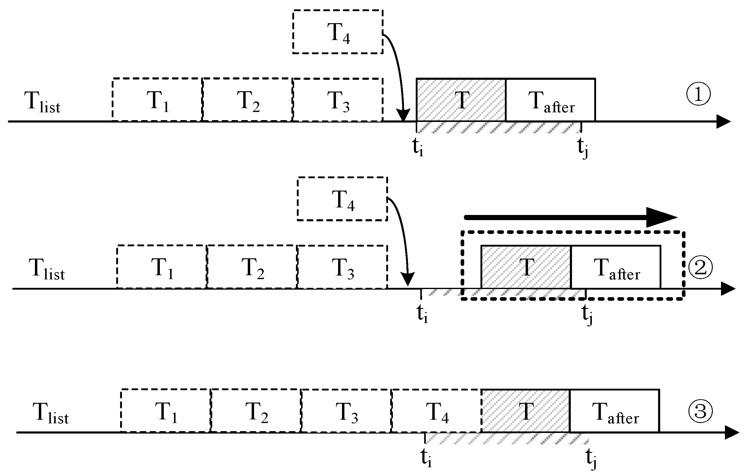
At this point, conflicts may be encountered. For example, task T4 in Figure 5; at this point, there is not enough space in T3 and T for T4 to go through, but T has a corresponding time constraint that must be completed after the moment ti and before the moment tj. If T is allowed to be completed after T4, it may cause logical conflicts.
Therefore, the algorithm lets task T and its related extended tasks move backward and ensure they are within the time windows of ti and tj. The schematic of the move is shown in Figure 5.
Thankfully, the vast majority of actual spacecraft tasks have a large enough time window that failure for time-constrained scheduling is a rare occurrence.
The pseudo-code for spacecraft timing planning is shown in Algorithm 2. The algorithm first initializes the timeline for all APIDs and sets their pointers to zero. In the main loop, the algorithm iterates through each task, obtains the current pointer value based on the task’s APID, checks that the task does not overlap with a task that has an absolute time limit, and adjusts the pointer position accordingly. The task is then added to its corresponding APID timeline. For tasks with absolute time constraints, the algorithm schedules them directly at the specified start time.
| Algorithm 2 Timeline Timing Planning Algorithm |
| Require: task sequence Ensure: Sequences with temporal information
|
4.6. Resource Constraint Planning Method Based on Conflict Elimination
Considering that multiple timelines (i.e., application processes) are allowed to execute related tasks simultaneously during the processing of time constraints, the feasibility of resource allocation must be considered when these tasks are performed simultaneously.
For example, when two payloads expect to downlink image data simultaneously, communication channel occupancy is an issue to consider, i.e., the channel required for downlinking must be smaller than the one owned. When the channel occupancy for the simultaneous execution of tasks exceeds the maximum channels available, the delayed execution of tasks must be considered. A related schematic is shown in Figure 6.
For the sequence of tasks P that has been given temporal information, each of the tasks t in it includes several resources :
for each resource and also for the maximum resource occupancy of the spacecraft, for the spacecraft state at each moment in time,
Therefore, in the face of the resource handling problem of task execution, and considering that the timing and logical planning will not be changed, based on the execution priority of the task, we eliminate the related resource conflicts.
Firstly, we search for the resource occupation of tasks by traversing backward in time. For the set of all tasks occupying resources at a certain instant, the priority of the relevant tasks is set as , and all the tasks in are sorted according to the priority from high to low; then, we obtain
Second, based on the greedy algorithm, the corresponding tasks are selected to be added to the set of tasks to be executed based on the priority from high to low. Third, it traverses backward in time until the entire timeline is traversed. The addition is stopped if a particular item’s resource occupation exceeds the threshold after adding a task. The remaining tasks (including this task) will not be added. At last, it is backward and repaired like in Figure 6 until a particular moment when the resource usage no longer exceeds the threshold.
Figure 6 illustrates that when a resource (V in the figure) is in conflict, the task with lower priority moves backward. T5 in the figure is a vertical extension of T6 and therefore moves backward following T6. Afterward, the tasks on both timelines 2 and 3 undergo a backward change in time due to resource conflicts.
The relevant pseudo-code is in Algorithm 3.
| Algorithm 3 Resource Planning Algorithm |
| Require: Sequences with temporal information Ensure: without resource conflict or failure
|
5. Experimentation
The experiments ignore the actual scenarios and just focus on algorithms, and principle verification of the algorithm is conducted, which includes testing for logic, time, and resource conflict elimination, as well as multi-tasking stress testing. Tests are conducted with the same hardware configuration as in real-world application scenarios. The algorithms related to this research are implemented based on the embedded Linux environment, with Ubuntu 22.03 as the operating system, and the algorithms are developed through C language. The related experiments are carried out directly in the embedded environment.
Relying on the principle of the algorithm, baseline testing is completed with sufficient resources and no time constraints to ensure that the algorithm operates appropriately. During the baseline testing, this study generates a series of TOCs and their accompanying CTCT with the help of the Electronic Data Sheet toolchain. In this experiment, the total number of TOCs was specified as five. The test results based on these commands are shown in the following Table 9.
In Table 9, the number of rows in the CTCT refers to the number of rows corresponding to the Command Template Configuration Table when this test case is tested. The more rows there are, the more computationally intensive the algorithm is. The number of timelines refers to the cumulative number of timelines (i.e., APIDs) occupied by all Primitive-level Commands involved in this test case.
For each test case, all the parameters and Primitive-level Commands are input into the CTCT according to the format described in the previous section, and then according to the input TOC, the corresponding results are output to complete the test of the test case.
The table displays the outcomes of 16 individual test cases, each representing a TOC, every TOC tested 20 times. Due to the algorithm’s inherent randomness, scheduling results can vary with each execution. The above table illustrates that scheduling can be completed quickly, revealing a positive correlation between the CTCT’s row count and execution time.
The scheduling success rate reflects the algorithm’s ability to produce an applicable sequence. Despite limited resources and time constraints, the algorithm consistently achieves successful scheduling, demonstrating its practical applicability.
Second, we conducted tests with varied tasks, time constraints, and limited resources beyond the baseline to validate the algorithm’s efficacy in managing resource and time constraints. In this experiment, the total number of TOCs was specified as five. The test results based on these commands are shown in Table 10 below. All the test cases are based on test cases 1–16, to which relevant time constraints and resource constraints are added.
In the table, the time constraints, number of extensions, and resource limit are defined in advance within the CTCT and RSIT before each case test. The tests detailed in the table above involve multiple time and resource constraints. These are also considered for the task’s horizontal and vertical extensions. We stipulate that upon scheduling failure, the algorithm retries until successful. If scheduling keeps failing, at the same time, the spacecraft operation can be controlled by “assertion” (a statement in a program that checks if a condition is true and throws an error if it is not) when the constraints are not satisfied so that even if the planning fails, the robustness and safety of the spacecraft operation will not be affected.
The table suggests the algorithm achieves a high scheduling success rate and can fulfill practical demands. The data further reveal that the algorithm consistently achieves a high scheduling success rate, even under more complex task configurations (for instance, test case 15, which involves a greater number of timelines and task extensions), demonstrating the algorithm’s robust adaptability to complex tasks. In cases of planning failures, the algorithm’s inability to identify a solution meeting all constraints is primarily attributed to its handling of specific stochastic factors. For these cases, the algorithm successfully schedules a second attempt without significant drawbacks.
The algorithm undergoes a stress test designed to assess the impacts of increased data volume on its performance. Some specific test cases amplify the volume of temporal constraints and resource constraints to investigate the algorithm’s responsiveness to enhanced complexities. The test results of the stress test are shown in Table 11 and Figure 7.
The table above presents 10 test cases, identical except for the varying number of time constraints and rows in the CTCT. The time constraints and CTCT rows were significantly increased to facilitate extreme case testing, despite such conditions being rare in practical applications. The test result values were derived from averaging 20 iterations of each use case under specific conditions.
The data from the table indicate that an increase in the CTCT rows leads to a significant rise in the average scheduling time, yet the rate of scheduling success remains mostly stable. Elevated time constraints lower the scheduling success rate due to conflicts between certain stochastic solutions and these constraints. Typically, a viable solution emerges by the second or third attempt at scheduling.
According to the above table and the above figure, it can be noticed that the complexity of the algorithm shows a linear pattern and is related to the number of CTCTs. Therefore, this complexity is able to satisfy the actual applicable scenarios of the spacecraft. Thus, integrating findings from the aforementioned experiments, it emerges that the algorithm is theoretically capable of meeting practical application needs. The subsequent experiments in this paper will focus on considering the deployment and application of the algorithms to real-world problems.
6. Application
To assess TOCs’ application in practical engineering, this study establishes a physical architecture based on the Space–ground Collaborative Management and Control System (SCMCS) [33], as depicted in Figure 8.
The system is primarily engineered to fulfill the requirements for integrated management and control of all spacecrafts within the space–ground interface. Within the system, the Spacecraft Operations Simulation device interfaces with the load manager via the 1553 B bus, facilitating the transmission of control commands and reception of engineering parameters. The load manager gathers simulation data via the RS422 interface, ensuring effective communication with the digital load. The Spacecraft Operations Simulation device and the Control Protocol Engine (GMCPE) interact through file sharing for remote-control and telemetry data exchange while the GMCPE and the Ground Operation and Control System (GOCS) interact with remote-control data and telemetry data through database and file sharing. The system also comprises various components, such as a load manager, Spacecraft Operations Simulation device, and digital load, among others, including Ground-based Management.
In this architecture, the environment and development language of the algorithms are the same as in the experiments. In this system, we link the rotary table and camera as the two basic payloads, enabling the planning system to manage their scheduling via the load manager.
We designed the corresponding Primitive-level Commands based on this system. The Primitive-level Commands target the instantiation of a camera and rotary table. These commands are considered indivisible.
Furthermore, the system incorporates three types of TOCs: payload state management, resource management, and rotary table scheduling, as detailed in Table 12.
In this paper, we take the rotary table load scheduling as an example to evaluate the effectiveness of spacecraft task scheduling.
The rotary table load scheduling task needs to rotate the table to a specific absolute angle, and the desired effect is that no matter what angle the spacecraft is at, it will rotate to the absolute angle after receiving the command. In traditional spacecraft operations, task execution typically requires sequentially sending a series of Primitive-level Commands programmed by onboard computers. Contrastingly, the method proposed in this study only needs to send a TOC to specify the target, and the spacecraft can autonomously generate an executable sequence based on the current environment without human injection.
To evaluate the algorithm’s accuracy, we devised an experiment using the rotary table payload scheduling task, identified by Task ID 0 × 65, where diverse parameters were input to produce an executable sequence. The rotary table displays three distinct sequences generated for varied initial states in the experiments. The specific generated sequences are shown in Table 13.
In Table 13, the azimuth and pitch angles can be adjusted simultaneously so that the above tasks can be performed simultaneously as two timelines to shorten the execution time of the tasks. The experiments demonstrate that the TOC effectively achieves the spacecraft’s task objectives, facilitating a shift to “objective-driven” capability enhancement.
7. Conclusions
This study introduces the TOC concept, designed to fulfill spacecraft’s specific autonomous operational needs in deep space exploration. Subsequently, we devise a task scheduling strategy using the HTN-T algorithm aligned with this concept. This algorithm facilitates a paradigm shift for spacecraft operation, transitioning from the TOC’s objective-driven to behavior-driven processes. Furthermore, it enables the transformation of the TOC into primitive tasks that are directly executable, thereby producing granular scheduling results that spacecrafts can immediately implement.
In this study, we conduct both principle and application verifications of the HTN-T algorithm. The results demonstrate its high scheduling success rate and operational efficiency within acceptable time limits, effectively addressing autonomous task scheduling challenges for spacecrafts. Therefore, this research is of great significance to support the adaptive scientific exploration of spacecrafts and to improve the intelligent capability of spacecrafts.
This research further explores diverse decomposition strategies for individual TOCs. However, challenges remain in real-world scenarios, particularly in mixed scheduling multiple TOCs and rescheduling these instructions in response to environmental and resource changes. At the same time, the autonomous generation of the TOC on spacecrafts is also a problem that needs to be solved, which is quite important to further improve the autonomy of spacecrafts in the future. Addressing these challenges constitutes the future trajectory and focus of our research.
Author Contributions
Conceptualization, J.Z.; methodology, L.L.; software, J.Z.; validation, J.Z.; writing, J.Z. All authors have read and agreed to the published version of the manuscript.
Funding
This work was supported by China’s Beijing Science and Technology Program, cultivated by the Space Science Laboratory of Beijing Huai rou Comprehensive National Science Center under grant Z201100003520006.
Data Availability Statement
The data presented in this study are available on request from the corresponding author.
Conflicts of Interest
The authors declare no conflicts of interest.
References
- Cordell, G. Theorem Proving by Resolution as a Basis for Question-Answering Systems. Mach. Intell. 1969, 4, 183–205. [Google Scholar]
- John, M. Situations, Actions, and Causal Laws; Comtex Scientific: New York, NY, USA, 1963. [Google Scholar]
- Fikes, R.E.; Nilsson, N.J. Strips: A New Approach to the Application of Theorem Proving to Problem Solving. Artif. Intell. 1971, 2, 189–208. [Google Scholar] [CrossRef]
- Howe, A.; Knoblock, C.; McDermott, I.S.D.; Ram, A.; Veloso, M.; Weld, D.; Sri, D.W.; Barrett, A.; Christianson, D. PDDL—The Planning Domain Definition Language; Technical Report; The AIPS-98 Planning Competition Committee: Pittsburgh, PA, USA, 1998; pp. 1–27. [Google Scholar]
- Steve, C.; Smith, B.; Rabideau, G.; Muscettola, N.; Rajan, K. Automated Planning and Scheduling for Goal-Based Autonomous Spacecraft. IEEE Intell. Syst. Their Appl. 1998, 13, 50–55. [Google Scholar]
- Steve, C.; Sherwood, R.; Tran, D.; Cichy, B.; Rabideau, G.; Castano, R.; Davies, A.; Lee, R.; Mandl, D.; Frye, S. The Eo-1 Autonomous Science Agent. In Proceedings of the Third International Joint Conference on Autonomous Agents and Multiagent Systems—Volume 1, New York, NY, USA, 19–23 July 2004. [Google Scholar]
- Steve, C.; Tran, D.; Rabideau, G.; Schaffer, S.; Mandl, D.; Frye, S. Timeline-Based Space Operations Scheduling with External Constraints. In Proceedings of the International Conference on Automated Planning and Scheduling, Nancy, France, 26–30 October 2020. [Google Scholar]
- Marie-Claire, C.; Pouly, J.; Bensana, E.; Lemaître, M. Testing Spacecraft Autonomy with Agata. In Proceedings of the 9th International Symposium on Artificial Intelligence, Robotics and Automation in Space (ISAIRAS), Los Angeles, CA, USA, 1 January 2008. [Google Scholar]
- Paul, M.; Schwabacher, M.; Dalal, M.; Fry, C. Embedding Temporal Constraints for Coordinated Execution in Habitat Automation. In Proceedings of the International Workshop on Planning and Scheduling for Space, Mountain View, CA, USA, 25–26 March 2013. [Google Scholar]
- Johnston Mark, D. Spike: Ai Scheduling for Nasa’s Hubble Space Telescope. In Proceedings of the Sixth Conference on Artificial Intelligence for Applications, Santa Barbara, CA, USA, 5–9 May 1990. [Google Scholar]
- Jianshen, S.; Zhang, J.; Luo, Y. A Space Station Mission Replanning Method Based on a Deep Reinforcement Learning Algorithm. Manned Spacefl. 2020, 26, 469–476. [Google Scholar]
- Liu, Y. Algorithms and Simulation for Satellite Payload Planning and Scheduling. Master’s Thesis, Chinese Academy of Sciences (Space Science and Application Research Center), Beijing, China, 2004. [Google Scholar]
- Yao, M.; Zhao, M. Autonomous Scheduling Design for Small Satellite Missions Based on Fuzzy Neural Network. J. Astronaut. 2007, 385–388+426. [Google Scholar] [CrossRef]
- Martin, S.F.; Kennedy, B.; Mackey, R.; Troesch, M.; Altenbuchner, C.; Bocchino, R.; Fesq, L.; Hughes, R.; Mirza, F.; Nikora, A. Demonstrations of System-Level Autonomy for Spacecraft. In Proceedings of the 2021 IEEE Aerospace Conference (50100), Big Sky, MT, USA, 6–13 March 2021. [Google Scholar]
- Jun, L.; Zhu, Y.-H.; Luo, Y.-Z.; Zhang, J.-C.; Zhu, H. A Precedence-Rule-Based Heuristic for Satellite Onboard Activity Planning. Acta Astronaut. 2021, 178, 757–772. [Google Scholar]
- Lyu, L. Design a Nd Application Study of Intelligent Flight Software Architecture on Spacecraft. Ph.D. Thesis, University of Chinese Academy of Sciences (National Space Science Center of Chinese Academy of Sciences), Beijing, China, 2019. [Google Scholar]
- Ilche, G.; Aiello, M. An Overview of Hierarchical Task Network Planning. arXiv 2014, arXiv:1403.7426. [Google Scholar]
- De Simone, C.F.; Ferreira, M.G.V.; de Novaes Kucinskis, F. An Extended Htn Language for Onboard Planning and Acting Applied to a Goal-Based Autonomous Satellite. IEEE Aerosp. Electron. Syst. Mag. 2021, 36, 32–50. [Google Scholar]
- Simon, G.; Shaya, E.; Rice, K.; Cooper, S.; Dunham, J.; Champion, J. Xtce: A Standard Xml-Schema for Describing Mission Operations Databases. In Proceedings of the 2004 IEEE Aerospace Conference Proceedings (IEEE Cat. No. 04TH8720) 2004, Big Sky, MT, USA, 6–13 March 2004. [Google Scholar]
- CCSDS. Ccsds 660.0-G-1 Xml Telemetric and Command Exchange (Xtce); CCSDS: Washington, DC, USA, 2007. [Google Scholar]
- ECSS-E-ST-70-41C; ECSS. Telemetry and Telecommand Packet Utilization. European Cooperation for Space Standardization: Noordwijk, The Netherlands, 2016.
- CCSDS. Space Packet Protocol: 133.0-B-2; CCSDS: Washington, DC, USA, 2020. [Google Scholar]
- Maullo, M.J.; Calo, S.B. Policy Management: An Architecture and Approach. In Proceedings of the 1993 IEEE 1st International Workshop on Systems Management 1993, Los Angeles, CA, USA, 14–16 April 1993. [Google Scholar]
- Coelho, C. Comparison of the Ccsds Mission Operations Services with the Packet Utilization Standard Services. Master’s Thesis, Luleå University of Technology, Luleå, Sweden, 2014. [Google Scholar]
- Goldman Robert, P.; Kuter, U. Hierarchical Task Network Planning in Common Lisp: The Case of Shop3. In Proceedings of the ELS 2019, Genova, Switzerland, 1–2 April 2019. [Google Scholar]
- Wilkins, D.E. Using the Sipe-2 Planning System; Artificial Intelligence Center; SRI International: Menlo Park, CA, USA, 1999. [Google Scholar]
- Nau, D.S.; Au, T.-C.; Ilghami, O.; Kuter, U.; Murdock, J.W.; Wu, D.; Yaman, F. Shop2: An Htn Planning System. J. Artif. Intell. Res. 2003, 20, 379–404. [Google Scholar] [CrossRef]
- Kautz, H.; Selman, B. Blackbox: A New Approach to the Application of Theorem Proving to Problem Solving. In Proceedings of the AIPS98 Workshop on Planning as Combinatorial Search 1998, Pittsburgh, PA, USA, 7 June 1998. [Google Scholar]
- Nau, D.; Cao, Y.; Lotem, A.; Munoz-Avila, H. Shop: Simple Hierarchical Ordered Planner. In Proceedings of the 16th International Joint Conference on Artificial Intelligence—Volume 2 1999, Stockholm, Sweden, 31 July–6 August 1999. [Google Scholar]
- Wu, D. Application Research on Spacecraft Based on Htn Planning Technology. Master’s Thesis, University of Chinese Academy of Sciences (National Space Science Center of Chinese Academy of Sciences), Beijing, China, 2019. [Google Scholar]
- Lyu, L.; He, R.; Zhang, J. Application Methods of Spacecraft Electronic Data Sheet. Spacecr. Eng. 2022, 31, 126–131. [Google Scholar]
- Wang, X.; Li, S. Research on Constraint Simplification and Mission Planning Method for Deep Space Explorer. J. Astronaut. 2016, 37, 768–774. [Google Scholar]
- Lu, G.; Lyu, L.; Zhang, J. Design of Data Injection Tool Based on Ccsds Rasds Information Object Modeling Method. Spacecr. Eng. 2023, 32, 90–96. [Google Scholar]
Figure 1.
Methods of applying TOC.

Figure 2.
HTN-T task-scheduling framework.

Figure 3.
The overall schematic of the HTN-T method.

Figure 4.
Horizontal and vertical extension of the timeline.

Figure 5.
Processing of time constraints.

Figure 6.
Resource constraint conflict resolution schematic.

Figure 7.
Line graph of stress test results for the HTN-T algorithm.

Figure 8.
The basic structure of the ground Collaborative Management and Control System.


Table 1.
Space Packet structural components [22].
Table 1.
Space Packet structural components [22].
| Packet Header | Packet Data Field | ||||||
|---|---|---|---|---|---|---|---|
| Packet Secondary Header | User Data Field | ||||||
| Command Packet 1 | Command Packet 2 | …… | Command Packet n | ||||
| Command Packet Header | Command Packet Secondary Header | Packet Data Field | |||||
| 6 octets | Variable | 4 octets | 2 octets | Variable | Variable | Variable | |
| 1-65535 octets | |||||||
Table 2.
The packet-data-field-recommended structure of Task-level Objective Command.
| Packet Data Field | |||||||
|---|---|---|---|---|---|---|---|
| Task ID | Conditional Parameters | ||||||
| Number of Condition Parameters | Parameter 1 | …… | Parameter N | ||||
| Physical Scalar Type | Numeric Type | Length | Value | ||||
| 1 octet | 1 octet | 1 octet | 1 octet | 1 octet | Variable | Variable | |
Table 3.
Physical Scalar Type.
| ID | Physical Scalar Type | Value |
|---|---|---|
| 1 | Prerequisite | 00 |
| 2 | Parameter | 01 |
| 3 | Monitoring item | 11 |
Table 4.
The packet-data-field instance of Task-level Objective Command.
| Packet Data Field | |||||||||
|---|---|---|---|---|---|---|---|---|---|
| Task ID | Conditional Parameters | ||||||||
| Number of Condition Parameters | Parameter 1 (Azimuth) | Parameter 2 (Pitch Angle) | |||||||
| Physical Scalar Type | Numeric Type | Length | Value | Physical Scalar Type | Numeric Type | Length | Value | ||
| 1 ocete | 1 ocete | 1 ocete | 1 ocete | 1 ocete | 1 ocete | 1 ocete | 1 ocete | 1 ocete | 1 ocete |
| 10000001 | 00000010 | 00000001 | 00000010 | 00000001 | 00011110 | 00000001 | 00000010 | 00000001 | 00111100 |
Table 5.
Command Template Configuration Table information and interpretations.
| Name | Interpretations |
|---|---|
| TOC ID | Task-level Objective Command Unique Identifier |
| Task Level | Defines the level of the task |
| Task Priority | Defines the priority and order of execution of tasks |
| Length of mandate | Defines a range of start and end times for task execution |
| Decomposing Task Information | Defines how tasks are broken down |
| Precondition Information | Defines the preconditions for starting this task |
| Resource information | Defines resource consumption information for this task |
| Load module | Defines the name of the program module that needs to be loaded for this task |
| Command or macro sequence contents | Defines the specific encoding of this command |
Table 6.
The format of Decomposing Task Information Column.
| Number of Disaggregated Task Information N | Task 1 Information | Task 2 Information | … | Task M Information | |
|---|---|---|---|---|---|
| Command Template ID | Parameter Calculation Method | ||||
| 8 bit | 8 bit | 8 bit | (n × 16) bit | … | (40 + n × 16) bit |
Table 7.
The recommended format of Precondition Information Description Column.
| Number of Preconditions | Precondition 1 | Prerequisite 2 | … | Prerequisite n | |||
|---|---|---|---|---|---|---|---|
| ID | Operator | Type | Value | ||||
| 8 bit | 8 bit | 8 bit | 8 bit | 8 bit | (n × 32)bit | … | (n × 32)bit |
Table 8.
The recommended format of Resource Status Information Sheet.
| Status Item ID | Status Item Datatype | Status Entry Operator | Status Item Value |
|---|---|---|---|
| 8 bit | 8 bit | 8 bit | 8 bit |
Table 9.
Baseline test results for the HTN-T algorithm.
| Use Case Number | Number of Rows in the CTCT | Number of Timelines | Average Scheduling Time (ms) |
|---|---|---|---|
| Test Case 1 | 9 | 2 | 875 |
| Test Case 2 | 9 | 4 | 887 |
| Test Case 3 | 10 | 2 | 966 |
| Test Case 4 | 10 | 4 | 1004 |
| Test Case 5 | 11 | 2 | 1035 |
| Test Case 6 | 11 | 4 | 1066 |
| Test Case 7 | 12 | 2 | 1103 |
| Test Case 8 | 12 | 4 | 1077 |
| Test Case 9 | 13 | 2 | 1214 |
| Test Case 10 | 13 | 4 | 1298 |
| Test Case 11 | 14 | 2 | 1326 |
| Test Case 12 | 14 | 4 | 1401 |
| Test Case 13 | 15 | 2 | 1405 |
| Test Case 14 | 15 | 4 | 1519 |
| Test Case 15 | 16 | 2 | 1569 |
| Test Case 16 | 16 | 4 | 1586 |
Table 10.
Test results of constraint handling for the HTN-T algorithm.
| Use Case Number | Based on Case Number | Number of Rows in the CTCT | Number of Timelines | Time Constraints | Number of Extensions | Resource Limit | Average Scheduling Time (ms) | Scheduling Success Percentage (%) | Scheduling Time Percentage Increase (%) | Maximum Number of Scheduling Sessions |
|---|---|---|---|---|---|---|---|---|---|---|
| Test Case 17 | Test Case 1 | 9 | 2 | 1 | 1 | 1 | 886 | 100% | 1.26% | 1 |
| Test Case 18 | Test Case 2 | 9 | 4 | 2 | 2 | 2 | 924 | 100% | 4.17% | 1 |
| Test Case 19 | Test Case 3 | 10 | 2 | 1 | 1 | 1 | 1034 | 100% | 7.04% | 1 |
| Test Case 20 | Test Case 4 | 10 | 4 | 2 | 2 | 2 | 1098 | 100% | 9.36% | 1 |
| Test Case 21 | Test Case 5 | 11 | 2 | 1 | 1 | 1 | 1115 | 100% | 7.73% | 1 |
| Test Case 22 | Test Case 6 | 11 | 4 | 2 | 2 | 2 | 1089 | 100% | 2.16% | 1 |
| Test Case 23 | Test Case 7 | 12 | 2 | 1 | 1 | 1 | 1130 | 100% | 2.45% | 1 |
| Test Case 24 | Test Case 8 | 12 | 4 | 2 | 2 | 2 | 1114 | 100% | 3.44% | 1 |
| Test Case 25 | Test Case 9 | 13 | 2 | 1 | 1 | 1 | 1287 | 100% | 6.01% | 1 |
| Test Case 26 | Test Case 10 | 13 | 4 | 2 | 2 | 2 | 1375 | 100% | 5.93% | 1 |
| Test Case 27 | Test Case 11 | 14 | 2 | 1 | 1 | 1 | 1357 | 100% | 2.34% | 1 |
| Test Case 28 | Test Case 12 | 14 | 4 | 2 | 2 | 2 | 1451 | 95% | 3.57% | 2 |
| Test Case 29 | Test Case 13 | 15 | 2 | 1 | 1 | 1 | 1409 | 100% | 0.28% | 1 |
| Test Case 30 | Test Case 14 | 15 | 4 | 2 | 2 | 2 | 1570 | 95% | 3.36% | 2 |
| Test Case 31 | Test Case 15 | 16 | 2 | 1 | 1 | 1 | 1620 | 95% | 3.25% | 2 |
| Test Case 32 | Test Case 16 | 16 | 4 | 2 | 2 | 2 | 1652 | 95% | 4.16% | 2 |
Table 11.
Stress test results for the HTN-T algorithm.
| Number of Time Constraints | 0 | 2 | 4 | 6 | 8 | ||||||
|---|---|---|---|---|---|---|---|---|---|---|---|
| Case Number | Task Configuration Information Table Rows | Average Scheduling Time (ms) | Scheduling Success Rate (%) | Average Scheduling Time (ms) | Scheduling Success Rate (%) | Average Scheduling Time (ms) | Scheduling Success Rate (%) | Average Scheduling Time (ms) | Scheduling Success Rate (%) | Average Scheduling Time (ms) | Scheduling Success Rate (%) |
| Test Case 33 | 9 | 1311 | 100% | 1356 | 100% | 1395 | 100% | 1412 | 100% | 1509 | 100% |
| Test Case 34 | 11 | 1413 | 100% | 1443 | 100% | 1477 | 100% | 1497 | 100% | 1534 | 100% |
| Test Case 35 | 13 | 1553 | 100% | 1594 | 100% | 1623 | 100% | 1678 | 100% | 1812 | 100% |
| Test Case 36 | 15 | 1685 | 100% | 1712 | 100% | 1756 | 100% | 1794 | 100% | 1893 | 100% |
| Test Case 37 | 17 | 1787 | 100% | 1903 | 100% | 1955 | 90% | 2008 | 90% | 2079 | 90% |
| Test Case 38 | 19 | 1902 | 100% | 1995 | 100% | 2038 | 100% | 2065 | 100% | 2101 | 100% |
| Test Case 39 | 21 | 1987 | 100% | 2045 | 100% | 2079 | 100% | 2123 | 100% | 2209 | 100% |
| Test Case 40 | 23 | 2033 | 100% | 2089 | 100% | 2150 | 100% | 2193 | 100% | 2302 | 100% |
| Test Case 41 | 25 | 2353 | 100% | 2467 | 100% | 2531 | 100% | 2624 | 100% | 2755 | 90% |
| Test Case 42 | 27 | 2477 | 100% | 2586 | 100% | 2779 | 100% | 2813 | 100% | 2835 | 100% |
| Test Case 43 | 29 | 2677 | 100% | 2753 | 95% | 2802 | 100% | 2953 | 95% | 3011 | 85% |
| … | … | … | … | … | … | … | … | … | … | … | … |
| Test Case 53 | 49 | 4165 | 100% | 4436 | 100% | 4799 | 90% | 4907 | 90% | 5202 | 80% |
Table 12.
TOC for SCMCS.
| Command Name | Command Meaning | ID | Number of Parameters | Parameter 1 | Parameter 2 | Parameter 3 | |
|---|---|---|---|---|---|---|---|
| 1 | Payload Status Management | Sending a command to change the execution state | 0 × 67 | 0 | - | - | - |
| 2 | Payload Resource Management | Execute the rotary table rotation command when the load voltage, temperature, and storage reach a certain value. | 0 × 66 | 3 | Voltage | Temperature | Storage |
| 3 | Rotary table load scheduling | Execute the rotary table command. | 0 × 65 | 2 | Azimuth | Pitch angle | - |
Table 13.
Correspondence between different parameters and generated command sequences.
| No. | 1 | 2 | 3 |
|---|---|---|---|
| Initial azimuth | 80 | 60 | 140 |
| Initial pitch angle | 20 | 85 | 30 |
| TOC and objectives | 0 × 65 Azimuth angle 30 degrees Pitch angle 30 degrees | 0 × 65 Azimuth angle 30 degrees Pitch angle 30 degrees | 0 × 65 Azimuth angle 30 degrees Pitch angle 30 degrees |
| Command sequence and time code | 005 azimuth rotary table load on 010 azimuth rotary table load turntable reverse by 20 degrees 010 pitch rotary table load—forward rotation 015 azimuth rotary table load turntable reverse by 20 degrees 020 pitch rotary table load -rotation stop 025 azimuth rotary table load—reverse rotation 035 azimuth rotary table load rotation stop 045 azimuth rotary table load shutdown 050 pitch rotary table load on 055 pitch rotary table load shutdown | 005 azimuth rotary table load on 010 azimuth rotary table load turntable reverse by 20 degrees 010 pitch rotary table load turntable reverse by 20 degrees 020 azimuth rotary table load—reverse rotation 020 pitch rotary table load turntable reverse by 20 degrees 030 azimuth rotary table load rotation stop 030 pitch rotary table load—reverse rotation 040 azimuth rotary table load shutdown 040 pitch rotary table load -rotation stop 050 pitch rotary table load on 055 pitch rotary table load shutdown | 005 azimuth rotary table load on 010 azimuth rotary table load turntable reverse by 20 degrees 020 azimuth rotary table load turntable reverse by 20 degrees 030 azimuth rotary table load turntable reverse by 20 degrees 040 azimuth rotary table load turntable reverse by 20 degrees 050 azimuth rotary table load turntable reverse by 20 degrees 055 azimuth rotary table load—reverse rotation 060 azimuth rotary table load rotation stop 065 azimuth rotary table load shutdown |
| Final state | Azimuth angle 30 degrees Pitch angle 30 degrees | Azimuth angle 30 degrees Pitch angle 30 degrees | Azimuth angle 30 degrees Pitch angle 30 degrees |
Disclaimer/Publisher’s Note: The statements, opinions and data contained in all publications are solely those of the individual author(s) and contributor(s) and not of MDPI and/or the editor(s). MDPI and/or the editor(s) disclaim responsibility for any injury to people or property resulting from any ideas, methods, instructions or products referred to in the content. |
© 2024 by the authors. Licensee MDPI, Basel, Switzerland. This article is an open access article distributed under the terms and conditions of the Creative Commons Attribution (CC BY) license (https://creativecommons.org/licenses/by/4.0/).
Share and Cite
MDPI and ACS Style
Zhang, J.; Lyu, L. A Spacecraft Onboard Autonomous Task Scheduling Method Based on Hierarchical Task Network-Timeline. Aerospace 2024, 11, 350. https://doi.org/10.3390/aerospace11050350
AMA Style
Zhang J, Lyu L. A Spacecraft Onboard Autonomous Task Scheduling Method Based on Hierarchical Task Network-Timeline. Aerospace. 2024; 11(5):350. https://doi.org/10.3390/aerospace11050350
Chicago/Turabian StyleZhang, Junwei, and Liangqing Lyu. 2024. "A Spacecraft Onboard Autonomous Task Scheduling Method Based on Hierarchical Task Network-Timeline" Aerospace 11, no. 5: 350. https://doi.org/10.3390/aerospace11050350
Note that from the first issue of 2016, this journal uses article numbers instead of page numbers. See further details here.