
A Novel Explicit Canonical Dynamic Modeling Method for Multi-Rigid-Body Mechanisms Considering Joint Friction
College of Astronautics, Nanjing University of Aeronautics and Astronautics, Nanjing 211106, China
*
Author to whom correspondence should be addressed.
Aerospace 2024, 11(5), 368; https://doi.org/10.3390/aerospace11050368
Submission received: 17 March 2024
/
Revised: 1 May 2024
/
Accepted: 3 May 2024
/
Published: 6 May 2024
Abstract
:Friction is an inevitable phenomenon in mechanical systems that affects the dynamic characteristics of systems. To reduce the modeling complexity of complex multi-rigid-body mechanisms, a novel explicit canonical dynamic modeling method considering joint friction is proposed. Based on the explicit dynamic modeling theory that we have proposed, the solution of the constraint force required by the joint friction modeling of multi-rigid-body mechanisms is derived and improved, which greatly simplifies the solution of the constraint force. According to the obtained explicit expression of the constraint force equations, two joint friction models of the Coulomb–viscous effect and Stribeck effect are derived in analytical form. Moreover, the Stribeck effect of the joint is experimentally analyzed. A five-axis tree-chain mechanism and a three-loop closed-chain mechanism are chosen to demonstrate the method and compared with ADAMS software. Moreover, the proposed model is analyzed and compared with other methods.
1. Introduction
For multi-rigid-body mechanisms in real working environments, joint friction is an inevitable phenomenon and can cause problems, such as limit cycle oscillation and stick–slip motion [1,2]. Many existing studies regard joint friction as an external disturbance, and researchers have reduced its impact on system control performance by enhancin1g the robustness of system controllers [3]. However, the nonlinear characteristics of joint friction, such as hysteresis and undesired stick–slip motion, are particularly obvious when the mechanism is moving at low or high speeds, which leads to a high gain control loop and limited control precision of the system and, thus, affects the smoothness of the mechanism [3,4,5,6]. Accurate modeling of the joint friction of multi-rigid-body mechanisms and feedforward control compensation can improve the motion accuracy and smoothness of mechanisms, so the dynamic modeling of multi-rigid-body mechanisms considering joint friction has attracted the attention of many scholars [7,8,9,10]. Complex multi-rigid-body mechanisms have many motion components and complex structures, which make dynamic modeling considering joint friction difficult [11]. In many existing studies of complex multi-rigid-body dynamic modeling considering joint friction, the joint friction modeling either oversimplifies the joint dynamic expression or adopts planar joint models, which will make the calculated friction difficult to reflect the actual situation [1,2,3]. Therefore, it is important to establish the accurate expression of the joint friction model of complex multi-rigid-body mechanisms.
The complete dynamic model of multi-rigid-body mechanisms considering joint friction in real work usually contains two parts: one is the inertial dynamics caused by link motions, and the other is about the joint friction [12]. In terms of the inertial dynamic modeling of multi-rigid-body mechanisms, the methods can be divided into recursive implicit modeling based on the Newton–Euler equation and iterative explicit modeling based on the Lagrangian equation [13,14,15,16]. The recursive implicit modeling method is popular because of its excellent computational efficiency. For example, Walker and Orin [17] proposed the composite rigid body algorithm (CRBA); Featherstone [18] proposed the articulated body algorithm (ABA), which improved the CRBA. Compared with the recursive implicit modeling method, the advantage of the iterative explicit modeling method is that it can systematically generate the closed form of the dynamic equations, and the method can also explicitly analyze each dynamic effect according to the model [13]. This iterative explicit modeling method that can provide direct insight into the model structure is more conducive to the design of the control system; for example, to compensate gravity loads, the explicit model of gravity can be directly used [3,13]. Uicker [19] first proposed the pseudo-inertial matrix method to further derive the Lagrangian equation, simplifying energy analysis and derivative operations. Li [20] further derived the Uicker equation and eliminated some partial derivative terms. Siciliano [21] proposed the generalized momentum method to obtain explicit dynamic equations, but this method still requires a large number of calculations on intermediate variables, such as Jacobian matrices and Christoffel symbols. To solve the problems of the existing explicit modeling methods, we recently proposed an explicit canonical dynamic modeling method [22,23], which can directly obtain the final dynamic expressions of multi-rigid-body mechanisms.
Regarding the joint friction modeling of multi-rigid-body mechanisms, there is currently no model that can fully and accurately describe all the phenomena caused by friction [12] because joint friction is affected by many factors, such as the load, speed, and even the temperature [24,25,26]. The friction model used in engineering often involves a tradeoff between simplicity and accuracy [27]. The linear friction model composed of Coulomb friction and viscous friction is still widely used because this friction model is simple and can also describe the main contribution of the joint friction in many cases [12]. However, this linear friction model cannot describe the highly nonlinear characteristics of joint friction at low speeds [1,5]. To solve this problem, the nonlinear model considering the Stribeck effect is adopted in the joint friction modeling of multi-rigid-body precision mechanisms [28]. A widely used friction model is proposed by Bo and Pavelescu [29], which takes into account the Coulomb, viscous, stiction, and Stribeck friction effects. However, this model is a velocity-based model that does not capture the micro-slip phenomenon and is not continuous. To capture the micro-slip phenomenon, several friction models based on the concept of bristle deflection have been proposed, such as the bristle model [30], the LuGre model [31], and the Gonthier model [32], among others [33,34]. However, these models become more complex and often discontinuous because of additional state variables associated with bristle deflection. Recently, Brown and McPhee [35] proposed an advanced simple velocity-based continuous friction model and compared it with common continuous friction models, such as those by Andersson et al. [36], Hollars [37], and Specker et al. [38].
According to whether the kinematic chains of multi-rigid-body mechanisms are closed, multi-rigid-body mechanisms can be divided into open-chain mechanisms (including single-chain mechanisms and tree-chain mechanisms) and closed-chain mechanisms (also called parallel mechanisms) [39]. The inherent motion constraints of the closed chain complicate dynamics research [40,41], considering that joint friction strengthens the coupling degree of the closed-chain dynamic model and increases the difficulty of such research [42]. Ryu [43] adopted the Coulomb friction model for the joint friction modeling of a parallel 6-degree-of-freedom (DOF) manipulator. Shang [44] used the Coulomb friction model, viscous friction model, and Stribeck friction model for the joint friction modeling of a 2-DOF planar parallel robot. However, these studies oversimplify or estimate the friction model, which will lead to the loss of the accuracy of the friction model and the lag of the friction compensation control [1,2,3]. Joint friction models with calculated constraint forces have more complete expressions [3]. The motion components of complex multi-rigid-body mechanisms are numerous, and each joint has dynamic coupling, so the calculation of joint constraint forces is difficult [11]. Shiau [45] derived the joint constraint forces of a parallel mechanism based on the Newton–Euler method and constructed a Coulomb friction model. Yuan [46] derived the joint constraint forces of a 3-PRS parallel robot and constructed a LuGre friction model. References [1,2] used the single direction recursive construction method to calculate the joint constraint forces of a space robot and constructed a Coulomb friction model, a Stribeck friction model, and a LuGre friction model. However, these methods have not obtained the analytical expression of the joint constraint forces. Haug [47] derived the exact analytical expressions of the joint constraint forces of revolute, cylindrical, and translational joints in reference point coordinates with Euler parameters. Verulkar [48] recently completely calculated the joint normal force using the fully implicit multi-body dynamic formulation and studied the Brown–McPhee friction model. Zhao [3] recently proposed an advanced closed-chain dynamic modeling method considering joint friction after expanding the Udwadia–Kalaba equation. However, Zhao’s method has the problem for requiring a large number of intermediate variables to be solved.
In this paper, a novel modeling approach based on explicit dynamic modeling theory (created and developed in [22,23,49,50,51,52]) for multi-rigid-body mechanisms with joint friction is presented. Based on the explicit dynamic modeling theory we have proposed, the constraint force equations required for joint friction modeling are established and improved, and two joint friction models are developed. According to the derived joint friction model, complete dynamic models of tree-chain mechanisms and closed-chain mechanisms considering joint friction are established and solved. The remainder of this paper is organized as follows: In Section 2, we briefly introduce the explicit canonical dynamic modeling theory that we have proposed, which is an ideal dynamic modeling method for multi-rigid-body mechanisms without considering joint friction. In Section 3, using the explicit dynamic modeling theory, we derive and improve the constraint force required for joint friction modeling of multi-rigid-body mechanisms and establish two joint friction models considering the Coulomb–viscous effect and Stribeck effect, in which the Stribeck effect of the joint is experimentally analyzed. In Section 4, we analyze the establishment and solution of the complete dynamic model of tree-chain mechanisms and closed-chain mechanisms considering joint friction. In Section 5, we illustrate and analyze the proposed modeling method by taking a five-axis tree-chain mechanism and a three-loop closed-chain mechanism as examples. The results are discussed in Section 6, and the conclusions are provided in Section 7.
2. Explicit Canonical Dynamic Modeling Theory
This section mainly gives a brief introduction to the explicit canonical dynamic modeling theory that has been proposed and provides a theoretical basis for the following dynamic modeling considering joint friction. Because dynamics are an extension of kinematics [53], in this section, we first introduce kinematic modeling based on the axis-invariant and then introduce the ideal dynamic modeling of tree-chain mechanisms and closed-chain mechanisms.
2.1. Kinematic Modeling
The topological structure analysis and the establishment of a reference coordinate system are the basis for the kinematic modeling of multi-rigid-body mechanisms [18].
From the perspective of the topological structure, multi-rigid-body mechanisms are composed of links and joints (also known as kinematic pairs) [18]. Therefore, the topological graphs of multi-rigid-body mechanisms are usually composed of nodes representing the links (except the root node) and arcs representing the joints [18]. For the convenience of the analysis, the root node of the topology of multi-rigid-body mechanisms is usually numbered as 0, and the remaining nodes representing the links are numbered from 1 to n according to the actual corresponding position of the links in multi-rigid-body mechanisms. The joint types of the topological graphs of multi-rigid-body mechanisms include two types of single-degree-of-freedom kinematic pairs, namely, the revolute pair and the prismatic pair, denoted by and , respectively. To obtain the spanning tree mechanism corresponding to the closed-chain mechanism, some joints of the closed-chain mechanism need to be cut [18]. We take the spanning tree mechanism and its topological analysis, corresponding to the closed-chain mechanism shown in Figure 1, as an example, where represents the kinematic pair composed of the parent Link () and the child link (l). In addition, unless otherwise specified, the rest of the symbols used in this article are shown in Table 1. All the vectors and matrices used in the formulae in this paper are shown in bold italics.
To improve the calibration accuracy of the structural parameters of multi-body mechanisms and better control multi-body mechanisms, we propose a natural reference system establishment method based on the axis-invariant [51]. A schematic and the natural reference system of the 6-DOF manipulator built in our laboratory are shown in Figure 2. The natural inertial reference frame () is first established with the ground as the reference, and the base natural reference frame () and joint natural reference frame () are subsequently established according to the principle that the initial axis directions of the base natural reference system and each joint natural reference system are consistent with the axis direction of the inertial natural reference system. The axis-invariant () is defined as the motion axis vector direction of joint l. The reason this is called the axis-invariant is that it has a radial reference direction with zero rotation, and it can be used to describe the rotation transformation matrix without establishing a non-root-linked framework, which can greatly simplify the workload.
The axis-invariants () of the revolute joint and the prismatic joint are shown in Figure 3. As shown in Figure 3, with as the reference axis, the rotational vector () of the rotating joint and the translational vector () of the prismatic joint can be expressed as follows [22]:
The rotation transformation matrix () based on the axis-invariant can be expressed as follows [22]:
According to the transitivity of kinematic chains in multibody systems, the iterative kinematic equations of multi-joint series based on the axis-invariant can be expressed as follows [22]:
where the left superscript “i |” of the vector represents the projection of the vector under the inertial reference frame ().
By taking the first derivative and second derivative of Equations (5) and (6), the iterative velocity and iterative acceleration of multi-joint kinematic chain () can be expressed as follows [22]:
2.2. Ideal Dynamic Modeling of Tree-Chain Mechanisms without Considering Joint Friction
The explicit iterative dynamic modeling method based on the Lagrangian equation is widely used because it simplifies the operation of the model and is very beneficial to the design of the control system [19,20,21]. The Lagrangian multi-rigid-body dynamic equation based on the axis-invariant is expressed as follows [22,23]:
where
The explicit expression of partial derivative equations can eliminate the partial derivative operations in the Lagrangian equation. The iterative partial derivative equations based on the axis-invariant are expressed as follows [22,23]:
The ideal dynamic equation of the m-DOF tree-chain mechanisms without joint friction can be expressed as follows:
where is an m × m symmetric inertia matrix, is an m × 1 joint generalized acceleration vector, is an m × 1 bias force vector, and is an m × 1 joint-generalized driving-force vector.
Substituting Equations (1)–(10) and (12) into Equation (11), removing redundant items, and referring to Equation (16), the explicit canonical dynamic expression of joint u of the tree-chain multi-rigid-body mechanisms based on the axis-invariant can be obtained as follows [22,23]:
where and are 3 × 3 inertia matrices for revolute and prismatic pairs, respectively, and and are 3D bias force vectors for revolute and prismatic pairs, respectively,
2.3. Ideal Dynamic Modeling of Closed-Chain Mechanisms without Considering Joint Friction
The ideal dynamic equation of closed-chain mechanisms corresponding to the m-DOF spanning tree without joint friction can be expressed as follows:
where is the m × 1 joint-generalized external force vector, which mimics the effect of the constraint force at closed-loop joints that are cut on other joints.
To improve the modeling efficiency of closed-chain dynamics, we have proposed an explicit canonical dynamic modeling method for closed chains [52]. The diagram of the spanning tree chain corresponding to the single-loop closed chain shown in Figure 4 is taken as an example. and denote the constraint and reaction forces at cut joints, respectively. denotes the closed-loop joints that are cut.
3. Joint Friction Modeling of Multi-Rigid-Body Mechanisms
3.1. Solution of the Joint Constraint Force
The two arbitrary orthogonal constraint axes that are orthogonal to the motion axis (u) of the kinematic pair () are denoted as and . If the constraint axis vectors corresponding to the two arbitrary orthogonal constraint axes ( and ) are denoted as and , respectively, then the following expressions can be obtained:
For the constraint axis () without power loss, if the magnitude of the constraint torque of the revolute joint on the constraint axis () and the magnitude of the constraint force of the prismatic joint on the constraint axis () are denoted as and then the following expressions can be obtained:
If the constraint torque vector of the revolute joint and the constraint force vector of the prismatic joint corresponding to the constraint axis () are denoted as and , respectively, then the following expressions can be obtained:
Similarly, for the constraint axis () without power loss, if the magnitude of the constraint torque of the revolute joint on the constraint axis () and the magnitude of the constraint force of the prismatic joint on constraint axis () are denoted as and , respectively, then the following expressions can be obtained:
If the constraint torque vector of the revolute joint and the constraint force vector of the prismatic joint corresponding to the constraint axis () are denoted as and , respectively, then the following expressions can be obtained:
According to Equations (28), (30), and (32), we can obtain the following expressions:
Equation (33) shows that there is a natural orthogonal complementary relationship between the axis vector of the motion axis and the constraint force or torque of the constraint axis. Therefore, for joint u of multi-rigid-body mechanisms, if the constraint torque vector of the revolute joint and the constraint force vector of the prismatic joint are denoted as and , respectively, then the following expressions can be obtained:
According to Equations (30) and (32), Equation (34) can be expressed as follows:
For joint u in multi-rigid-body mechanisms, if the magnitude of the constraint torque vector () of the revolute joint and the magnitude of the constraint force vector () of the prismatic joint are denoted as and , respectively, then the following expressions can be obtained:
3.2. Improvement of the Joint Constraint Force Solution Method
In this section, a 3D force screw is proposed to improve the solution method of the joint constraint force proposed in the previous section. To better explain and use the 3D force screw, the 3D motion screw is first analyzed.
3.2.1. 3D Motion Screw
The translation and rotation of a multi-axis system (also known as a multi-body system) in the same axis direction are called screw motion. The screw motion vector, only considered in the three-dimensional vector space, is called the 3D screw motion vector.
In contrast to the traditional Cartesian coordinate system, which consists of three orthogonal and copoint axes, the natural coordinate system has only one parameterized 3D reference axis. Taking the 3D motion screw in Figure 5 as an example, vector is given, and the first-order motion screw axis can be determined by vector and the axis-invariant (). The first-order motion screw axis is orthogonal to the axis-invariant () and vector (). Therefore, the first-order motion screw axis corresponds to . Similarly, the second-order motion screw axis, the third-order motion screw axis, and the fourth-order motion screw axis, with the first-order motion screw axis rotated counterclockwise at 90°, 180°, and 270° correspond to , , and , respectively. The direction of the fourth-order motion screw axis is exactly the opposite to that of the second-order motion screw axis, so the fourth-order motion screw axis also corresponds to .
3.2.2. 3D Force Screw
Taking the 3D force screw in Figure 6 as an example, is the joint-equivalent generalized resultant force acting on the closed subtree (). As shown in Figure 6, when the axis-invariant () is used as the reference axis, the fourth-order force screw axis is the constraint axis of joint u. Therefore, if the generalized constraint force vector of joint u on the constraint axis, that is, the projection force of on the constraint axis, is denoted by , then the following expressions can be obtained:
According to Equation (37), for different joint types, we can obtain the following equations:
where the expressions of and for the tree-chain system and the closed-chain system are shown in Equation (17) and Equation (25), respectively.
According to Equation (36), the magnitude () of the constraint torque vector of the revolute joint and the magnitude () of the constraint force vector of the prismatic joint in Equation (36) can be re-expressed as follows:
According to the force backward iteration formulas [22], for and of joint u, only the driving force and friction force on the current joint can be regarded as the external force, while the driving force and friction force on the other joints of the closed subtree () can be regarded as the internal force. Therefore, when solving for the constraint force of joint u, the driving force and friction force on the other joints of the closed subtree () do not need to be analyzed.
In contrast to the method based on the traditional Cartesian coordinate system, in which two constraint axes need to be established, only one constraint axis needs to be established in the proposed improved constraint force solution method. Hence, the efficiency of the modeling and solving for joint constraints can be significantly improved. In addition, compared with the 6D spatial operator algebra method, which describes rotation and translation together, the proposed 3D screw method considers only rotation or translation, which reduces the matrix dimensions.
3.3. Friction Model
3.3.1. Coulomb–Viscous Friction Model
The schematics of the Coulomb friction and viscous friction for the revolute joint and prismatic joint are shown in Figure 7. The magnitude of the Coulomb friction torque and the magnitude of the Coulomb friction force of joint u are denoted as and , respectively, and the magnitude of the viscous friction torque and the magnitude of the viscous friction force of joint u are denoted as and , respectively.
The Coulomb friction model corresponding to joint u is expressed as follows:
where is the Coulomb friction coefficient, is the equivalent total normal torque of the revolute joint, and is the equivalent total normal force of the prismatic joint.
The viscous friction model corresponding to joint u is expressed as follows:
where is the viscous friction coefficient.
The magnitude of the joint friction torque and the magnitude of the joint friction force of joint u are denoted as and , respectively. According to Equations (40) and (41), the Coulomb–viscous joint friction model of joint u of the multi-rigid-body mechanism is expressed as follows:
According to Equation (42), calculating the joint friction depends on the acquisition of the equivalent total normal torque () and the equivalent total normal force ().
3.3.2. Analysis of and
The geometric model of the revolute joint and the prismatic joint is shown in Figure 8, where Rn is the friction arm, Rp is the pin radius, Rb is the bending reaction arm, is the magnitude of the constraint torque of the constraint axis of the revolute joint, is the magnitude of the constraint force of the constraint axis of the revolute joint, is the magnitude of the constraint force of the motion axis of the revolute joint, is the magnitude of the constraint force of the constraint axis of the prismatic joint, is the magnitude of the constraint torque of the constraint axis of the prismatic joint, and is the magnitude of the constraint torque of the motion axis of the prismatic joint.
According to Equation (39), the analysis of of the revolute joint and of the prismatic joint has been completed. Next, and of the revolute joint and and of the prismatic joint will be analyzed. The analysis reveals that the keys to solving and of the revolute joint and and of the prismatic joint are obtaining the constraint resultant force of the revolute joint and the constraint resultant torque of the prismatic joint, respectively. According to the explicit canonical dynamic modeling theory [22,23], the calculation of the resultant force and resultant torque of each node in the topological structure of the mechanism follows the principle of force reverse iteration. The resultant force and resultant torque of the current node () can be obtained by summing the initial input parameters of node and the iteration results of the descendant node (). Then, traversing over all the nodes along the backward direction of the closed subtree () can complete the iterative operation of the resultant force and resultant torque of all the nodes. The calculation model of the resultant force and the resultant torque of the different joint types of the multi-rigid-body mechanisms is the same. Therefore, the constraint resultant force () of the revolute joint and the constraint resultant torque () of the prismatic joint can also be iteratively and explicitly calculated using Equations (18)–(22).
According to the 3D force screw, and combined with Figure 6, the constraint force vector () of the revolute joint on the constraint axis and the constraint torque vector () of the prismatic joint on the constraint axis can be expressed as follows:
According to Equation (43), the magnitude () of the constraint force vector of the revolute joint on the constraint axis and the magnitude () of the constraint torque vector of the prismatic joint on the constraint axis can be expressed as follows:
Similarly, according to the 3D force screw, and combined with Figure 6, the constraint force vector () of the revolute joint on the motion axis and the constraint torque vector () of the prismatic joint on the motion axis can be expressed as follows:
According to Equation (45), the magnitude () of the constraint force vector of the revolute joint on the motion axis and the magnitude () of the constraint torque vector of the prismatic joint on the motion axis can be expressed as follows:
Thus far, the analysis and solutions of all the constraint forces and constraint torques of the revolute joint and the prismatic joint have been completed. The equivalent total normal torque () of the revolute joint and the equivalent total normal force () of the prismatic joint can be expressed as follows:
where the expressions of each item can be found in Equations (39), (44), and (46).
3.3.3. Stribeck Friction Model
The nonlinear phenomenon of multi-rigid-body mechanism joints at low speeds is obvious, and the Coulomb–viscous linear joint friction model cannot describe this nonlinear phenomenon well. To better understand the variation in the joint friction of a multi-rigid-body mechanism at low speeds, a constant-speed tracking method was adopted in this paper to conduct experimental research on joint 4 of a 6-DOF manipulator established in our laboratory. The physical diagram of the 6-DOF manipulator is shown in Figure 9. The natural reference frame and axis-invariant of the manipulator are shown in Figure 2.
When testing the friction torque of any joint (u), the remaining joints are locked so that joint u rotates at a certain angle and constant speed, and the input torque () corresponding to joint u at this time is recorded. Then, joint u reverses the same angle, and the input torque () corresponding to joint u at this time is recorded. Because the inertia force of joint u is zero when it rotates at a constant speed and because the centrifugal force and Coriolis force of joint u are also zero when other joints are locked, the uniform rotation of joint u only needs to overcome the influence of the frictional torque () and gravitational torque (). Therefore, the torque of joint u at position can be expressed as follows:
At the same round-trip position (), the gravity torque is the same, and the difference in the joint friction torque of the 6-DOF manipulator in the forward and reverse motions is very small, as follows:
Therefore, according to Equations (48)–(50), we can obtain the following expression:
The variations in the friction torque of joint 4 of the 6-DOF manipulator with respect to the speed are shown in Figure 10. According to Figure 10, it is observed that when the manipulator moves at a low speed at the beginning, the friction decreases with increasing motion speed; that is, it shows the Stribeck effect. Based on the proposed explicit normal force expression in Equation (47), a variety of friction models that can describe the Stribeck effect can be established, such as the Stribeck model [29], LuGre model [31], and the more advanced Brown–McPhee model [35]. Among them, the Stribeck friction model is a traditional friction model, which is not only simple but also common in engineering. This paper intends to use the Stribeck friction model proposed by Bo and Pavelescu [29] to describe the Stribeck effect. Schematics of the Coulomb–viscous friction model and the Stribeck friction model are shown in Figure 11.
According to Figure 11 and the experimental analysis, the Stribeck friction model can better describe the variation in the friction force during low-speed joint motion. The Stribeck joint friction model [29] of joint u of the multi-rigid-body mechanism is expressed as follows:
where is the static friction coefficient, is the Stribeck velocity of the revolute joint, is the Stribeck velocity of the prismatic joint, and the expressions and can be found in Equation (47).
4. Modeling and Solving of the Complete Dynamics of Multi-Rigid-Body Mechanisms
In this section, the complete dynamic modeling of tree-chain multi-rigid-body mechanisms and closed-chain multi-rigid-body mechanisms considering joint friction is analyzed in turn.
4.1. Complete Dynamic Modeling of Tree-Chain Mechanisms Considering Joint Friction
The complete dynamic equation of tree-chain mechanisms with m-DOF considering joint friction can be expressed as follows:
where is an m × 1 joint-generalized friction force vector.
According to Equations (17) and (53), the canonical expression of the complete dynamics of joint u of tree-chain mechanisms can be obtained as follows:
where the expressions of each item can be found in Equations (18)–(22), (38), (42), (47), and (52).
4.2. Complete Dynamic Modeling of Closed-Chain Mechanisms Considering Joint Friction
The complete dynamic equation of closed-chain mechanisms corresponding to the spanning tree with m-DOF considering joint friction can be expressed as follows:
According to Equations (27) and (55), the canonical expression of the complete dynamics of the closed-chain mechanisms in Figure 4 can be obtained as follows:
where the expressions of each item can be found in Equations (18)–(22), (26), (38), (42), (47), and (52).
According to Equations (53)–(56), when solving for friction, closed-chain mechanisms first need to be implemented to solve for the joint-generalized external force and are different from tree-chain mechanisms. The constraint torque of the closed-chain mechanisms considered in this paper is zero at the missing joints, which is the same as that in Zhao’s method [3]. The implementation process of the proposed algorithm for solving the complete dynamic model of multi-rigid-body mechanisms is shown in Algorithm 1.
| Algorithm 1: Dynamic algorithm of multi-rigid-body mechanism considering joint friction. |
| 1: Initialization 2: analyze topological structure of mechanism and establish natural reference systems 3: repeat 4: compute inertia matrices and bias force vectors following Equations (19)–(22) 5: if (single chain or tree chain) 6: compute joint constraint forces and torques following Equations (39), (44), and (46) 7: compute joint normal forces and torques following Equation (47) 8: establish friction model following Equation (42) or Equation (52) 9: compute joint-generalized driving forces following Equation (54) 10: else (closed chain) 11: compute passive joint velocities following Equation (24) 12: compute joint-generalized external forces following Equations (25) and (26) 13: compute joint constraint forces and torques following Equations (39), (44), and (46) 14: compute joint normal forces and torques following Equation (47) 15: establish friction model following Equation (42) or Equation (52) 16: compute active joint-generalized driving forces following Equation (56) 17: until mechanism stops |
5. Case Study
5.1. Five-Axis Tree-Chain Mechanism
The five-axis tree-chain mechanism in Figure 12 is taken as an example. The five active joints of the mechanism correspond to the five degrees of freedom of the mechanism. In the following discussion, a complete dynamic modeling approach and an analysis of the five-axis tree-chain mechanism are provided using the proposed method.
- (1)
- All the joints in the five-axis tree-chain mechanism are revolute joints. The constraint torque vector equations of the mechanism can be obtained according to Equation (36) as follows:
- (2)
- The constraint force vector equations of the mechanism can be obtained according to Equations (43) and (45) as follows:
- (3)
- According to the constraint force and constraint torque calculated using the above equations, the friction models of the five active joints can be obtained. Then, the generalized driving forces of the five active joints can be obtained according to Equation (54) as follows:
A computer program is developed according to the proposed dynamic algorithm to simulate the five-axis tree-chain mechanism. The fourth-order Runge–Kutta (RK4) method is used when the joint acceleration is integrated to solve the joint velocity and joint position. The initial parameters used during the simulation are shown in Table 2. The simulation results for joints 1, 2, and 4 of the mechanism are taken as examples for the analysis. The simulated constraint resultant torque and the simulated constraint resultant force of the three joints are shown in Figure 13 and Figure 14, respectively. To verify the simulation results, the dynamic modeling and solving of the five-axis tree-chain mechanism were carried out using ADAMS software. The constraint torque and constraint force of the three joints solved using ADAMS software are also shown in Figure 13 and Figure 14. It can be seen from Figure 13 and Figure 14 that the values calculated using the proposed method are in good agreement with the values calculated using ADAMS software, which verifies the correctness of the constraint force solution method proposed in this paper. The influence of the joint friction on the dynamics of the mechanism is depicted in Figure 15. In this figure, the values of the driving torque of the three joints of the mechanism without considering friction, considering the Coulomb–viscous friction model, and considering the Stribeck friction model are provided. Observations of Figure 15 indicate that the influence of the joint friction cannot be ignored and should be considered, and the Stribeck friction model can be used to better reflect the nonlinear characteristics of the joint at low speeds.
5.2. Three-Loop Closed-Chain Mechanism
Closed-chain mechanisms have been widely studied in recent years because of their high rigidity, high accuracy, and localized workspace. Figure 16 shows a planar closed-chain mechanism with three closed loops, which has been applied and studied in robotic legs and carpet-scraping devices. As shown in Figure 16, the three-loop closed-chain mechanism has 10 joints and 7 links, of which Joint 1″ is active, and the other joints are passive, and the friction of the passive joints is ignored. To obtain the spanning tree corresponding to the three-loop closed-chain mechanism, three closed-loop joints need to be cut.
As shown in Figure 16, the selected joints of the original system will produce three subsystems after three cuts, and only Subsystem III is determined because Subsystem III has four motion equations and four unknowns. These four unknowns are the four components of the two constraint forces generated by the 2nd- and 3rd-cutting closed-loop joints. Subsystem II is uncertain because it has two motion equations and four unknowns. These four unknowns are the four components of the two constraint forces generated by the 1st- and 2nd-cutting closed-loop joints. Subsystem I is also uncertain because it has one motion equation and three unknowns. These three unknowns are two components of one constraint force generated by the 1st-cutting closed-loop joint and one driving torque. Therefore, when solving for the generalized driving torque of Subsystem I, it is necessary to first solve Subsystem II based on the determined Subsystem III to make it a determined system and to then solve Subsystem I. The following is a complete dynamic modeling and analysis of the mechanism using the proposed method.
- (1)
- The three-loop closed-chain mechanism contains three independent loops. Thus, we can obtain three kinematic constraint equations. The kinematic constraint equations of the mechanism can be obtained according to Equation (24) as follows:
- (2)
- The dynamic equations of Subsystem III can be obtained according to Equation (56) as follows:
- (3)
- The constraint force generated by the 2nd-cutting closed-loop joint can be calculated according to Equation (62). Therefore, Subsystem II becomes determinate. The dynamic equations of Subsystem II can be obtained according to Equation (56) as follows:
- (4)
- According to Equation (63), the constraint force generated by the 1st-cutting closed-loop joint can be calculated so that Subsystem I becomes determinate. The constraint torque vector equations and the constraint force vector equations of the active joint (1″) can be obtained according to Equation (38) as follows:
- (5)
- According to the constraint force and constraint torque calculated using the above equations, the friction model of the active joint (1″) can be obtained. Then, the driving torque of the active joint (1″) can be obtained according to Equation (56) as follows:where matrices , vectors , and vectors in Equations (62)–(65) are defined in Equations (A11)–(A31) in Appendix A.
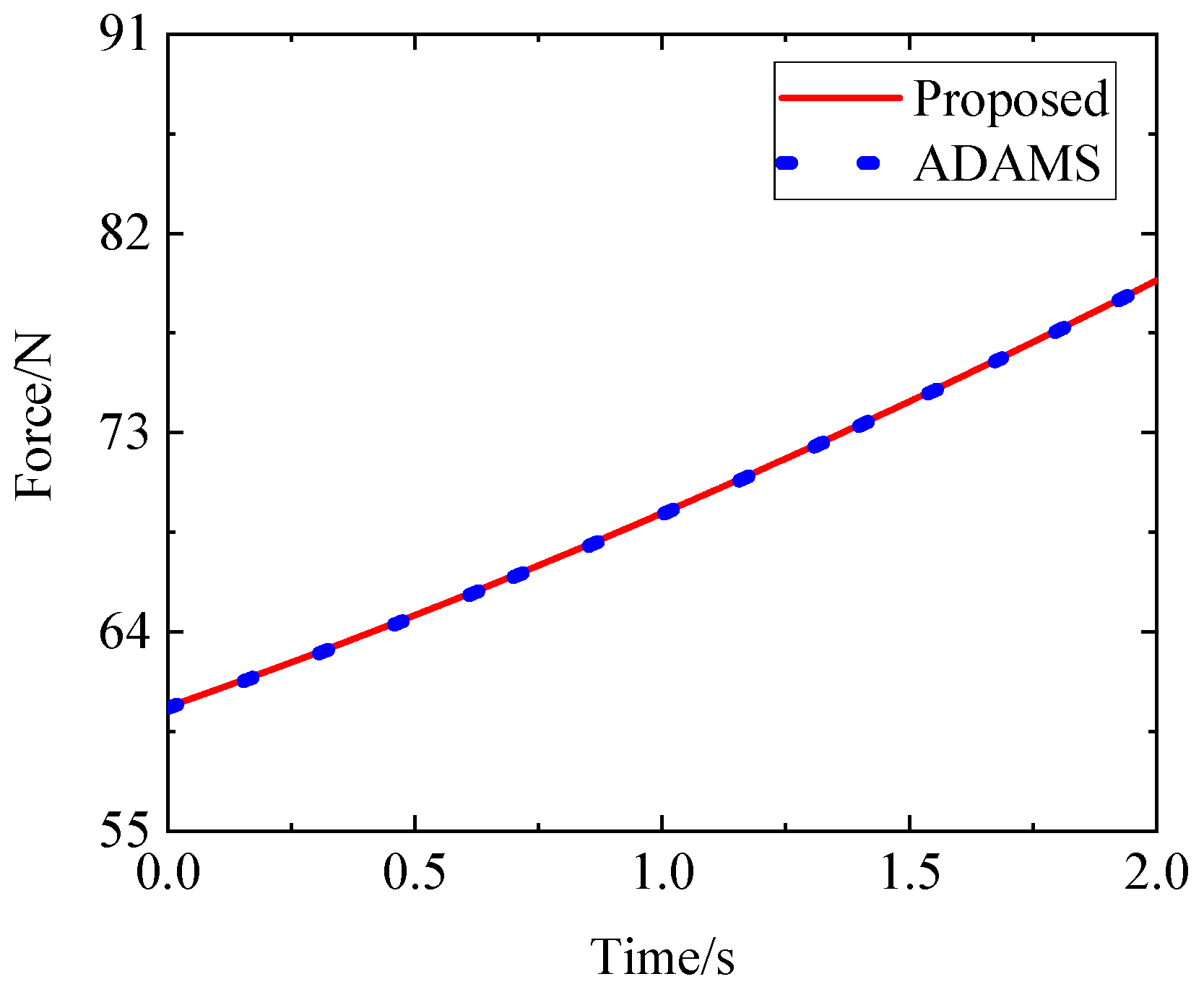
According to the proposed dynamic algorithm, a computer program is developed to simulate the three-loop closed-chain mechanism. The initial parameters used during the simulation are shown in Table 3. The simulated rotation angles of the six passive joints are shown in Figure 17. The simulated constraint forces of the three closed-loop joints are shown in Figure 18. The simulated constraint force of the active joint is shown in Figure 19. To verify the simulation results of the proposed method, the dynamic modeling and solving of the three-loop closed-chain mechanism ware carried out using ADAMS software. The results of the rotation angles of the passive joints, the constraint forces of the closed-loop joints, and the constraint force of the active joint calculated using ADAMS software are also shown in Figure 17, Figure 18, and Figure 19, respectively, which are in good agreement with the values obtained using the method in this paper.
6. Discussion
The advantages of the dynamic modeling method of multi-rigid-body mechanisms considering joint friction, as proposed in this paper, are as follows:
(1) Modeling complexity analysis
The proposed joint constraint force calculation method has the advantage of high modeling efficiency. A comparison between the proposed method and several existing joint constraint force calculation methods is provided as follows:
- ①
- Compared with the traditional Lagrangian calculation method, the proposed method can not only avoid the analysis of the system energy but also avoid the modeling of a large number of intermediate variables and complex partial derivative operations;
- ②
- Compared with the traditional Newton–Euler calculation method, the proposed method can avoid complex force analysis for each joint of the mechanism and a large number of intermediate variable calculations, can explicitly calculate the joint constraint force, and requires fewer constraint force equations;
- ③
(2) Comparison with Zhao’s closed-chain dynamic method
The proposed closed-chain friction modeling method can not only derive the friction dynamic model of the active joints in an analytical form based on the obtained explicit normal force equations but also has the advantage of a relatively simple modeling process.
To obtain the analytical form of the friction model of the active joints of closed-chain mechanisms, Zhao [3] recently proposed an advanced closed-chain dynamic modeling method considering joint friction after extending the Udwadia–Kalaba equation. A comparison between the closed-chain modeling method considering joint friction proposed in this paper and Zhao’s method is provided as follows:
- ①
- For modeling the kinematic constraint equation, two methods can be conducted to determine the explicit expression of the kinematic constraint equations, but Zhao’s method requires complex derivative operations and trigonometric function operations to derive many intermediate variables;
- ②
- For modeling the constraint force equation, both methods provide explicit expressions. However, when Zhao’s method is used to solve the constraint force vectors of different closed-chain mechanisms, complex derivative operations are necessary to deduce multiple intermediate variables. In addition, for Zhao’s method, two constraint axes need to be established when solving for the constraint force;
- ③
- For modeling the inertia matrix and bias force vector, both methods provide explicit expressions, but Zhao’s method uses the traditional Lagrangian method to derive them, which requires complex derivation and partial derivation operations of many intermediate variables.
(3) Fully explicit dynamic Modeling
The fully explicit expression of the dynamic modeling of multi-rigid-body mechanisms considering joint friction is realized. The proposed model realizes the fully explicit expression of the bias force vector (including the Coriolis force vector, centrifugal force vector, and gravity vector), inertia matrix, and generalized friction force vector required for multi-rigid-body dynamic modeling. The independent and explicit expression of the dynamic terms is very beneficial to the motion analysis of the mechanisms. Moreover, compared with other common explicit dynamic modeling methods, the proposed model only needs to determine and replace the relevant parameters to achieve the modeling and solution of the complete dynamics of multi-rigid-body mechanisms considering joint friction, which reduces the difficulty of the engineering implementation.
7. Conclusions
A novel dynamic modeling method for multi-rigid-body mechanisms considering joint friction is proposed in this paper. Based on explicit dynamic modeling theory, the solution of the constraint force required by the key to joint friction modeling is derived and improved. Then, a complete dynamic model of tree chains and closed chains considering joint friction is established. Finally, the proposed method is simulated and analyzed by taking a five-axis tree-chain mechanism and a three-loop closed-chain mechanism as examples. By comparison with the methods of Zhao and others, the proposed method is further analyzed. The main findings of this paper are as follows:
- (1)
- The proposed explicit iterative constraint-force-solving method provides new insights for joint constraint force modeling. The proposed method has the advantages of low computational complexity, high modeling efficiency, and a relatively simple modeling process;
- (2)
- Like Zhao’s closed-chain dynamic method considering joint friction, the proposed method is also based on the derived joint constraint force to obtain the analytical form of the active joint friction model of closed-chain mechanisms, and the derived joint friction and constraint force are also decoupled. However, compared with that of Zhao’s method, the modeling process of the constraint force of the proposed method is simpler;
- (3)
- The proposed multi-rigid-body dynamic model considering joint friction only requires determining and replacing relevant parameters to achieve dynamic modeling and solution, reducing the difficulty of the engineering implementation.
Author Contributions
All the authors contributed to the study’s conception and design. Material preparation, data collection, and analysis were performed by Z.G. and K.W. The first draft of the manuscript was written by Z.G. The manuscript was reviewed and edited by Z.G. and H.J. All authors have read and agreed to the published version of the manuscript.
Funding
This work is supported by the National Natural Science Foundation of China (61673010).
Data Availability Statement
The authors will supply the relevant data in response to reasonable requests.
Conflicts of Interest
The authors have no relevant financial or non-financial conflicts of interest to disclose.
Appendix A
The matrix () elements in Equations (57) and (60) are as follows:
The vector () elements in Equations (57) and (60) are as follows:
The matrix () elements in Equations (62)–(65) are as follows:
The vector () elements in Equations (62)–(65) are as follows:
The vector () elements in Equations (62)–(65) are as follows:
References
- Liu, X.; Li, H.; Wang, J.; Cai, G. Dynamics analysis of flexible space robot with joint friction. Aerosp. Sci. Technol. 2015, 47, 164–176. [Google Scholar] [CrossRef]
- Liu, X.-F.; Li, H.-Q.; Chen, Y.-J.; Cai, G.-P. Dynamics and control of space robot considering joint friction. Acta Astronaut. 2015, 111, 1–18. [Google Scholar] [CrossRef]
- Hui, J.; Pan, M.; Zhao, R.; Luo, L.; Wu, L. The closed-form motion equation of redundant actuation parallel robot with joint friction: An application of the Udwadia–Kalaba approach. Nonlinear Dyn. 2018, 93, 689–703. [Google Scholar] [CrossRef]
- Zhang, Q.; Liu, X.; Cai, G. Dynamics and Control of a Flexible-Link Flexible-Joint Space Robot with Joint Friction. Int. J. Aeronaut. Space Sci. 2020, 22, 415–432. [Google Scholar] [CrossRef]
- Zhao, L.; Zhao, X.-H.; Li, B.; Yang, Y.-W.; Liu, L. Nonlinear friction dynamic modeling and performance analysis of flexible parallel robot. Int. J. Adv. Robot. Syst. 2020, 17. [Google Scholar] [CrossRef]
- Ciliz, M.K. Adaptive control of robot manipulators with neural network based compensation of frictional uncertainties. Robotica 1999, 23, 159–167. [Google Scholar] [CrossRef]
- Grotjahn, M.; Heimann, B.; Abdellatif, H. Identification of Friction and Rigid-Body Dynamics of Parallel Kinematic Structures for Model-Based Control. Multibody Syst. Dyn. 2004, 11, 273–294. [Google Scholar] [CrossRef]
- Karbasizadeh, N.; Zarei, M.; Aflakian, A.; Masouleh, M.T.; Kalhor, A. Experimental dynamic identification and model feed-forward control of Novint Falcon haptic device. Mechatronics 2018, 51, 19–30. [Google Scholar] [CrossRef]
- Jianning, F.; Hanjing, Z.; Wenkang, H. Modeling and Compensation of Non-linear Friction for Spatial Robotic Arm Joint. J. Mech. Transm. 2014, 38, 28–32. [Google Scholar]
- Reynoso-Mora, P.; Chen, W.; Tomizuka, M. A convex relaxation for the time-optimal trajectory planning of robotic manipulators along predetermined geometric paths. Optim. Control Appl. Methods 2016, 37, 1263–1281. [Google Scholar] [CrossRef]
- Guo, F.; Cheng, G.; Pang, Y. Explicit dynamic modeling with joint friction and coupling analysis of a 5-DOF hybrid polishing robot. Mech. Mach. Theory 2021, 167, 104509. [Google Scholar] [CrossRef]
- Wu, J.; Li, W.; Xiong, Z. Identification of robot dynamic model and joint frictions using a baseplate force sensor. Sci. China Technol. Sci. 2021, 65, 1–11. [Google Scholar] [CrossRef]
- Kostic, D.; de Jager, B.; Steinbuch, M. Modeling and Identification for Robot Motion Control, Robotics Automation Handbook; CRC Press: Boca Raton, FL, USA, 2004; Available online: https://research.tue.nl/en/publications/modeling-and-identification-for-robot-motion-control (accessed on 16 March 2024).
- Li, Y. Dynamic Modeling with Joint Friction and Research on the Inertia Coupling Property of a 5-PSS/UPU Parallel Manipulator. JMechE 2019, 55, 43–52. [Google Scholar] [CrossRef]
- Wu, G.; Caro, S.; Bai, S.; Kepler, J. Dynamic modeling and design optimization of a 3-DOF spherical parallel manipulator. Robot. Auton. Syst. 2014, 62, 1377–1386. [Google Scholar] [CrossRef]
- Yen, P.-L.; Lai, C.-C. Dynamic modeling and control of a 3-DOF Cartesian parallel manipulator. Mechatronics 2009, 19, 390–398. [Google Scholar] [CrossRef]
- Walker, M.W.; Orin, D.E. Efficient Dynamic Computer Simulation of Robotic Mechanisms. J. Dyn. Syst. Meas. Control 1982, 104, 205–211. [Google Scholar] [CrossRef]
- Featherstone, R. Rigid Body Dynamics Algorithms; Springer Science and Business Media LLC: Dordrecht, The Netherlands, 2008. [Google Scholar]
- Uicker, J.J. History of Multibody Dynamics in the U.S. J. Comput. Nonlinear Dyn. 2016, 11, 060302. [Google Scholar] [CrossRef]
- Li, C.-J. A New Lagrangian Formulation of Dynamics for Robot Manipulators. J. Dyn. Syst. Meas. Control Eng. Pract. 1989, 111, 559–566. [Google Scholar] [CrossRef]
- Siciliano, B.; Sciavicco, L.; Villani, L. Oriolo, Robotics: Modelling, Planning and Control; Springer: Berlin/Heidelberg, Germany, 2011; Available online: https://link.springer.com/book/10.1007/978-1-84628-642-1 (accessed on 16 March 2024).
- Yang, Y.; Ju, H.; Wang, K. An innovative joint-space dynamic theory for rigid multi-axis system—Part Ⅰ: Fundamental principles. Appl. Math. Model. 2022, 110, 28–44. [Google Scholar] [CrossRef]
- Wang, K.; Ju, H.; Yang, Y. An innovative joint-space dynamic theory for rigid multi-axis system—Part II: Canonical dynamic equations. Appl. Math. Model. 2022, 110, 475–492. [Google Scholar] [CrossRef]
- Wahrburg, A.; Klose, S.; Clever, D.; Groth, T.; Ding, H. Modeling Speed-, Load-, and Position-Dependent Friction Effects in Strain Wave Gears. In Proceedings of the 2018 IEEE International Conference on Robotics and Automation, Brisbane, Australia, 21–25 May 2018. [Google Scholar]
- Wolf, S.; Iskandar, M. Extending a Dynamic Friction Model with Nonlinear Viscous and Thermal Dependency for a Motor and Harmonic Drive Gear. In Proceedings of the 2018 IEEE International Conference on Robotics and Automation (ICRA), Brisbane, Australia, 21–25 May 2018; pp. 783–790. [Google Scholar]
- Iskandar, M.; Wolf, S. Dynamic friction model with thermal and load dependency: Modeling, compensation, and external force estimation. In Proceedings of the 2019 International Conference on Robotics and Automation (ICRA), Montreal, QC, Canada, 20–24 May 2019. [Google Scholar]
- Wojtyra, M. On Some Problems with Modeling of Coulomb Friction in Self-Locking Mechanisms. J. Comput. Nonlinear Dyn. 2016, 11, 011008. [Google Scholar] [CrossRef]
- Tu, X.; Zhao, P.; Zhou, Y.F. Parameter Identification of Static Friction Based on an Optimal Exciting Trajectory. In Proceedings of the 2017 3rd International Conference on Mechanical Engineering and Automation Science, Beijing, China, 25–26 March 2017. [Google Scholar]
- Bo, L.C.; Pavelescu, D. The friction-speed relation and its influence on the critical velocity of stick-slip motion. Wear 1982, 82, 277–289. [Google Scholar] [CrossRef]
- Haessig, D.A., Jr.; Friedland, B.J.J.o.D.S. Measurement, Control, on the Modeling and Simulation of Friction. J. Dyn. Sys. Meas. Control. Sep. 1991, 113, 354–362. [Google Scholar] [CrossRef]
- de Wit, C.C.; Olsson, H.; Astrom, K.; Lischinsky, P. A new model for control of systems with friction. IEEE Trans. Autom. Control 1995, 40, 419–425. [Google Scholar] [CrossRef]
- Gonthier, Y.; McPhee, J.; Lange, C.; Piedbœuf, J.-C. A Regularized Contact Model with Asymmetric Damping and Dwell-Time Dependent Friction. Multibody Syst. Dyn. 2004, 11, 209–233. [Google Scholar] [CrossRef]
- Ma, F.O. An extended bristle friction force model with experimental validation. Mech. Mach. Theory 2012, 56, 123–137. [Google Scholar]
- Harnoy, A.; Friedland, B. Dynamic Friction Model of Lubricated Surfaces for Precise Motion Control. Tribol. Trans. 1994, 37, 608–614. [Google Scholar] [CrossRef]
- Brown, P.; McPhee, J. A Continuous Velocity-Based Friction Model for Dynamics and Control with Physically Meaningful Parameters. J. Comput. Nonlinear Dyn. 2016, 11, 054502. [Google Scholar] [CrossRef]
- Andersson, S.; Söderberg, A.; Björklund, S. Friction models for sliding dry, boundary and mixed lubricated contacts. Tribol. Int. 2007, 40, 580–587. [Google Scholar] [CrossRef]
- Sherman, M.A.; Seth, A.; Delp, S.L. Simbody: Multibody dynamics for biomedical research. Procedia Iutam 2011, 2, 241–261. [Google Scholar] [CrossRef]
- Specker, T.; Buchholz, M.; Dietmayer, K.C.J. A New Approach of Dynamic Friction Modelling for Simulation and Observation. IFAC Proc. Vol. 2014, 47, 4523–4528. [Google Scholar] [CrossRef]
- Chacko, V.; Khan, Z. Dynamic Simulation of a Mobile Manipulator with Joint Friction. Tribol. Ind. 2017, 39, 152–167. [Google Scholar] [CrossRef]
- Tsai, M.-S.; Yuan, W.-H. Inverse dynamics analysis for a 3-PRS parallel mechanism based on a special decomposition of the reaction forces. Mech. Mach. Theory 2010, 45, 1491–1508. [Google Scholar] [CrossRef]
- Abdellatif, H.; Heimann, B. Computational efficient inverse dynamics of 6-DOF fully parallel manipulators by using the Lagrangian formalism. Mech. Mach. Theory 2009, 44, 192–207. [Google Scholar] [CrossRef]
- Flores, P.; Ambrósio, J.; Claro, J.C.P.; Lankarani, H.M. Influence of the contact—Impact force model on the dynamic response of multi-body systems. Proc. Inst. Mech. Eng. Part K J. Multi-Body Dyn. 2006, 220, 21–34. [Google Scholar] [CrossRef]
- Ryu, J.-H.; Song, J.; Kwon, D.-S. A nonlinear friction compensation method using adaptive control and its practical application to an in-parallel actuated 6-DOF manipulator. Control Eng. Pr. 2001, 9, 159–167. [Google Scholar] [CrossRef]
- Shang, W.; Cong, S.; Zhang, Y. Nonlinear friction compensation of a 2-DOF planar parallel manipulator. Mechatronics 2008, 18, 340–346. [Google Scholar] [CrossRef]
- Shiau, T.-N.; Tsai, Y.-J.; Tsai, M.-S. Nonlinear dynamic analysis of a parallel mechanism with consideration of joint effects. Mech. Mach. Theory 2008, 43, 491–505. [Google Scholar] [CrossRef]
- Yuan, W.-H.; Tsai, M.-S. A novel approach for forward dynamic analysis of 3-PRS parallel manipulator with consideration of friction effect. Robot. Comput. Manuf. 2014, 30, 315–325. [Google Scholar] [CrossRef]
- Haug, E.J. Simulation of spatial multibody systems with friction. Mech. Based Des. Struct. Mach. 2017, 46, 347–375. [Google Scholar] [CrossRef]
- Verulkar, A.; Sandu, C.; Sandu, A.; Dopico, D. Simultaneous Optimal System and Controller Design for Multibody Systems with Joint Friction using Direct Sensitivities. arXiv 2023, arXiv:2312.15771. [Google Scholar]
- Ju, H. Axis-Invariant Based Multi-Axis Robot System Forward Kinematics Modeling and Solving Method. 2020. Available online: https://patents.justia.com/patent/20200055188 (accessed on 16 March 2024).
- Ju, H. Axis-Invariant Based Multi-Axis Robot Inverse Kinematics Modeling and Solving Method. 2020. Available online: https://patentscope2.wipo.int/search/en/detail.jsf?docId=WO2020034420 (accessed on 16 March 2024).
- Xiao, P.; Ju, H.; Li, Q.; Meng, J.; Chen, F. A New Fixed Axis-Invariant Based Calibration Approach to Improve Absolute Positioning Accuracy of Manipulators. IEEE Access 2020, 8, 134224–134232. [Google Scholar] [CrossRef]
- Guo, Z.; Ju, H.; Wang, K. An innovative joint-space explicit dynamics symbolic computation model for closed-chain mechanisms. Appl. Math. Model. 2023, 115, 34–55. [Google Scholar] [CrossRef]
- Ding, W.-H.; Deng, H.; Li, Q.-M.; Xia, Y.-M. Control-orientated dynamic modeling of forging manipulators with multi-closed kinematic chains. Robot. Comput. Manuf. 2014, 30, 421–431. [Google Scholar] [CrossRef]
- Chen, X.; Jiang, S.; Wang, T. Dynamic modeling and analysis of multi-link mechanism considering lubrication clearance and flexible components. Nonlinear Dyn. 2022, 107, 3365–3383. [Google Scholar] [CrossRef]
- Dehkordi, S. Dynamic analysis of flexible-link manipulator in underwater applications using Gibbs-Appell formulations. Ocean Eng. 2021, 241, 110057. [Google Scholar] [CrossRef]
Figure 1.
Spanning tree and topological analysis.
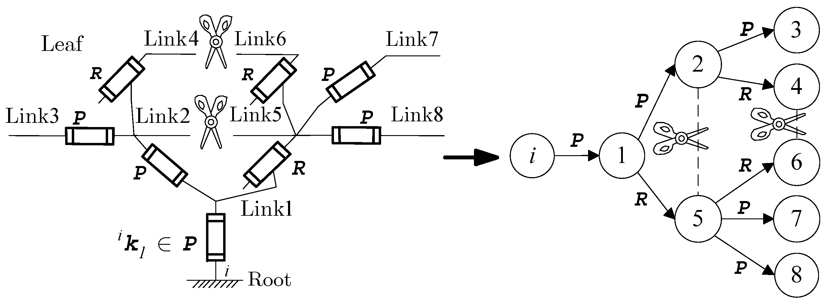
Figure 2.
Schematic and natural reference system of the 6-DOF manipulator.
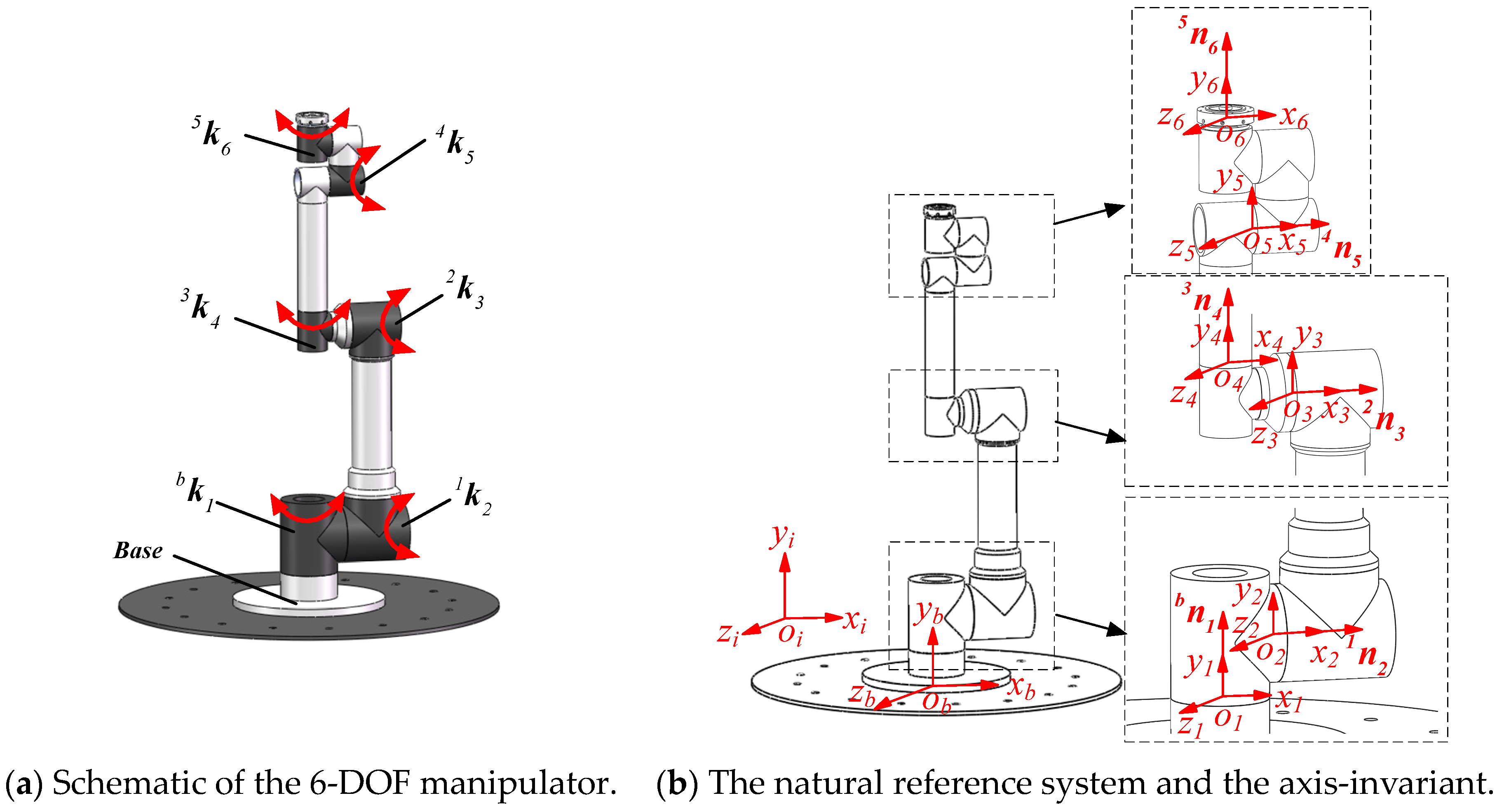
Figure 3.
Schematics of the axis-invariants () of the revolute joint and the prismatic joint.

Figure 4.
Schematic of the spanning tree chain corresponding to single-loop closed chain.

Figure 5.
3D motion screw.
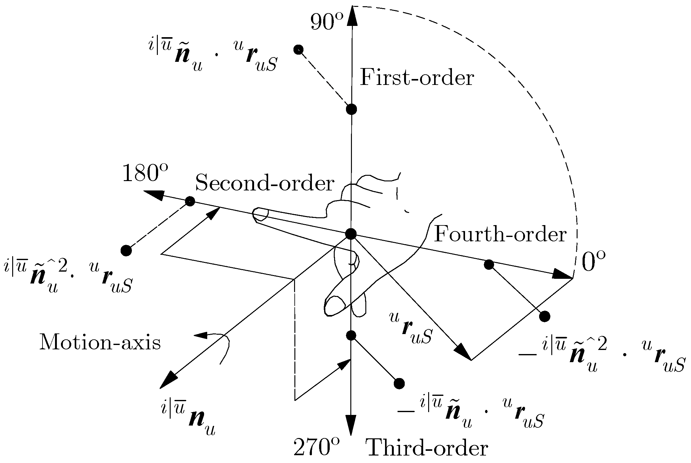
Figure 6.
3D force screw.

Figure 7.
Coulomb friction and viscous friction for the revolute joint and prismatic joint.

Figure 8.
The geometric models of the revolute joint and the prismatic joint.

Figure 9.
The physical diagram of the 6-DOF manipulator.

Figure 10.
The variation in the friction torque of joint 4 with respect to the braking speed.

Figure 11.
Schematic of the Coulomb–viscous friction model and the Stribeck friction model.
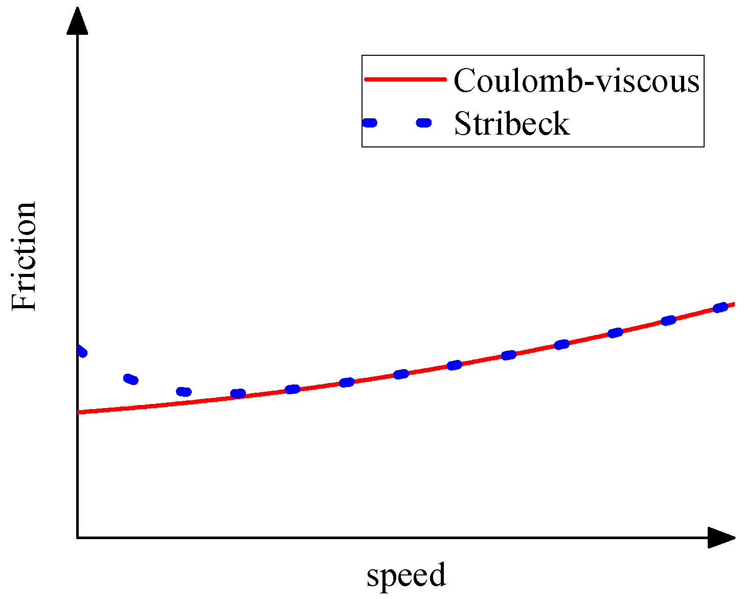
Figure 12.
Five-axis tree-chain mechanism and corresponding topological analysis.

Figure 13.
Constraint resultant torques of joints 1, 2, and 4.

Figure 14.
Constraint resultant forces of joints 1, 2, and 4.

Figure 15.
Driving torque of joints 1, 2, and 4.
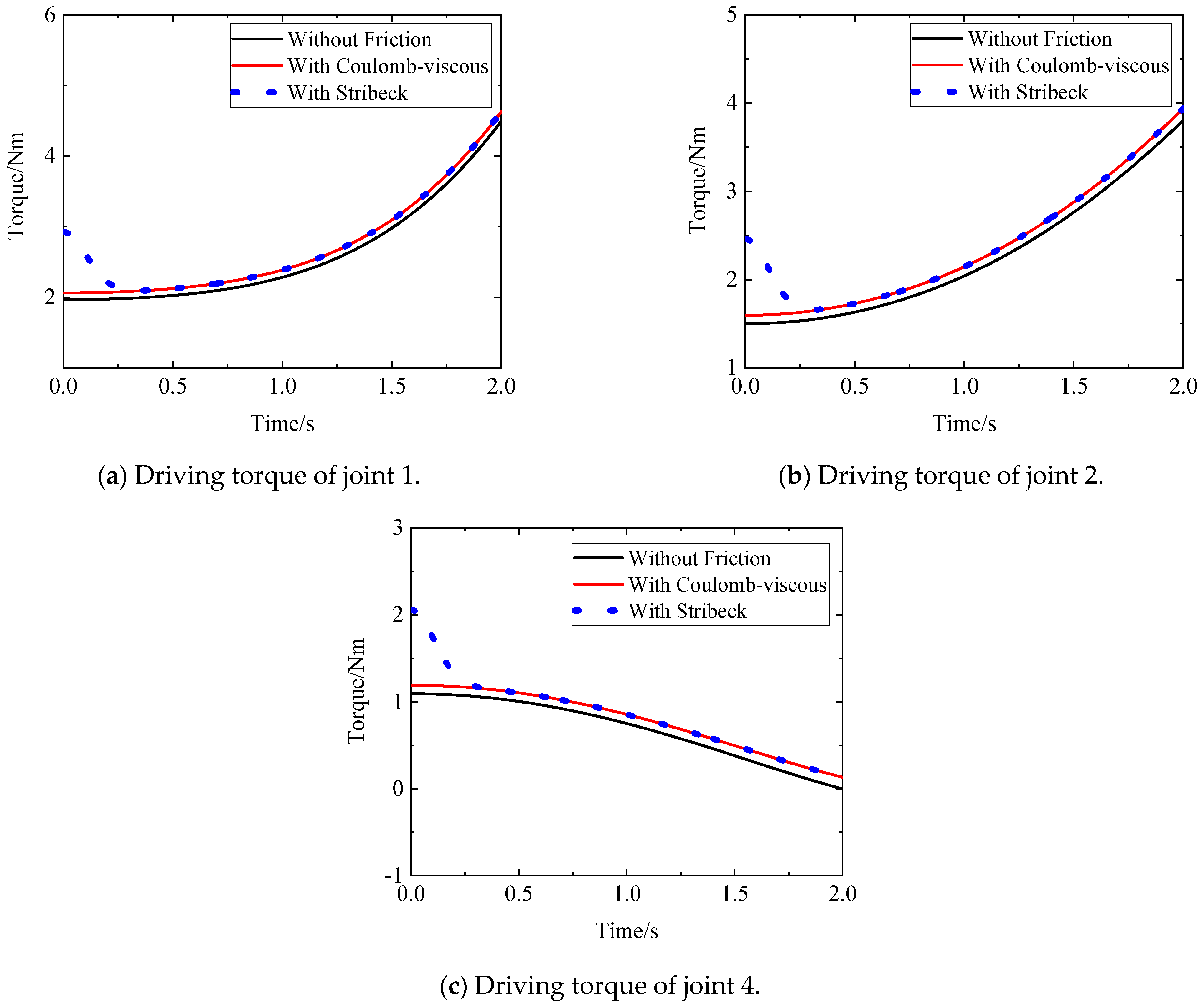
Figure 16.
Three-loop closed-chain mechanism and corresponding topological analysis.

Figure 17.
Rotation angles of six passive joints.

Figure 18.
Constraint forces of three closed-loop joints.

Figure 19.
Constraint force of the active joint.

Table 1.
Symbol descriptions.
| Type | Symbol | Description | Symbol | Description |
|---|---|---|---|---|
| Topology | Closed subtree of link u | Kinematic chain from i to l | ||
| Structure | Axis-invariant | Vector from to | ||
| Kinematic | Angular position along | Vector form of | ||
| Linear position along | Vector form of | |||
| Absolute angular velocity vector of joint l | Absolute angular acceleration vector of joint l | |||
| Absolute translational velocity vector of joint l | Absolute translational acceleration vector of joint l | |||
| Rotation matrix from to | 3D identity matrix | |||
| Dynamic | Mass of link k | Inertia tensor of link k | ||
| Inertial force matrix of revolute joint u | Bias force vector of revolute joint u | |||
| Inertial force matrix of prismatic joint u | Bias force vector of prismatic joint u | |||
| Resultant torque on axis except gravity | Resultant force on axis except gravity | |||
| Driving torque on axis | Driving force on axis | |||
| Mathematical operation | Exponent operator | Transpose operator | ||
| Derivative operator | Second derivative operator | |||
| Cross-product operator | Projection operator |
Table 2.
Initial parameters.
| Parameter | Symbol | Value |
|---|---|---|
| Axis-invariant | , , , , | [0 0 1]T |
| Initial linear position | ; ; | [−0.4 0 0]T; [0.6 1.0392 0]T; |
| ; | [−0.2 0 0]T; [0.6 −1.0392 0]T | |
| Central position of link mass | ;; | [−0.2 0 0]T; [0.3 0.5196 0]T; |
| ;; | [0.3 −0.5196 0]T; [0.3 −0.5196 0]T; | |
| [0.3 0.5196 0]T | ||
| Link mass | 1 kg | |
| , | 3 kg | |
| , | 2 kg | |
| Link MOI | diag(0.002, 0.01, 0.01) kg·m2 | |
| , | diag(0.008, 0.06, 0.06) kg·m2 | |
| , | diag(0.005, 0.04, 0.04) kg·m2 | |
| Gravitational acceleration | [0 0 −9.8]T m/s2 | |
| Driving angular acceleration | , , , , | 0.2 rad/s2 |
| Coulomb friction coefficient | , , , , | 0.005 |
| Viscous friction coefficient | , , , , | 0.01 |
| Static friction coefficient | , , , , | 0.05 |
| Stribeck velocity | , , , , | 0.03 |
Table 3.
Initial parameters.
| Parameter | Symbol | Value |
|---|---|---|
| Axis-invariant | , , , , , , | [0 0 1]T |
| Initial linear position | ; | [0.0737 −0.0676 0]T; [−0.0451 −0.0217 0]T; |
| ; ; | [−0.0375 0.0249 0]T; [0.0368 −0.0338 0]T; | |
| ; ; | [−0.0457 −0.0306 0]T; [−0.0079 −0.0544 0]T; | |
| ; ; | [0.049 −0.01 0]T; [−0.049 0.01 0]T; | |
| [−0.0069 −0.0445 0]T; | ||
| Central position of the link mass | ; ; | [0.0369 −0.0338 0]T; [−0.0451 −0.0217 0]T; |
| ; ; | [−0.0187 0.0124 0]T; [−0.0229 −0.0153 0]T; | |
| ; ; | [−0.0039 −0.0272 0]T; [0 0 0]T; | |
| [−0.0034 −0.0222 0]T | ||
| Link mass | , , | 2 kg |
| , | 1 kg | |
| , | 1.2 kg | |
| Link MOI | , , | diag(0.005, 0.04, 0.04) kg·m2 |
| , | diag(0.002, 0.01, 0.01) kg·m2 | |
| , | diag(0.003, 0.02, 0.02) kg·m2 | |
| Gravitational acceleration | [0 −9.8 0]T m/s2 | |
| Driving angular velocity | 0.1 rad/s | |
| Coulomb friction coefficient | 0.05 | |
| Viscous friction coefficient | 0.01 | |
| Static friction coefficient | 0.2 | |
| Stribeck velocity | 0.1 |
Disclaimer/Publisher’s Note: The statements, opinions and data contained in all publications are solely those of the individual author(s) and contributor(s) and not of MDPI and/or the editor(s). MDPI and/or the editor(s) disclaim responsibility for any injury to people or property resulting from any ideas, methods, instructions or products referred to in the content. |
© 2024 by the authors. Licensee MDPI, Basel, Switzerland. This article is an open access article distributed under the terms and conditions of the Creative Commons Attribution (CC BY) license (https://creativecommons.org/licenses/by/4.0/).
Share and Cite
MDPI and ACS Style
Guo, Z.; Ju, H.; Wang, K. A Novel Explicit Canonical Dynamic Modeling Method for Multi-Rigid-Body Mechanisms Considering Joint Friction. Aerospace 2024, 11, 368. https://doi.org/10.3390/aerospace11050368
AMA Style
Guo Z, Ju H, Wang K. A Novel Explicit Canonical Dynamic Modeling Method for Multi-Rigid-Body Mechanisms Considering Joint Friction. Aerospace. 2024; 11(5):368. https://doi.org/10.3390/aerospace11050368
Chicago/Turabian StyleGuo, Zhenhao, Hehua Ju, and Kaimeng Wang. 2024. "A Novel Explicit Canonical Dynamic Modeling Method for Multi-Rigid-Body Mechanisms Considering Joint Friction" Aerospace 11, no. 5: 368. https://doi.org/10.3390/aerospace11050368
Note that from the first issue of 2016, this journal uses article numbers instead of page numbers. See further details here.