Ternary Hybrid Nanofluid Flow Containing Gyrotactic Microorganisms over Three Different Geometries with Cattaneo–Christov Model

Abstract

The movement of microorganism cells in fluid influences various biotic processes, including septicity and marine life ecology. Many organic and medicinal applications need to look into the insight of mechanism in nanofluids containing a microbial suspension. The current paper concerns the bioconvection of a ternary hybrid nanofluid (Al₂O₃-Cu-CNT/water) flow containing motile gyrotactic microorganisms toward three different geometries (a flat plate, a wedge, and a cone) in the occurrence of natural convection, radiation, and heat source/sink. The Cattaneo–Christov theory is employed to develop the model. The equations are solved by using the “bvp4c function in MATLAB”. The influence of the crucial significant factors on the motile microorganisms’ density, velocity, temperature, nanoparticles’ concentration, microbe density gradient, and transmission rates of heat and mass is discussed. The results depict that the heat transmission rate is highest for the flow toward the cone, whereas the mass transmission rate and microbe density gradient are highest for the flow toward the wedge. In addition, the higher estimates of the thermal relaxation parameter corresponding to the Cattaneo–Christov theory act to enhance the rate of heat transmission. The results of the current study will be useful to many microbial-enhanced oil recovery systems, carriage processes, architectural design systems, medicinal fields that utilize nanofluids, and so on.

1. Introduction

The importance of NF and HNF flow over a wedge, a cone, and a flat plate is due to their vast applications. These applications are seen in, but are not restricted to, fiber technology, the design of vessels for nuclear waste retention, steam generators, spacecraft design, and solar power collectors. Initially, for the aforementioned applications, manufacturers utilized lubricants, air, and water to accomplish heat transmission (HT). However, such natural materials do not fulfill the standards at the industrial scale. Many working fluids have poor thermal conductivity (TC), which is considered a hurdle in HT, and it slows down the working of thermal flow models. In the present world, the production of several gadgets and apparatuses utilized in industrial and technical arenas has evolved significantly. For instance, in various devices, temperature rises over time, owing to electrical resistance. The heat-transport capacity of such devices is diminished due to electric resistance, resulting in a technical defect. To lessen the possibility of a technical malfunction, many devices and components must be heat-intolerant. Therefore, these applications require a coolant that has superior TC and heat transfer qualities. Previous research (Choi [1]) has demonstrated that dispersing nanoparticles (NPs) in a base fluid dramatically changes the characteristics and heat transfer qualities of a convectional base fluid (BF). Furthermore, if necessary, the characteristics of nanofluids (NFs) can be tailored to a specific purpose. The main limitation with an NF containing a single type of NPs is that the NPs have better thermal linkages or good rheological features, but not both. The properties of NFs may be enhanced by altering the nanoparticles volume fraction (NVF); however, this has a restriction because of the difficulties arising owing to viscosity escalation. To erase the limitation of NFs, researchers studied hybrid nanofluids (HNFs) that aim to elevate the properties of nanoparticles of different materials. Early HNFs studies employed NFs with two different particles; however, in the last three years, a distinct research trend has evolved that consists of mixing several NPs to generate an ideal nanofluid: three NPs in a working fluid. Such NFs are mentioned as “ternary nanofluids”, “ternary hybrid nanofluids” (THNF), or “trihybrid nanofluids.” The authors of the present study have studied the comparative behavior of bioconvective THNF flow over three different geometries (a flat plate, a wedge, and a cone). The main aim of the authors is to investigate the HT rate of THNF (Al₂O₃-Cu-CNT/water) over the surface of three different geometries (a flat plate, a wedge, and a cone).

In their review article, Sahoo [2] and Adun et al. [3] emphasized the shapes of NPs, the material of NPs, the size of NPs, and the proportion of NPs in optimizing the properties of THNF. Furthermore, selecting the appropriate NPs mixture, as well as optimal NPs mixing and stability, are critical variables that may influence THNF development, notably for HT applications (Xuan et al. [4]). The invention of THNFs and the experimental validation of correlations (Sahoo and Kumar [5] and Sahoo [6]) have paved the way for researchers working in numerical flow analysis to investigate the possibility of THNFs as a viable coolant in industrial HT applications. Animasaun et al. [7] expounded the significance of convective heating on the transport of THNF over a horizontal surface stretching with a linear rate. They investigated the flow with water as a BF and aluminum oxide, aluminum, and silver NPs, all with different shapes. They concluded that convective heating could be utilized for achieving a high HT rate. Alanazi et al. [8] recently studied the dynamics of ternary-hybrid nanofluid subject to magnetic flux density and heat source or sink on a convectively heated surface. They deduced that increasing thermo-migration of NPs causes HT to reduce. Raju et al. [9] explicated the nonlinear movements of axisymmetric ternary hybrid nanofluids in a thermally radiated expanding or contracting permeable Darcy Walls with different shapes and densities by using simple linear regression. Ramzan et al. [10] expounded on the influence of ion slip and Hall current on kerosene-based THNF flow towards a surface rotating about an axis with silver, copper, and graphene oxide NPs.

Improvement of thermal control is a concern of manufacturers of the electrical division, thermal systems, power sector, and medicinal bids. To study the HT rate in any medium, it is of utmost importance to see the regulations of HT in that particular medium. For a long period, HT was analyzed with the Fourier law [11], which says that HT occurs at an infinite speed. Later, Cattaneo [12] modified the law of Fourier by generalizing it and stating that HT occurs at a restricted speed in any medium. He incorporated a time relaxation factor to generalize the Fourier model, and it reduced the nature of the parabolic thermal equation to a hyperbolic equation. Christov [13] achieved the material invariant form of Cattaneo’s law through the Oldroyd derivative. After the successful formulation by Cattaneo and Christov, the model came to be known as the Cattaneo–Christov heat flux model (CCHM). Numerous researchers have calculated the HT rate of different flows with a time lag factor using CCHM. Venkateswarlu et al. [14] expounded on the significance of CCHM in nanofluid flow past a surface with a linear stretching rate. They discussed the nanofluid flow with BF as water, discussed the flow pattern, and presented a comparison of MoS₂/water and MgO/water nanofluid. Rawat and Kumar [15] analyzed Cu-water NF flow over a stretching surface with CCHM and inferred that time lag presence reduces the HT rate. Ramzan et al. [16] expounded on the flow behavior of dusty micropolar NF flow over a sheet with CCHM. Lv et al. [17] studied the significance of CCHM in Reiner–Rivlin NF flow over a disk rotating about an axis with bioconvection phenomena. Abderrahmane et al. [18] elucidated the impact of MHD Hybrid Nanofluid Mixed Convection Heat Transfer and Entropy Generation in a 3-D Triangular Porous Cavity with Zigzag Wall and Rotating Cylinder.

Another intriguing study field is the bioconvection phenomenon, which covers a range of applications in the real world. The directed movement of diverse microorganisms functions as the base for many bioconvection models. Different species are distinguished by the direction in which these microorganisms swim. Gyrotactic microbes (GM) are the ones that travel upwards against gravity in stagnant water, resulting in the higher section of the fluid being denser than the lower. When the higher portion gets too dense, owing to microbe accumulation, it becomes unstable, and microbes fall, causing bioconvection. This bioconvection pattern is maintained by returning swimming microorganisms. Applications of this phenomenon include biological tissues, biofuels, biotechnology, microsystems, transportation processes, enzyme biosensors, microbial-enhanced oil recovery, and so on. Furthermore, bioconvective nanofluid has vast applications, including the development of nanoparticle processing, architectural design, nanoparticle stability, polymer coating, automobile coolants, and sterilizing applications in thermal sciences, among others. The novel idea of nanofluid with different nanoparticles are presented in [19,20,21]. Shi et al. [22] explicated the idea of a magnetic bioconvective stream of a Cross nanoliquid over a stretched sheet. They determined that the growing Lewis number causes the density of gyrotactic microorganisms (GM) to fall. Al Khaled and Khan et al. [23] expounded on the thermal properties of a Casson nanoliquid flow containing GM over a surface in motion. Bhatti et al. [24] explicated the applications of GM in blood-based non-Newtonian nanoliquid flow through a narrow artery. They utilized the Sutterby fluid model to study blood flow. Kairi et al. [25] expounded on the significance of the suspension of GM in a Casson nanoliquid flow past an inclined, stretched sheet with Marangoni convection. Ali et al. [26] explicated the magnetic Cross nanomaterial flow over an extending horizontal plate and horizontal cylinder and studied the significance of GM and CCHM in their flow model.

Of late, several researchers have published papers on the flow of NFs or HNFs over a cone, a wedge, and a flat plate (Mishra and Kumar [27] and Yaseen et al. [28], Mahanthesh and Mackolil [29], and Gumber et al. [30]). In this research communication, authors have modeled and investigated the bioconvective THNF flow (Al₂O₃-Cu-CNT/water flow) over three different geometries (a flat plate, a wedge, and a cone) with motile gyrotactic microorganisms (GM). Moreover, the significance of CCHM, heat generation/absorption, natural convection, and thermal radiation are also studied. Some past research (see, for instance, Rawat et al. [31], Sandeep and Reddy [32], and Reddy et al. [33]) has conducted such comparative studies. However, until now, no author(s) have attempted or published a study, which shows the comparative behavior of bioconvective THNF (Al₂O₃-Cu-CNT/water) flow over three different geometries (a flat plate, a wedge, and a cone). The results of the current study will be useful to many microbial-enhanced oil recovery systems, carriage processes, architectural design systems, medicinal fields that utilize nanofluids, and so on. The novelty and aim of this research communication and the aspects this paper attempts to explore are as mentioned in the following points:

• The mathematical flow model of THNF (Al₂O₃-Cu-CNT/water) over three different geometries (a flat plate, a wedge, and a cone).
• The application of CCHM in the THNF flow.
• The significance of motile GM in THNF (Al₂O₃-Cu-CNT/water).
• Investigating the HT rate of THNF flow over three different geometries (a flat plate, a wedge, and a cone) and finding the condition/geometries under present modeling for which THNF has the maximum HT rate.
• Comparison of the HT rate of THNF flow with the HT rate of HNF and NF in the case of all three geometries.

2. Flow Model and Governing Equations

2.1. Flow Assumptions and Mathematical Model

This research communication explores the flow of THNF (Al₂O₃-Cu-CNT/water) toward three different geometries (a cone, a wedge, and a flat plate) containing motile GM. This section of the paper deals with the modeling of the flow of THNF in the boundary layer region (BLR) and the assumptions of the model. To study the THNF flow, the surface of a cone, wedge, and flat plate are assumed coincidental to the x-axis, and the y-axis is normal to it (refer to Figure 1). The flow is instigated by the manifestation of the convection effect. The half angle of the wedge and cone are denoted by α, and the radius of the cone is denoted by r. To overview the influence of the presence of time lag in the heat transfer (HT) and mass transfer (MT) rate, the authors modeled the flow with the Cattaneo–Christov theory. Furthermore, heat source/sink, thermal radiation, and injection/suction effects are also deliberated together to study the flow of THNF in the present problem. In the last term on the right hand side in the energy equation (Equation (3)), $q_r$ denotes the thermal radiative heat flux, and it is defined later, after governing equations.

Based on the assumptions and aforesaid discussion, the bioconvective flow of THNF (Al₂O₃-Cu-CNT/water) toward three different geometries (a flat plate, a wedge, and a cone) is represented by the following PDEs [34,35]:

Continuity equation:

$$\frac{\partial (r^{n}u)}{\partial x}+\frac{\partial (r^{n}v)}{\partial y}=0$$

(1)

Since the thermal BLR thickness is very minuscule, the $r=xsin\left(\alpha \right)$.

Momentum equations:

$$u\frac{\partial u}{\partial x}+v\frac{\partial u}{\partial y}={\nu }_{thnf}\left(\frac{{\partial }^{2}u}{\partial y^2}\right)+\frac{{(\rho \beta )}_{thnf}}{{\rho }_{thnf}}g\left(T-T_{\infty }\right)\cos \alpha$$

(2)

Energy equation:

$$\begin{array}{r}{\left(\rho C_p\right)}_{thnf}\left\{u\frac{\partial T}{\partial x}+v\frac{\partial T}{\partial y}+{\tau }_t\left(\begin{array}{l}{u}^2\frac{{\partial }^{2}T}{\partial x^2}+\left(u\frac{\partial u}{\partial x}+v\frac{\partial u}{\partial y}\right)\frac{\partial T}{\partial x}+\left(u\frac{\partial v}{\partial x}+v\frac{\partial v}{\partial y}\right)\frac{\partial T}{\partial y}\\ +2uv\frac{{\partial }^{2}T}{\partial x\partial y}+v^2\frac{{\partial }^{2}T}{\partial y^2}-\frac{Q_o}{{(p{C}_p)}_{thnf}}\left(u\frac{\partial T}{\partial x}+v\frac{\partial T}{\partial y}\right)\end{array}\right)\right\}\\ =k_{thnf}\frac{{\partial }^{2}T}{\partial y^2}+Q_0\left(T-T_{\infty }\right)-\frac{\partial q_r}{\partial y}\end{array}$$

(3)

Concentration equation:

$$u\frac{\partial C}{\partial x} + v\frac{\partial C}{\partial y} +{\tau }_c\left[u^2\frac{{\partial }^{2}C}{\partial x^2}+\left(u\frac{\partial u}{\partial x}+v\frac{\partial u}{\partial y}\right)\frac{\partial C}{\partial x}+\left(u\frac{\partial v}{\partial x}+v\frac{\partial v}{\partial y}\right)\frac{\partial C}{\partial y}+2uv\frac{{\partial }^{2}C}{\partial x\partial y}+v^2\frac{{\partial }^{2}C}{\partial y^2}\right]=D_n\frac{{\partial }^{2}C}{\partial y^2}$$

(4)

Microorganisms’ equation:

$$u\frac{\partial N}{\partial x}+v\frac{\partial N}{\partial y}+\left(\frac{b{W}_c}{C_w-C_{\infty }}\right)\left(\frac{\partial }{\partial y}\left(N\frac{\partial C}{\partial y}\right)\right)=D_m\frac{{\partial }^{2}N}{\partial y^2}$$

(5)

where “$\left(u,v\right)$ are the velocity components along $\left(x,y\right)$ directions”, respectively. In addition, the variables used in Equations (1)–(6) have the following meaning: “T—temperature”, “C—concentration”, “N—motile microorganisms concentration”, “Q₀—heat source/sink coefficient”, “b—chemotaxis constant”, “W_c—swimming cells speed”, “${\tau }_t$—thermal relaxation time”, “${\tau }_c$—solutal relaxation time”. Furthermore, “k—thermal conductivity, $\mu$—dynamic viscosity, $\nu$—kinematic viscosity, $C_p$—heat capacity, $\rho$—density, $\sigma$—electrical conductivity, D_n—Brownian diffusion coefficient, and D_m—microorganisms diffusion”. Moreover, subscript w—wall condition, $\infty$—free stream condition, thnf—ternary hybrid nanofluid, nf—nanofluid, and bf—fluid.

Furthermore, at the surface, suction/injection is applied with v_w as velocity of mass transfer, and surface is moving with initial velocity, as $u_w={\nu }_{f}x/l^2$. The temperature at the surface $T_w$ is taken as a variable $T_w=T_{\infty }+a{x}^s$, where $T_{\infty }$ is the free stream temperature of THNF, and s is the parameter related to surface temperature. In addition, $C_w$ and $N_w$ are concentrations of NPs and GM at the surface, whereas $C_{\infty }$ and $N_{\infty }$ are concentrations of NPs and GM at the free stream.

The Boundary Conditions (BCs) are:

$$\begin{array}{l}u=u_w=\frac{{\nu }_f x}{l^2}, v=v_w, T=T_w=T_{\infty }+a{x}^s, C=C_w, N=N_w \mathrm{at} y = 0\\ u\to 0, T\to T_{\infty }, \mathrm{C}\to C_{\infty }, N\to N_{\infty } \mathrm{as} y\to \infty \end{array}\}$$

(6)

The Rosseland theory is used to approximate the thermal radiative heat flux $q_r$, and it is demarcated as follows [15]:

$$q_r=-\frac{4{\sigma }^{*}}{3k^{*}}\frac{\partial T^4}{\partial y}$$

(7)

where “k^* is the mean absorption coefficient”, and “σ^* is the Stefan-Boltzmann constant”. In Equation (7), the value of $q_r$ is estimated by assuming $T^4\cong 4T_{\infty }{}^{3}T-3T_{\infty }{}^4$ with the help of expansion via Taylor’s series. This assumption is valid for flow that has minuscule temperature differences in the layers. To arrive at such an assumption, higher-order terms are neglected in Taylor’s series expansion about $T_{\infty }$. The energy equation (Equation (3)) is further solved with the help of Equation (7) and the aforementioned assumption of $T^4$.

The flow of THNF (Al₂O₃-Cu-CNT/water) toward three different geometries (a cone, a wedge, and a flat plate) is characterized by the following conditions [32,35]:

(a)

THNF flow toward cone: n = 1 and α ≠ 0.

(b)

THNF flow toward wedge: n = 0 and α ≠ 0.

(c)

THNF flow toward flat plate: n = 0 and α ≠ 0.

2.2. Properties of Ternary Hybrid Nanofluid

The current subsection refers to the modeling and investigation of THNF. The characteristics of THNF are subjected to the base fluid (water), NPs, and the NVF of Al₂O₃, Cu, and CNT NPs, as presented in

Table 1. Thermo-physical properties of water, Al₂O₃, Cu, and CNT nanoparticles [15,36].

	ρ (kg/m3)	Cp (J/kgK)	k (W/mK)	β (K−1)	Shape	Sphericity
Water	997.1	4179	0.613	21
Al2O3	3970	765	40	0.85	Spherical	ψ = 1
Cu	8933	385	401	1.67	Platelet	ψ = 0.612
CNT	2600	425	6600	1.6 × 10−6	Cylindrical	ψ = 0.52

[15,36]. Moreover, the authors investigated the effect of differently shaped nanoparticles (CNT—cylindrical, Cu—platelet, and Al₂O₃—spherical) on the thermal behavior of the THNF in this study.

Table 2. Thermophysical properties of ternary hybrid nanofluid [36,37].

Density	${\rho }_{thnf}=\left(1-{\varphi }_1-{\varphi }_2-{\varphi }_3\right){\rho }_{bf}+{\varphi }_1{\rho }_{sp1}+{\varphi }_2{\rho }_{sp2}+{\varphi }_3{\rho }_{sp3}$
Heat capacitance	${\left(\rho C_p\right)}_{thnf}=\left(1-{\varphi }_1-{\varphi }_2-{\varphi }_3\right){\left(\rho C_p\right)}_{bf}+{\varphi }_1{\left(\rho C_p\right)}_{sp1}+{\varphi }_2{\left(\rho C_p\right)}_{sp2}+{\varphi }_3{\left(\rho C_p\right)}_{sp3},$
Modified Maxwell model:		$\frac{k_{n{f}_i}}{k_{bf}}=\frac{k_i+\left(n-1\right)k_{bf}+\left(n-1\right){\varphi }_i\left(k_i-k_{bf}\right)}{k_i+\left(n-1\right)k_{bf}-{\varphi }_i\left(k_i-k_{bf}\right)}$ where, $n=\left(\frac{3}{\psi }\right)$ is shape factor.
Nanoparticle—1	(Spherical)	$\Rightarrow \{\begin{array}{c}\frac{{\mu }_{nf1}}{{\mu }_{bf}}=1+2.5{\varphi }_1+6.2{\varphi }_1^2\\ \frac{k_{nf1}}{k_{bf}}=\frac{k_1+2k_{bf}+2{\varphi }_1\left(k_1-k_{bf}\right)}{k_1+2k_{bf}-{\varphi }_1\left(k_1-k_{bf}\right)}\end{array}$
Nanoparticle—2	(Platelet)	$\Rightarrow \{\begin{array}{c}\frac{{\mu }_{nf2}}{{\mu }_{bf}}=1+13.5{\varphi }_2+904.4{\varphi }_2^2\\ \frac{k_{nf2}}{k_{bf}}=\frac{k_2+3.9k_{bf}+3.9{\varphi }_2\left(k_2-k_{bf}\right)}{k_2+3.9k_{bf}-{\varphi }_2\left(k_2-k_{bf}\right)}\end{array}$
Nanoparticle—3	(Cylindrical)	$\Rightarrow \{\begin{array}{c}\frac{{\mu }_{nf3}}{{\mu }_{bf}}=1+37.1{\varphi }_3+612.6{\varphi }_3^2\\ \frac{k_{nf3}}{k_{bf}}=\frac{k_3+4.7k_{bf}+4.7{\varphi }_3\left(k_3-k_{bf}\right)}{k_3+4.7k_{bf}-{\varphi }_3\left(k_3-k_{bf}\right)}\end{array}$
Viscosity	${\mu }_{thnf}=\frac{{\mu }_{nf1}{\varphi }_1+{\mu }_{nf2}{\varphi }_2+{\mu }_{nf3}{\varphi }_3}{{\varphi }_{thnf}}$
Thermal conductivity	$k_{thnf}=\frac{k_{nf1}{\varphi }_1+k_{nf2}{\varphi }_2+k_{nf3}{\varphi }_3}{{\varphi }_{thnf}}$	Where ${\varphi }_{thnf}={\varphi }_1+{\varphi }_2+{\varphi }_3$

lists the models used to develop thermophysical correlations of the properties of THNF [36,37]. These correlations are valid and provide precise results when the NVF is taken between the range of 0.01 to 0.1 and temperature range is between 35 °C to 50 °C. In this paper, NVF of Al₂O₃, Cu, and CNT NPs is denoted by ${\phi }_1$, ${\phi }_2$, and ${\phi }_3$. Furthermore, the following subscripts are used for: sp₁—Al₂O₃, sp₂—Cu, and sp₃—CNT NPs.

2.3. Conversion of the Model Equations with Similarity Transformation

The flow governing PDEs (Equations (1)–(6)) are first modified using the similarity transformation [32,38]:

$$\eta =\frac{y}{l}, u=\frac{{\nu }_{f}x}{l^2}{f}^{\prime }\left(\eta \right), v=- \left(n+1\right){\nu }_f\frac{f\left(\eta \right)}{l}, \theta \left(\eta \right)=\frac{T-T_{\infty }}{T_w-T_{\infty }}, \varphi \left(\eta \right)=\frac{C-C_{\infty }}{C_w-C_{\infty }}, \zeta =\frac{N-N_{\infty }}{N_w-N_{\infty }}$$

(8)

The continuity equation (Equation (1)) is identically satisfied, and the same can be verified by utilizing the similarity transformations from Equation (7) in the continuity equation (Equation (1)). The reduced form of Equations (2)–(5) and BCs (Equation (6)) after using similarity transformations are as follows:

Reduced Momentum equation:

$${f^{\prime }}^2- \left(n+1\right){ff}^{″}=\frac{{∍}_1}{{∍}_2}{f}^{‴}+\frac{{∍}_3}{{∍}_2}\lambda \theta \cos \alpha$$

(9)

Reduced Energy equation:

$$s{f}^{\prime }\theta - \left(n+1\right)f{\theta }^{\prime }+{\gamma }_t\left[\begin{array}{l}s\left(s-1\right){f^{\prime }}^2\theta +s\left(\theta {f^{\prime }}^2- \left(n+1\right)\theta f{f}^{″}\right)\\ +{\left(n+1\right)}^2{\theta }^{\prime }f{f}^{\prime }-2\left(n+1\right)sf{f}^{\prime }{\theta }^{\prime }\\ + {\left(n+1\right)}^2{f}^2{\theta }^{″}-\frac{Q}{{∍}_4}\left(s\theta f^{\prime }- \left(n+1\right)f{\theta }^{\prime }\right)\end{array}\right]=\frac{1}{{∍}_4\mathrm{Pr}}\left({∍}_5+\frac{4}{3}{R}_d\right){\theta }^{″}+\frac{Q}{{∍}_4}\theta$$

(10)

Reduced Concentration equation:

$${\varphi }^{″}+Le\left(n+1\right)f{\varphi }^{\prime } -Le{\left(n+1\right)}^2{\gamma }_c\left\{f{f}^{\prime }{\varphi }^{\prime }+f^2{\varphi }^{″}\right\}=0$$

(11)

Reduced Microorganisms’ equation:

$${\zeta }^{″}-Pe\left({\zeta }^{\prime }{\varphi }^{\prime }+\left(\varpi +\zeta \right){\varphi }^{″}\right)+\left(n+1\right)Lbf{\zeta }^{\prime }=0$$

(12)

Reduced BCs:

$$\begin{array}{l}{f}^{\prime }\left(0\right)=1, f\left(0\right)=\frac{Su}{\left(n+1\right)}, \theta \left(0\right)=1, \varphi \left(0\right)=1, \zeta \left(0\right)=1 \mathrm{at} \eta = 0\\ f^{\prime }\left(0\right)=0, \theta \left(0\right)=0, \varphi \left(0\right)=0, \zeta \left(0\right)=0 \mathrm{as} \eta \to \infty \end{array}\}$$

(13)

In the aforementioned Equations (9)–(12) and BCs (Equation (13)), the nondimensional parameters are encountered, and they are named and defined as follows:

“$\lambda \left(=G{r}_x/R{e}_x{}^2\right)$—Natural convection parameter, where $G{r}_x\left(=g{\beta }_f\left(T_w-T_{\infty }\right)l^4/x{\nu }_f{}^2\right)$—Local Grashof number, $R{e}_x=\left(u_{w}x/v_f\right)$—Local Reynolds number. Furthermore, $Pr(={(\rho c_p)}_f{\nu }_f/k_f)$ —Prandtl number, $R_d=\left(4{\sigma }^{*}{T}_{\infty }^3/k_f{k}^{*}\right)$—Thermal radiation parameter, $Q\left(=Q_0{l}^2/{(\rho C_p)}_f{\nu }_f \right)$—Heat source/sink parameter, and ${\gamma }_t=\left({\tau }_t{\nu }_f/l^2\right)$—Thermal relaxation parameter. In addition, $Le\left(=v_f/D_n\right)$—Lewis number, $Lb\left(=v_f/D_m\right)$—bioconvection Lewis number, $Pe\left(=b{W}_c/D_m\right)$—bioconvection Peclet number, $\varpi \left(=N_2/\left(N_1-N_2\right)\right)$—bioconvection constant, ${\gamma }_c=\left({\tau }_c{\nu }_f/l^2\right)$—Solutal relaxation parameter, and $Su=\left(-v_{w}l/v_f\right)$—Suction/Injection parameter. Furthermore, ${∍}_1={\mu }_{thnf}/{\mu }_f, {∍}_2={\rho }_{thnf}/{\rho }_f, {∍}_3={(\rho \beta )}_{thnf}/{(\rho \beta )}_f, {∍}_4={(\rho C_p)}_{thnf}/{(\rho C_p)}_f, {∍}_5=k_{thnf}/k_f$ are constants based on THNF correlations and properties (see Table 2)”.

To have similar solutions of the Equations (9)–(12) with the BCs (Equation (13)), the term of x must vanish from these equations. It is noticed that the natural convection parameter $\lambda \left(=G{r}_x/R{e}_x{}^2\right)$ appearing in Equation (9) when computed in the simplified form will be written as $\lambda =g{\beta }_f\left(T_w-T_{\infty }\right)l^4/{\nu }_f^{2}x$. Further, the BCs (Equation (6)) imply that surface temperature is in a variable form, as $T_w=T_{\infty }+a{x}^s$. So, further simplification will lead to the value of the natural convection parameter as $\lambda =g{\beta }_{f}a{x}^{s-1}{l}^4/{\nu }_f^2$. Therefore, a similar solution will exist only when $s=1$ because the term of x will vanish. For a similar solution to exist and for the computations of the results of this study, the value of the parameter related to surface temperature is strictly restricted to $s=1$.

3. Engineering Parameters

The analysis of the concerned and related engineering parameters is necessary while studying a flow model because it helps in applying the bids of the flow model in real-life applications. The “Nusselt number Nu” (representing heat transfer rate), “Sherwood number Sh” (representing mass transfer rate), and motile microorganism density gradient (Nm), at the surface of the flat plate, wedge, and cone, respectively, are [24,39]:

$$Nu=-\left({∍}_5+R_d\right){\theta }^{\prime }\left(0\right)$$

(14)

$$Sh=-{\phi }^{\prime }\left(0\right)$$

(15)

$$Nm=-{\zeta }^{\prime }\left(0\right)$$

(16)

4. Methodology of Numerical Approach

The current section demonstrates the approach taken to solve the model depicted by similarity equations (Equations (9)–(12)) and BCs (13). The transfigured equations are nonlinear and coupled. Deducing an analytical solution to such a system is not an easy task. Therefore, the authors attempted to solve the system (Equations (9)–(12)) and BCs (13) numerically. The numerical solution of the Equations is derived with the “bvp4c function (a built-in package in MATLAB)”. The “bvp4c function” uses a finite difference scheme together with a precision of fourth-order with the help of the “3-stage Lobatto IIIA formula”. The step-by-step working of bvp4c function is provided by Shampine et al. [40]. To derive the solution of the present problem, the Equations (9)–(12) are transformed into ODEs of first-order with the help of following transformation:

$${\Im }_{\left(1\right)}=f, {\Im }_{\left(2\right)}=f^{\prime }, {\Im }_{\left(3\right)}=f^{″}, {\Im }_{\left(4\right)}=\theta , {\Im }_{\left(5\right)}={\theta }^{\prime }, {\Im }_{\left(6\right)}=\phi , {\Im }_{\left(7\right)}={\phi }^{\prime },{\Im }_{\left(8\right)}=\zeta ,{\Im }_{\left(9\right)}={\zeta }^{\prime }$$

(17)

Utilizing the new variables, the following MATLAB syntax is used:

$$\begin{array}{l}\Im \Im 1=\frac{{∍}_2}{{∍}_1}\left({\Im }_{\left(2\right)}{}^2- \left(n+1\right){\Im }_{\left(1\right)}{\Im }_{\left(3\right)}-\frac{{∍}_3}{{∍}_2}\lambda {\Im }_{\left(4\right)}\cos \alpha \right);\\ \Im \Im 2=-\frac{\frac{Q}{{∍}_4}{\Im }_{\left(4\right)}-{\Im }_{\left(2\right)}{\Im }_{\left(4\right)}+ \left(n+1\right){\Im }_{\left(1\right)}{\Im }_{\left(5\right)}-\gamma \left[\begin{array}{l}{\Im }_{\left(4\right)}{\Im }_{\left(2\right)}{}^2- \left(n+1\right){\Im }_{\left(4\right)}{\Im }_{\left(1\right)}{\Im }_{\left(3\right)}+{\left(n+1\right)}^2{\Im }_{\left(5\right)}{\Im }_{\left(1\right)}{\Im }_{\left(2\right)}\\ -2\left(n+1\right){\Im }_{\left(1\right)}{\Im }_{\left(2\right)}{\Im }_{\left(5\right)}-\frac{Q}{{∍}_4}\left({\Im }_{\left(4\right)}{\Im }_{\left(2\right)}- \left(n+1\right){\Im }_{\left(1\right)}{\Im }_{\left(5\right)}\right)\end{array}\right]}{\frac{1}{{∍}_4\mathrm{Pr}}\left({∍}_5+\frac{4}{3}{R}_d-\gamma {\left(n+1\right)}^2{\Im }_{\left(1\right)}{}^2\right)};\\ \Im \Im 3=-\frac{Le\left(n+1\right){\Im }_{\left(1\right)}{\Im }_{\left(7\right)} -Le{\left(n+1\right)}^2{\gamma }_c{\Im }_{\left(1\right)}{\Im }_{\left(2\right)}{\Im }_{\left(7\right)}}{\left(1+Le{\left(n+1\right)}^2{\gamma }_c{\Im }_{\left(1\right)}{}^2\right)};\\ \Im \Im 4=Pe\left({\Im }_{\left(9\right)}{\Im }_{\left(7\right)}+\left(\varpi +{\Im }_{\left(8\right)}\right)\left(\Im \Im 3\right)\right)-\left(n+1\right)Lb{\Im }_{\left(1\right)}{\Im }_{\left(9\right)};\end{array}$$

(18)

The following MATLAB syntax is used for BCs at the surface and far-field:

$$\begin{array}{l}{\Im }_{\left(2\right)}\left(0\right)=1, {\Im }_{\left(1\right)}\left(0\right)=\frac{Su}{\left(n+1\right)}, {\Im }_{\left(4\right)}\left(0\right)=1, {\Im }_{\left(6\right)}\left(0\right)=1, {\Im }_{\left(8\right)}\left(0\right)=1 \mathrm{at} \eta = 0\\ {\Im }_{\left(2\right)}\left(\eta \right)=0, {\Im }_{\left(4\right)}\left(\eta \right)=0,{\Im }_{\left(6\right)}\left(\eta \right)=0, {\Im }_{\left(8\right)}\left(\eta \right)=0 \mathrm{as} \eta \to \infty \end{array}\}$$

(19)

In addition, the values of slopes not known are guessed to begin the process of solving the equations. The iteration process is repeated, and the solution is acknowledged only when BCs are met (see Figure 2). In this model, η_max was taken as 6, as the conditions at this point were satisfied asymptotically, and step size was taken as 0.01. To authenticate the results of the present model, a comparison is outlined with the published results of Vajravelu and Nayfeh [38] (see

Table 3. Comparison of values of $f^{″}\left(0\right) \mathrm{and}-{\theta }^{\prime }\left(0\right)$ with results of Vajravelu and Nayfeh [38] for the flow over cone when R_d = 0, ${\gamma }_t={\gamma }_c=0$, Su = 0; Le = Lb = Pe = $\varpi$ = 0.

Q	Pr	Gr	M	s	$${\mathit{f}}^{″}\left(0\right) (\mathbf{See} [38\left]\right)$$	$${\mathit{f}}^{″}\left(0\right) \left[\mathbf{Present}\right]$$	$$-{\mathit{\theta }}^{\prime }\left(0\right) (\mathbf{See} [38\left]\right)$$	$$-{\mathit{\theta }}^{\prime }\left(0\right) \left[\mathbf{Present}\right]$$
−5	0.3	−0.5	1	−2.1	−0.155592	−0.15570252	−2.237475	−2.23538986
−5	0.3	−0.5	1	2.1	−0.156001	−0.15588966	−2.232780	−2.23418090
−5	0.3	−0.5	3	2.1	−0.126400	−0.12634921	−2.233732	−2.23472524
−5	1.0	0.5	3	2.1	0.125260	0.12541914	−2.245321	−2.24047000

). The results are reasonably consistent, confirming that the present conclusions are effective.

5. Results and Discussion

This communication explores the flow of THNF (Al₂O₃-Cu-CNT/water) toward three different geometries (a flat plate, a wedge, and a cone) containing motile GM. This section of the paper deals with the analysis of results and their discussion of THNF flow toward the three different geometries (a flat plate, a wedge, and a cone). The discussion will be focused on the velocity $f^{\prime }\left(\eta \right)$, temperature $\theta \left(\eta \right)$, NPs concentration $\phi \left(\eta \right)$, and microorganism concentration profile $\zeta \left(\eta \right)$ inside the BLR. The “bvp4c function in MATLAB” was operated to deduce the numerical solution of this model, and various properties of the flow were analyzed with the solution deduced. During the derivation of the solution, the following general values of the parameters (present in Equations (18) and (19)) were used for computations: Pr = 6.2 (water), R_d = 10, Su = 0.1, Pe = 0.1, Ω = 0.2, ${\gamma }_t=1.5$, ${\gamma }_c=0.01$, Le = 1.5, Lb = 0.5, λ = 0.2, Q = −2, $s=1$, and $\alpha =\frac{\pi }{4}$ (for cone and wedge).

5.1. Discussion of Velocity Profiles, Velocity Boundary Layer Patterns, and Streamlines

Figure 3, Figure 4, Figure 5, Figure 6 and Figure 7 show the influence of the natural convection parameter $\lambda$, NVF ${\varphi }_i$, and suction/injection parameter Su on the velocity $f^{\prime }\left(\eta \right)$, respectively. Figure 3 displays that the velocity $f^{\prime }\left(\eta \right)$ of THNF rises with an increase in the natural convection parameter $\lambda$. The natural convection phenomenon is the mechanism of transportation of heat. This phenomenon causes THNF motion because of variation in fluid density, which occurs due to temperature gradients. The applications of natural convection can be seen in food and chemical industries and also in solar applications. In the present model, the increasing value of the parameter $\lambda$ causes the buoyancy forces to increase and helps the velocity increase in all three cases (i.e., THNF flow toward a cone, a wedge, and a flat plate). Figure 4, Figure 5 and Figure 6 display the velocity $f^{\prime }\left(\eta \right)$ of THNF with a rise in the NVF ${\varphi }_i$ of the NPs. The increasing NVF ${\varphi }_1$ of Al₂O₃ nanoparticles in the working fluid causes the velocity $f^{\prime }\left(\eta \right)$ to decrease. In addition, the increasing NVF ${\varphi }_2$ and ${\varphi }_3$ of Cu and CNT nanoparticles results in an increase in velocity $f^{\prime }\left(\eta \right)$. The decrease in velocity due to an increase in NVF of Al₂O₃ nanoparticles is due to the spherical shape of these NPs, as the spherical shape has a larger surface area for interacting with other NPs, and due to this, the effective viscosity of THNF increases. Consequently, the velocity $f^{\prime }\left(\eta \right)$ of THNF decreases with an increment in the NVF of Al₂O₃ nanoparticles. Figure 7 displays that the velocity $f^{\prime }\left(\eta \right)$ of THNF drops with a surge in the numerical value of the suction/injection parameter Su. The application of suction/injection at the BLR has a central role in the boundary layer separation and is often used to delay the boundary layer separation.

The increasing suction at the surface causes the thickness of the momentum boundary layer to reduce; consequently, the layers of the flow are strongly held toward the surface destruct the momentum, and hence, velocity decreases.

In Figure 3, Figure 4, Figure 5, Figure 6 and Figure 7, it is perceived that the velocity of THNF is highest for the flow toward the plate and is lowest for the flow toward the cone. The flat plate provides a plane and a smooth surface for the motion of the THNF, whereas the curved surface of the cone provides obstruction to the flow, and hence, for the cone, the velocity is lowest. The above results are also validated by the velocity boundary layer patterns and streamlines drawn in Figure 8 and Figure 9. Figure 8 and Figure 9 show the velocity boundary layer configuration and streamlines for the THNF flow toward the plate, wedge, and cone. The velocity boundary layer configuration in Figure 8 show that the flow toward the cone has lower velocity in comparison to the flow toward the plate and wedge. In addition, streamlines in Figure 9 also depict the same. It can be seen that for THNF flow toward the plate and wedge, the streamlines are narrow, whereas for the THNF flow toward the cone, the streamlines are wider. The wider streamlines depict that the velocity is low for the particular case.

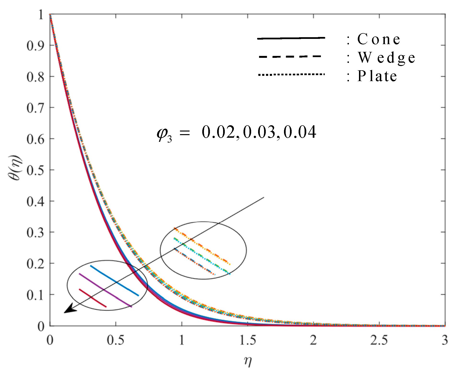
5.2. Discussion of Temperature Profiles

Figure 10, Figure 11, Figure 12, Figure 13, Figure 14 and Figure 15 show the influence of heat source/sink parameter Q, NVF $\varphi$, thermal radiation parameter R_d, suction/injection parameter Su, thermal relaxation parameter ${\gamma }_t$, and natural convection parameter $\lambda$ on the temperature $\theta$, respectively. Figure 10 displays that the temperature $\theta$ of the THNF is ominously affected by the heat source/sink parameter Q values. The temperature $\theta$ increases on increasing the value of parameter Q. The negative (Q < 0) and positive (Q > 0) values of parameter Q depict the mechanism of a heat sink and source, respectively.

The results depict that on amplifying the magnitude of the heat sink in the model, the temperature $\theta$ of THNF flow falls. The reason for the falling temperature is that the heat sink absorbs the heat produced in the BLR during the flow, which results in a falling temperature. Figure 11, Figure 12 and Figure 13 display the temperature $\theta$ of THNF with a rise in the NVF ${\varphi }_i$ of the NPs. The increasing NVF ${\varphi }_1$ of Al₂O₃ nanoparticles in the working fluid causes the temperature $\theta$ to increase. In addition, the increasing NVF ${\varphi }_2$ and ${\varphi }_3$ of Cu and CNT nanoparticles results in a decrease in temperature $\theta$. The increase in temperature due to an increase in NVF of Al₂O₃ nanoparticles is due to the spherical shape of these NPs, as the spherical shape has a larger surface area for interacting with other NPs, and due to this, the effective viscosity of THNF increases and a greater amount of heat is released. Consequently, the temperature $\theta$ of THNF increases with an increment in the NVF of Al₂O₃ nanoparticles. Figure 14 displays that the temperature $\theta$ of THNF surges with intensification in the radiation parameter R_d. This means that the radiation provides energy to the fluid particles, which surges their movement, and hence, the temperature rise. Furthermore, it is also seen that the temperature $\theta$ of the THNF is considerably affected by the radiation parameter R_d, which confirms its crucial role in the heat transmission process.

Figure 15 displays that the temperature $\theta$ of THNF falls with a rise in the numerical value of the suction/injection parameter Su. The increasing suction at the surface causes the width of the momentum boundary layer to reduce; consequently, the layers of the flow with zero momentum are provided energy, and they gain momentum and start their motion again. This process destroys the flow and reduces the friction at the boundary layer due to layers with zero momentum. Consequently, the temperature falls. Figure 16 displays that the temperature $\theta$ of THNF falls for higher estimates of the thermal relaxation parameter ${\gamma }_t$. The nonzero parameter ${\gamma }_t$ denotes lag in the heat conduction. The zero value of the parameter ${\gamma }_t$ resembles the traditional Fourier’s law for heat conduction. The higher values of the parameter ${\gamma }_t$ resemble the increased amount of time during the heat conduction. This revelation character of the Cattaneo–Christov model differentiates it from the “Fourier law of heat conduction”. The results indicate that increasing time lag during the heat transfer leads to lower temperature. Figure 17 displays that the temperature $\theta$ of THNF decreases with an increment in the natural convection parameter $\lambda$. The natural convection phenomenon is the mechanism of transportation of heat. This phenomenon causes THNF motion because of variation in fluid density, which occurs due to temperature gradients. The increasing temperature gradients cause the temperature to fall.

In Figure 10, Figure 11, Figure 12, Figure 13, Figure 14, Figure 15, Figure 16 and Figure 17, it is perceived that the temperature $\theta$ of THNF flow is highest for the flat plate and is lowest for the flow toward the cone. The flat surface of the plate allows the smooth motion of the flow and the increasing interaction of the NPs and working fluid particles, causing the system to interact properly, and consequently, the temperature rises. However, the curved surface of the cone obstructs the movement and the interaction of particles, and hence, the temperature is comparatively low for the flow toward the cone.

5.3. Discussion of Nanoparticles Concentration and Microorganisms Concentration

Figure 18, Figure 19 and Figure 20 show the influence of the Lewis number Le, suction/injection parameter Su, and solutal relaxation parameter ${\gamma }_c$ on the concentration $\varphi$ of NPs, respectively. Figure 18 shows the fall in the concentration of NPs with a rise in the Lewis number Le. The Lewis number Le is negatively correlated with molecular diffusivity. The increment in the Lewis number Le is seen as the lower molecular diffusivity. The lower diffusivity of the NPs in the BLR causes a fall in the concentration of NPs. Figure 19 displays that the NPs concentration is negatively correlated to the suction/injection parameter. Stronger suction at the surface destroys the flow and momentum, reducing the diffusivity of the NPs. Hence, the concentration falls due to the stronger suction.

Figure 20 depicts the influence of the solutal relaxation parameter ${\gamma }_c$ on concentration of NPs, and ${\gamma }_c\ne 0$ signifies the manifestation of lag in mass transfer. The zero value of parameter ${\gamma }_c$ corresponds to the traditional Fick’s law for mass diffusion. The higher values of the parameter ${\gamma }_c$ resemble the increased amount of time during the mass diffusion. Results depict that the higher estimates of parameter ${\gamma }_c$ lead NPs’ concentration to rise.

Figure 21, Figure 22, Figure 23 and Figure 24 depict the fluctuation of the microorganism concentration profile $\zeta \left(\eta \right)$ with the bioconvection Lewis number Lb, bioconvection Peclet number Pe, bioconvection constant $\varpi$, and suction/injection parameter Su. Figure 21, Figure 22 and Figure 23 show that the microorganism concentration profile $\zeta \left(\eta \right)$ falls with higher estimates of the bioconvection Lewis number Lb, Peclet number Pe, and bioconvection constant. The bioconvection Lewis number Lb is in charge of the system’s bioconvection. It increases heat diffusivity at the surface, lowering the density of microbes. It also diminishes the width of the boundary layer, which is proportional to the density of the motile microbe. Figure 24 shows that a rise in the suction/injection parameter Su causes the microorganism concentration profile $\zeta \left(\eta \right)$ to decrease. A stronger effect of the suction/injection parameter reduces the width of momentum and the NPs’ concentration boundary layer; as a result, the movement of layers and particles reduces, and it further causes the obstruction in the movement of the microorganism. Consequently, the microorganism concentration profile $\zeta \left(\eta \right)$ falls with increasing application of suction at the surface. In Figure 18, Figure 19, Figure 20, Figure 21, Figure 22, Figure 23 and Figure 24, it is observed that the concentration of NPs and microorganism concentration is highest for the flow toward the flat plate and is lowest for the flow toward the cone. The flat surface of the plate allows the smooth motion of the flow, and more and more diffusion of the NPs occurs; similarly, it also provides the smooth functioning of the microorganisms’ movement. However, the curved surface of the cone obstructs the diffusion of NPs and microorganisms’ movement; hence, these two profiles are comparatively low for the flow toward the cone.

5.4. Discussion of Nusselt Number, Sherwood Number, and Motile Microorganisms’ Density Gradient

Table 4. Numerical values of the Nusselt number (Nu), Sherwood number (Sh), and motile microorganisms’ density gradient (Nm).

										Cone $\left(n=1, \alpha =\frac{\pi }{4}\right)$			Wedge $\left(n=0, \alpha =\frac{\pi }{4}\right)$			Plate $\left(n=0, \alpha =0\right)$
Pe	$\varpi$	${\gamma }_t$	${\gamma }_{\mathrm{C}}$	Le	Lb	$\lambda$	Q	Rd	S	Nu	Sh	Nm	Nu	Sh	Nm	Nu	Sh	Nm
0.1	0.2	1.5	0.01	1.5	0.5	0.2	−2	10	0.1	24.92767	−1.51382	−0.87947	23.00199	−1.09132	−0.6332	23.02106	−1.09284	−0.63419
0.2										-	-	−1.03107	-	-	−0.74255	-	-	−0.74368
0.4										-	-	−1.33868	-	-	−0.96453	-	-	−0.96592
0.1	0.7									-	-	−0.93948	-	-	−0.67622	-	-	−0.67727
	1.7									-	-	−1.0595	-	-	−0.76227	-	-	−0.76342
	0.2	0.9								20.81458	−1.51501	−0.88056	19.29351	−1.09256	−0.63414	19.31295	−1.09457	−0.63551
		1.3								23.60737	−1.51414	−0.87976	21.80354	−1.09167	−0.63346	21.82288	−1.09332	−0.63456
		1.5	0.06							-	−1.38953	−0.86634	-	−1.04645	−0.62838	-	−1.04774	−0.62935
			0.16							-	−1.16796	−0.84311	-	−0.96177	−0.6193	-	−0.96266	−0.62024
			0.01	2						-	−1.81643	−0.91215	-	−1.3191	−0.65807	-	−1.32073	−0.65908
				3						-	−2.3356	−0.96938	-	−1.71464	−0.70207	-	−1.71641	−0.70309
				1.5	0.6					-	-	−0.97675	-	-	−0.69807	-	-	−0.69919
					0.7					-	-	−1.06895	-	-	−0.76131	-	-	−0.76253
					0.5	−1.8				24.55437	−1.47761	−0.85227	22.49837	−1.04949	−0.60575	22.28255	−1.03021	−0.59317
						2.2				25.26119	−1.5448	−0.90259	23.4335	−1.12445	−0.65503	23.61331	−1.13766	−0.66375
						0.2	−1.4			21.88554	−1.51457	−0.88013	20.27092	−1.09219	−0.63385	20.294	−1.09404	−0.6351
							−0.8			18.43186	−1.51581	−0.88131	17.15315	−1.09365	−0.63502	17.18372	−1.09606	−0.63672
							0.4			7.816058	−1.53274	−0.90268	7.173743	−1.11078	−0.65175	7.408173	−1.11788	−0.65803
							−2	12		26.66715	−1.51439	−0.87998	24.58693	−1.09197	−0.63368	24.61154	−1.09374	−0.63487
								14		28.25102	−1.51495	−0.88049	26.03504	−1.0926	−0.63417	26.06564	−1.09462	−0.63555
								16		29.70916	−1.51549	−0.88101	27.37275	−1.09321	−0.63465	27.40974	−1.09547	−0.63623
								10	−0.1	22.27847	−1.287	−0.77905	19.99349	−0.85639	−0.53176	20.0157	−0.85824	−0.53294
									0.1	24.92767	−1.51382	−0.87947	23.00199	−1.09132	−0.6332	23.02106	−1.09284	−0.63419
									0.3	27.94773	−1.7543	−0.98592	26.47821	−1.3467	−0.74315	26.49433	−1.3479	−0.74397

and

Table 5. Numerical values of the Nusselt number (Nu), Sherwood number (Sh), and motile microorganisms’ density gradient (Nm) for volume fraction of nanoparticles.

.			Cone $\left(n=1, \alpha =\frac{\pi }{4}\right)$			Wedge $\left(n=0, \alpha =\frac{\pi }{4}\right)$			Plate $\left(n=0, \alpha =0\right)$
${\phi }_1$	${\phi }_2$	${\phi }_3$	Nu	Sh	Nm	Nu	Sh	Nm	Nu	Sh	Nm
0.02	0.02	0.02	24.92767	−1.51382	−0.87947	23.00199	−1.09132	−0.6332	23.02106	−1.09284	−0.63419
0.03			24.84579	−1.41239	−0.8171	22.92604	−1.01785	−0.58918	22.94572	−1.01933	−0.59014
0.04			24.78749	−1.33885	−0.77203	22.87163	−0.96459	−0.55737	22.89167	−0.96603	−0.5583
0.02	0.03		25.06144	−1.67807	−0.98093	23.12018	−1.21024	−0.7047	23.13655	−1.21166	−0.70564
	0.04		25.26947	−1.98846	−1.17404	23.30667	−1.43523	−0.84079	23.31994	−1.43655	−0.84169
	0.02	0.03	25.15922	−1.86527	−1.09724	23.20391	−1.346	−0.78672	23.21942	−1.34746	−0.78771
		0.04	25.4086	−2.36089	−1.40762	23.42386	−1.70561	−1.00551	23.43616	−1.70703	−1.00649

display the influence of flow parameters on the Nusselt (Nu) number depicting HT rate, Sherwood (Sh) number depicting mass transmission rate (MT rate), and microorganisms’ density gradient (Nm) at the surface. Figure 25 is drawn to present the variation in Nusselt number (Nu). The higher estimates of the natural convection parameter $\lambda$ cause the HT rate to rise, whereas the MT rate and microorganisms’ density gradient fall. The rising natural convection phenomenon causes the HT rate to rise due to the transportation of heat. This phenomenon causes THNF motion because of variation in fluid density, which occurs due to temperature gradients. The increasing magnitude of the suction parameter Su and heat sink parameter Q (Q < 0) acts to increase the HT rate. The magnification in the HT rate is due to a reduction in thermal BLR thickness. The reduced thickness allows more transmission of heat through the surface. On the contrary, the increasing suction parameter causes the MT rate and microorganisms’ density gradient (Nm) to decrease. Higher estimates of the radiation parameter R_d increase the HT rate. This means that the radiation provides energy to the particles, which surges their movement and, hence, the interaction with other particles, causing the HT rate to rise.

On increasing the NVF ${\phi }_2$ and ${\phi }_3$ of Cu and CNT nanoparticles, the HT rate rises, but on the contrary, on increasing the NVF ${\phi }_1$ of Al₂O₃ nanoparticles, the HT rate decreases. This is because of the fact that when increasing the NVF of Cu and CNT nanoparticles, thermal boundary layer thickness decreases, whereas on increasing the NVF of Al₂O₃ nanoparticles, thermal boundary layer thickness increases. The reduction in thermal boundary layer thickness causes a greater amount of heat to transfer through the surface. Consequently, the HT rate increases. The amplification of the thermal relaxation parameter ${\gamma }_t$ causes the HT rate to increase at the surface. This result implies that the higher time lag present during the transmission causes an enhanced HT rate. Furthermore, higher solutal relaxation parameter ${\gamma }_c$ acts to increase the MT rate and microorganisms’ density gradient (Nm). This implies that a higher time lag during the mass transmission causes an enhanced MT rate, and it also helps the microorganisms’ density to increase. The rising Lewis number acts to decrease the MT rate and microorganisms’ density gradient (Nm). In addition, bioconvection Peclet number Pe, bioconvection constant $\varpi$, and bioconvection Lewis number Lb are negatively correlated with the microorganisms’ density gradient (Nm). The results depict that the heat transmission rate is highest for the flow toward the cone, whereas the mass transmission rate and microbe density gradient are highest for the flow toward the wedge.

6. Conclusions

This paper deals with the bioconvective 2D THNF flow (Al₂O₃-Cu-CNT/water flow) containing a microbial suspension toward three different geometries (a flat plate, a wedge, and a cone) with the suction/injection effect. The Cattaneo–Christov theory is used to analyze HT rate and MT rate. The THNF flow is modeled bearing in mind the effects of natural convection, radiation, and heat source/sink. The in-built function “bvp4c in MATLAB” is used to solve the equations, and the solutions are shown in graphs. The key findings of the study are:

➢

A stronger application of suction causes the thickness of the momentum boundary layer to reduce.

➢

The temperature of THNF increases with higher radiation parameter and heat source/sink parameter.

➢

The increasing value of the thermal relaxation parameter corresponding to the Cattaneo–Christov theory acts to enhance the heat transmission rate.

➢

The microorganism concentration profile decreases with higher bioconvection Lewis number.

➢

The heat transmission rate is highest for the flow toward the cone.

➢

Mass transmission rate and microbe density gradient are highest for the flow toward the wedge.

Future Scope of Research

The present study discusses the flow of ternary hybrid nanofluid without the nanoparticle aggregation effect. The study can be extended for nanoparticle aggregation effect with proper modeling of fluid flow by utilization of validated thermophysical correlations.

References

1. Choi, S.U.S. Enhancing Thermal Conductivity of Fluids with Nanoparticles. Am. Soc. Mech. Eng. Fluids Eng. Div. FED 1995, 231, 99–105. [Google Scholar]
2. Sahoo, R.R. Thermo-Hydraulic Characteristics of Radiator with Various Shape Nanoparticle-Based Ternary Hybrid Nanofluid. Powder Technol. 2020, 370, 19–28. [Google Scholar] [CrossRef]
3. Adun, H.; Kavaz, D.; Dagbasi, M. Review of Ternary Hybrid Nanofluid: Synthesis, Stability, Thermophysical Properties, Heat Transfer Applications, and Environmental Effects. J. Clean. Prod. 2021, 328, 129525. [Google Scholar] [CrossRef]
4. Xuan, Z.; Zhai, Y.; Ma, M.; Li, Y.; Wang, H. Thermo-Economic Performance and Sensitivity Analysis of Ternary Hybrid Nanofluids. J. Mol. Liq. 2021, 323, 114889. [Google Scholar] [CrossRef]
5. Sahoo, R.R.; Kumar, V. Development of a New Correlation to Determine the Viscosity of Ternary Hybrid Nanofluid. Int. Commun. Heat Mass Transf. 2020, 111, 104451. [Google Scholar] [CrossRef]
6. Sahoo, R.R. Experimental Study on the Viscosity of Hybrid Nanofluid and Development of a New Correlation. Heat Mass Transf. 2020, 56, 3023–3033. [Google Scholar] [CrossRef]
7. Animasaun, I.L.; Yook, S.J.; Muhammad, T.; Mathew, A. Dynamics of Ternary-Hybrid Nanofluid Subject to Magnetic Flux Density and Heat Source or Sink on a Convectively Heated Surface. Surf. Interfaces 2022, 28, 101654. [Google Scholar] [CrossRef]
8. Alanazi, M.M.; Ahmed Hendi, A.; Ahammad, N.A.; Ali, B.; Majeed, S.; Shah, N.A. Significance of Ternary Hybrid Nanoparticles on the Dynamics of Nanofluids over a Stretched Surface Subject to Gravity Modulation. Mathematics 2023, 11, 809. [Google Scholar] [CrossRef]
9. Raju, C.S.K.; Ameer, N.A.; Kiran, S.; Nehad, A.S.; Se-jin, Y.; Dinesh, M.K. Nonlinear linear movements of axisymmetric ternary hybrid nanofluids in a thermally radiated expanding or contracting permeable Darcy Walls with different shapes and densities: Simple linear regression. Int. Commun. Heat Mass Transfer 2022, 135, 106110. [Google Scholar] [CrossRef]
10. Ramzan, M.; Dawar, A.; Saeed, A.; Kumam, P.; Sitthithakerngkiet, K.; Lone, S.A. Analysis of the Partially Ionized Kerosene Oil-Based Ternary Nanofluid Flow over a Convectively Heated Rotating Surface. Open Phys. 2022, 20, 507–525. [Google Scholar] [CrossRef]
11. Fourier, J. Théorie Analytique de La Chaleur; Chez Firmin Didot: Paris, France, 1822. [Google Scholar]
12. Cattaneo, C. Sulla Conduzione Del Calore. Atti Sem. Mat. Fis. Univ. Modena 1948, 3, 83–101. [Google Scholar]
13. Christov, C.I. On Frame Indifferent Formulation of the Maxwell-Cattaneo Model of Finite-Speed Heat Conduction. Mech. Res. Commun. 2009, 36, 481–486. [Google Scholar] [CrossRef]
14. Venkateswarlu, S.; Varma, S.V.K.; Durga Prasad, P. MHD Flow of MoS2 and MgO Water-Based Nanofluid through Porous Medium over a Stretching Surface with Cattaneo-Christov Heat Flux Model and Convective Boundary Condition. Int. J. Ambient Energy 2020, 43, 2940–2949. [Google Scholar] [CrossRef]
15. Rawat, S.K.; Kumar, M. Cattaneo–Christov Heat Flux Model in Flow of Copper Water Nanofluid Through a Stretching/Shrinking Sheet on Stagnation Point in Presence of Heat Generation/Absorption and Activation Energy. Int. J. Appl. Comput. Math. 2020, 6, 112. [Google Scholar] [CrossRef]
16. Ramzan, M.; Gul, H.; Baleanu, D.; Nisar, K.S.; Malik, M.Y. Role of Cattaneo–Christov Heat Flux in an MHD Micropolar Dusty Nanofluid Flow with Zero Mass Flux Condition. Sci. Rep. 2021, 11, 19528. [Google Scholar] [CrossRef]
17. Lv, Y.P.; Gul, H.; Ramzan, M.; Chung, J.D.; Bilal, M. Bioconvective Reiner–Rivlin Nanofluid Flow over a Rotating Disk with Cattaneo–Christov Flow Heat Flux and Entropy Generation Analysis. Sci. Rep. 2021, 11, 15859. [Google Scholar] [CrossRef]
18. Abderrahmane, A.; Qasem, N.A.A.; Younis, O.; Marzouki, R.; Mourad, A.; Shah, N.A.; Chung, J.D. MHD Hybrid Nanofluid Mixed Convection Heat Transfer and Entropy Generation in a 3-D Triangular Porous Cavity with Zigzag Wall and Rotating Cylinder. Mathematics 2022, 10, 769. [Google Scholar] [CrossRef]
19. Kumar, M.D.; Raju, C.S.K.; Sajjan, K.; El-Zahar, E.R.; Shah, N.A. Linear and quadratic convection on 3D flow with transpiration and hybrid nanoparticles. Int. Commun. Heat Mass Transfer 2022, 134, 105995. [Google Scholar] [CrossRef]
20. Sajjan, K.; Shah, N.A.; Ahammad, N.A.; Raju, C.S.K.; Kumar, M.D.; Weera, W. Nonlinear Boussinesq and Rosseland approximations on 3D flow in an interruption of Ternary nanoparticles with various shapes of densities and conductivity properties. AIMS Math. 2022, 7, 18416–18449. [Google Scholar] [CrossRef]
21. Kuznetsov, A.V. Bio-Thermal Convection Induced by Two Different Species of Microorganisms. Int. Commun. Heat Mass Transf. 2011, 38, 548–553. [Google Scholar] [CrossRef]
22. Shi, Q.-H.H.; Hamid, A.; Khan, M.I.; Kumar, R.N.; Gowda, R.J.P.P.; Prasannakumara, B.C.; Shah, N.A.; Khan, S.U.; Chung, J.D.; Naveen Kumar, R.; et al. Numerical Study of Bio-Convection Flow of Magneto-Cross Nanofluid Containing Gyrotactic Microorganisms with Activation Energy. Sci. Rep. 2021, 11, 16030. [Google Scholar] [CrossRef] [PubMed]
23. Al-Khaled, K.; Ullah Khan, S. Thermal Aspects of Casson Nanoliquid with Gyrotactic Microorganisms, Temperature-Dependent Viscosity, and Variable Thermal Conductivity: Bio-Technology and Thermal Applications. Inventions 2020, 5, 39. [Google Scholar] [CrossRef]
24. Bhatti, M.M.; Marin, M.; Zeeshan, A.; Ellahi, R.; Abdelsalam, S.I. Swimming of Motile Gyrotactic Microorganisms and Nanoparticles in Blood Flow Through Anisotropically Tapered Arteries. Front. Phys. 2020, 8, 95. [Google Scholar] [CrossRef] [Green Version]
25. Kairi, R.R.; Shaw, S.; Roy, S.; Raut, S. Thermosolutal Marangoni Impact on Bioconvection in Suspension of Gyrotactic Microorganisms over an Inclined Stretching Sheet. J. Heat Transf. 2021, 143, 031201. [Google Scholar] [CrossRef]
26. Ali, A.; Sarkar, S.; Das, S.; Jana, R.N. Investigation of Cattaneo–Christov Double Diffusions Theory in Bioconvective Slip Flow of Radiated Magneto-Cross-Nanomaterial Over Stretching Cylinder/Plate with Activation Energy. Int. J. Appl. Comput. Math. 2021, 7, 208. [Google Scholar] [CrossRef]
27. Mishra, A.; Kumar, M. Numerical Analysis of MHD Nanofluid Flow over a Wedge, Including Effects of Viscous Dissipation and Heat Generation/Absorption, Using Buongiorno Model. Heat Transf. 2021, 50, 8453–8474. [Google Scholar] [CrossRef]
28. Yaseen, M.; Rawat, S.K.; Kumar, M. Falkner–Skan Problem for a Stretching or Shrinking Wedge With Nanoparticle Aggregation. J. Heat Transf. 2022, 144, 102501. [Google Scholar] [CrossRef]
29. Mahanthesh, B.; Mackolil, J. Flow of Nanoliquid Past a Vertical Plate with Novel Quadratic Thermal Radiation and Quadratic Boussinesq Approximation: Sensitivity Analysis. Int. Commun. Heat Mass Transf. 2021, 120, 105040. [Google Scholar] [CrossRef]
30. Gumber, P.; Yaseen, M.; Kumar, S.; Kumar, M. Heat Transfer in Micropolar Hybrid Nanofluid Flow Past a Vertical Plate in the Presence of Thermal Radiation and Suction/Injection Effects. Partial Differ. Equ. Appl. Math. 2022, 5, 100240. [Google Scholar] [CrossRef]
31. Rawat, S.K.; Upreti, H.; Kumar, M. Comparative Study of Mixed Convective MHD Cu-Water Nanofluid Flow over a Cone and Wedge Using Modified Buongiorno’s Model in Presence of Thermal Radiation and Chemical Reaction via Cattaneo-Christov Double Diffusion Model. J. Appl. Comput. Mech. 2021, 7, 1383–1402. [Google Scholar] [CrossRef]
32. Sandeep, N.; Reddy, M.G. Heat Transfer of Nonlinear Radiative Magnetohydrodynamic Cu-Water Nanofluid Flow over Two Different Geometries. J. Mol. Liq. 2017, 225, 87–94. [Google Scholar] [CrossRef]
33. Reddy, M.G.; Rani, M.V.V.N.L.S.; Kumar, K.G.; Prasannakumara, B.C. Cattaneo–Christov Heat Flux and Non-Uniform Heat-Source/Sink Impacts on Radiative Oldroyd-B Two-Phase Flow across a Cone/Wedge. J. Braz. Soc. Mech. Sci. Eng. 2018, 40, 95. [Google Scholar] [CrossRef]
34. Jayachandra Babu, M.; Sandeep, N.; Saleem, S. Free Convective MHD Cattaneo-Christov Flow over Three Different Geometries with Thermophoresis and Brownian Motion. Alex. Eng. J. 2017, 56, 659–669. [Google Scholar] [CrossRef]
35. Garia, R.; Rawat, S.K.; Kumar, M.; Yaseen, M. Hybrid Nanofluid Flow over Two Different Geometries with Cattaneo–Christov Heat Flux Model and Heat Generation: A Model with Correlation Coefficient and Probable Error. Chin. J. Phys. 2021, 74, 421–439. [Google Scholar] [CrossRef]
36. Arif, M.; Kumam, P.; Kumam, W.; Mostafa, Z. Heat Transfer Analysis of Radiator Using Different Shaped Nanoparticles Water-Based Ternary Hybrid Nanofluid with Applications: A Fractional Model. Case Stud. Therm. Eng. 2022, 31, 101837. [Google Scholar] [CrossRef]
37. Elnaqeeb, T.; Animasaun, I.L.; Shah, N.A. Ternary-Hybrid Nanofluids: Significance of Suction and Dual-Stretching on Three-Dimensional Flow of Water Conveying Nanoparticles with Various Shapes and Densities. Z. Naturforsch.—Sect. A J. Phys. Sci. 2021, 76, 231–243. [Google Scholar] [CrossRef]
38. Vajravelu, K.; Nayfeh, J. Hydromagnetic Convection at a Cone and a Wedge. Int. Commun. Heat Mass Transf. 1992, 19, 701–710. [Google Scholar] [CrossRef]
39. Yaseen, M.; Rawat, S.K.; Kumar, M. Cattaneo–Christov Heat Flux Model in Darcy–Forchheimer Radiative Flow of MoS2–SiO2/Kerosene Oil between Two Parallel Rotating Disks. J. Therm. Anal. Calorim. 2022, 147, 10865–10887. [Google Scholar] [CrossRef]
40. Shampine, L.F.; Gladwell, I.; Thompson, S. Solving ODEs with MATLAB; Cambridge University Press: Cambridge, UK, 2003; ISBN 9780511615542. [Google Scholar]
Figure 1. Physical model.
Mathematics 11 01237 g001
Figure 2. Flow chart.
Mathematics 11 01237 g002
Figure 3. Effect of λ on f ( η ) .
Mathematics 11 01237 g003
Figure 4. Effect of φ 1 on f ( η ) .
Mathematics 11 01237 g004
Figure 5. Effect of φ 2 on f ( η ) .
Mathematics 11 01237 g005
Figure 6. Effect of φ 3 on f ( η ) .
Mathematics 11 01237 g006
Figure 7. Effect of Su on f ( η ) .
Mathematics 11 01237 g007
Figure 8. Velocity boundary layer patterns for (a) flat plate, (b) wedge, and (c) cone.
Mathematics 11 01237 g008aMathematics 11 01237 g008b
Figure 9. Streamlines for (a) flat plate, (b) wedge, and (c) cone.
Mathematics 11 01237 g009
Figure 10. Effect of Q on θ ( η ) .
Mathematics 11 01237 g010
Figure 11. Effect of φ 1 on θ ( η ) .
Mathematics 11 01237 g011
Figure 12. Effect of φ 2 on θ ( η ) .
Mathematics 11 01237 g012
Figure 13. Effect of φ 3 on θ ( η ) .
Mathematics 11 01237 g013
Figure 14. Effect of Rd on θ ( η ) .
Mathematics 11 01237 g014
Figure 15. Effect of Su on θ ( η ) .
Mathematics 11 01237 g015
Figure 16. Effect of γ t on θ ( η ) .
Mathematics 11 01237 g016
Figure 17. Effect of λ on θ ( η ) .
Mathematics 11 01237 g017
Figure 18. Effect of Le on ϕ ( η ) .
Mathematics 11 01237 g018
Figure 19. Effect of Su on ϕ ( η ) .
Mathematics 11 01237 g019
Figure 20. Effect of γ c on ϕ ( η ) .
Mathematics 11 01237 g020
Figure 21. Effect of Lb on ζ ( η ) .
Mathematics 11 01237 g021
Figure 22. Effect of Pe on ζ ( η ) .
Mathematics 11 01237 g022
Figure 23. Effect of Su on ζ ( η ) .
Mathematics 11 01237 g023
Figure 24. Effect of ϖ on ζ ( η ) .
Mathematics 11 01237 g024
Figure 25. Nusselt number (a) flat plate, (b) wedge, and (c) cone.
Mathematics 11 01237 g025aMathematics 11 01237 g025b