
Confluence Effect of Debris-Filled Damage and Temperature Variations on Guided-Wave Ultrasonic Testing (GWUT)


School of Aerospace, Transport and Manufacturing, Cranfield University, Bedford MK43 0AL, UK
*
Author to whom correspondence should be addressed.
Processes 2024, 12(5), 957; https://doi.org/10.3390/pr12050957
Submission received: 30 March 2024
/
Revised: 16 April 2024
/
Accepted: 27 April 2024
/
Published: 8 May 2024
(This article belongs to the Special Issue Industrial Process Operation State Sensing and Performance Optimization)
Abstract
:Continuous monitoring of structural health is essential for the timely detection of damage and avoidance of structural failure. Guided-wave ultrasonic testing (GWUT) assesses structural damages by correlating its sensitive features with the damage parameter of interest. However, few or no studies have been performed on the detection and influence of debris-filled damage on GWUT under environmental conditions. This paper used the pitch–catch technique of GWUT, signal cross-correlation, statistical root mean square (RMS) and root mean square deviation (RMSD) to study the combined influence of varying debris-filled damage percentages and temperatures on damage detection. Through experimental result analysis, a predictive model with an R2 of about 78% and RMSE values of about was established. When validated, the model proved effective, with a comparable relative error of less than 10%.
1. Introduction
High economic structural assets in aerospace, shipbuilding, oil, and gas are constructed using thin-wall metallic materials. The structural assets convey products prone to environmental hazards that could happen through structural failure [1,2]. Failures in structures are deeply traced to undetected damage. Cracks and corrosion are forms of damage that are mainly studied individually using guided-wave ultrasonics [3]. Damage is a state of structure that differs from its pristine state [4]. It is an indispensable factor affecting the structure’s service lifecycle and its reliability for intended operational services. Damage may be initiated in structural material during the manufacturing process at the micro-level and progresses into the macro-level during the service time of the structure. Formed damage, such as a crack in structures, could accumulate debris over time and accelerate structure deterioration, paving the way for catastrophic failure. The accumulated debris causes crack closure, affects crack propagation and enhances pitting corrosion activities, as explained in [5,6]. The prime effects of corrosion and crack on metallic structures are thickness thinning, rigidity reduction, integrity and load-carrying-capacity degradation [7], shortening the structure’s service lifecycle and making it unreliable. Hence, continuous monitoring of the structural assets with cost-effective damage-sensitive NDT devices and techniques is a priority to avert catastrophic failure, suggest timely maintenance, and save the economy. Most of the previous studies have been on the monitoring and prediction of empty cracks (cracks without debris or dry cracks) in structures using various structural health-monitoring techniques [8,9,10,11,12,13,14]. In recent decades, the guided-wave ultrasonic technique has received more attention than other NDT techniques for SHM [15]. The high interest in GWUT is due to its potential for long-range inspection, non-invasive inspection, the lightweight and small size of the ceramic PZT, and cost-effectiveness. It has been successfully used for the detection and localisation of various damages in structures [9,15,16,17,18]. The effect of environmental and operational conditions on the ultrasonic guided wave, especially temperature, has been well studied [19,20]. However, the influence of debris-filled damage cum temperature variation on the guided wave has not been studied. The influence of debris-filled damage of different percentages under temperature variation is meticulously studied in this paper using statistical RMS and RMSD of the captured response signals from the pitch–catch ultrasonic guided-wave configuration. The suitability of RMS is because the guided-wave ultrasonic used in SHM is a continuous propagation of energy from one point of the structure to another. And, the sensitivity of the signal’s energy to damage is significantly higher than the amplitude, since it is the square of amplitude by value.
2. Theory
2.1. Structural Health Monitoring (SHM)
Structural health monitoring (SHM) via an ultrasonic guided wave uses an embedded ceramic piezoelectric (PZT) transducer to transform an oscillating excitation signal into an actuating signal that would cause a stress wave to propagate in the host structure through surface pinching. The propagating wave interacts with the structure and becomes captured as a response signal by another ceramic PZT called a sensor [21]. The PZT operates through a linear transduction mechanism as expressed in the linear constitutive equations in [9,15].
where and , are the strain and stress mechanical variables, respectively. and , are electrical displacement and electrical field variables, respectively. , is the mechanical compliance at zero electric fields, , is the dielectric constant at zero mechanical stress, and and , denote a coupling between the electrical and mechanical variables. Equations (1) and (2) are actuation and sensing equations. Hence, the sensor PZT captures the strain effect of the propagating stress wave and transforms it into a signal voltage. The sensor’s output voltage is proportional to the amount of the strain effect caused by the propagating wave and the thickness of the sensor.
2.2. Wave Motion in Thin Plate
The ultrasonic wave propagates as a distributed stress on a thin plate. The stress causes material particles to vibrate and transfer energy from one point to another as waves. The waves are guided to propagate within the boundaries of the structure. The motion of the vibrating particle in the plate is governed by Equation (3). The boundary condition of surface traction force is in Equation (4).
where is the displacement of the plate via the particle motion, and are Lame’s constants, is the density of the plate particles, is the acceleration of the vibrating particles, is the force body on the material, is surface tractions at the normal , and , is the stress on the plate surface. It is considered zero for a traction-free body condition. The solution to Equation (3) by the method of potential separation, as in [22], results in characteristics frequency equations of lamb wave grouped into two modes as in Equations (5) and (6). The terms of the equations are as expanded in Equations (7) through (9).
where
The velocity of the propagating wave is related to the lame’s constant and mechanical properties of the material, as expressed in Equations (10) and (11).
where is the transverse velocity, and is the longitudinal or radial velocity of the wave in a solid medium. is the phase velocity of lamb wave, and and are the material density, elastic modulus, and Poison ratio, respectively. It is pertinent to observe that the velocity of the propagating wave depends on the mechanical properties of the waveguide. Hence, any consequential effect on the material would affect sensitive parameters of the propagating wave, especially its energy being transferred as the wave propagates.
2.3. Wave Dispersion Curve
In an active structural health-monitoring (SHM) mode, the actuator pinches the structure to create probing waves when excited with an oscillating electrical voltage. The frequency of the probing signal is often selected from the dispersion curve. The dispersion curves are a set of curves that represent the propagation of wave modes in each waveguide. It describes the relationship between wave velocity (group or phase) and the excitation frequency [18]. The dispersion curve is determined using Disperse software or a Dispersion calculator versionV2.3 by providing the necessary properties of the plate material [23]. The dispersion curves of the 3.00 mm mild carbon steel plate with properties listed in Table 1 are in Figure 1.
From the dispersion curves, only the fundamental modes exist when the frequency is below 500 KHz, but beyond it, multi-modes exist. Also, the fundamental symmetric mode possesses higher velocity, which is relatively more constant at the early frequency range than the fundamental asymmetric mode. The selection of probing frequency is critical for damage detection. There are some criteria used to select an appropriate probing frequency. One of the criteria is that the frequency must be sensitive to the targeted damage and possess enough energy to propagate the needed distance. An excitation frequency with the largest RMS is selected through experimental frequency sweep because it possesses more energy than any other and could travel the longest distance. Recall the rule of thumb for damage detection, which states that damage would stand a higher chance of detection if it is larger than of the probing wave [24]. Hence, it is necessary to compare the probing wave’s wavelength with the targeted damage’s length. The wavelength of the excitation frequency can be determined using Equation (13).
2.4. Wave–Damage Interaction Effects and Inspection-Transducer Configuration
Guided-wave ultrasonic inspection could be performed using active or passive ultrasonic configuration techniques. The exciter is vital in guided-wave inspection, which determines if a configuration is active or passive. When damage generates the propagating wave, a passive mode is configured [21], and all the embedded transducers would function like human ears and listen to pick up the wave. The active mode is configured when the propagating wave is due to the excitation of the actuator with an oscillating electrical voltage of a given frequency [21,25,26,27]. The vibration of the actuator causes atoms of the structure around its installation to start displacing their positions temporarily. This mechanism transfers wave energy from one point of the structure to another. The propagating stress wave is constrained by the boundaries of the structure (waveguide), hence the guided wave. The wave interaction with the structure, especially with damage or discontinuity, causes scattering, reflections, mode conversion, and some energy absorption at the damaged spot [28]. Figure 2b depicts the effect of wave–damage interaction. Figure 2b shows that the through-transmitted wave is much smaller than the edge-scattered wave. Hence, capturing the edge-scattered wave would be more valuable than the through-transmitted wave. Also, depending on the nature of the damage, the through transmitted is the resultant wave after absorption, back reflection, and diffraction of the incident wave, which is usually small in value.
All the effects mentioned above make it possible for damage to be detected and localised using guided-wave techniques and a sensitive wave parameter called the signature or feature. The extent of wave reflection or scattering depends on the encountered damage’s nature, shape, size, and orientation. Pitch–catch and Pulse–Echo transducer configuration topology are often used in the active-mode inspection technique, as shown in Figure 3. The choice of either topology depends on the nature of the damage. This study uses pitch–catch configuration topology to acquire wave signals interacting with the damaged and scattered.
2.5. Temperature Effect on Guided Wave
Damage and temperature affect mechanical structures differently but collectively influence structural degradation [29,30]. The core influence of temperature on a mechanical structure is thermal expansion and assisted degradation of the structure’s strength and stiffness. In particular, an increase in temperature causes a decrease in the elastic modulus of a metallic structure, and features of the propagating wave depend directly on most of the structure’s mechanical properties, especially the elastic modulus, as in Equations (10) and (11). Assuming a linear dependence of the wave characteristics on temperature, the equation below would be suitable for the study.
where
- = any characteristics parameter of the wave.
- = the value of the wave feature at a reference temperature.
- = current-state temperature of the structure.
- = reference temperature of the structure.
2.6. Signature/Wave Feature Extraction and Processing
Damage detection and identification largely depend on the approach and signal-processing technique adopted. The captured response signal carries sufficient information about the structure. Wave amplitude is one of the sensitive parameters of the wave and could be easily extracted from the signal. The damage in the structure could modulate the signal amplitude to either higher or lower values. However, the signal energy is more sensitive to damage and is proportional to the square of its amplitude. Hence, we adopted root mean square (RMS) and root mean square deviation (RMSD) to extract the energy feature of the response wave and determine the damage index. A model for predicting the debris-filled damage under temperature variation will be established through the extracted feature of the wave. The average RMS of the two sensors’ signals used in the design is given in Equation (15), and the relative RMS is expressed in Equation (16).
where
- = the RMS of the excitation signal.
- and are the captured response signals from PZT2 and PZT4, respectively.
N is the number of samples of the signal. Hence, the is computed for each study case and used to establish the predictive regression model for each damage situation. The damage index is computed by determining the RMSD between the healthy state of the structure and its damaged state. Equation (17) expresses the damage index.
where
is the relative RMS of the sensors’ captured response signals in the damaged state of the plate, while the is the healthy counterpart of the sensors’ response signals.
3. Materials and Methods
3.1. Material Preparation
The materials used in the study are mild carbon steel plates. Mild carbon steel has a low carbon percentage. It is tough and ductile, making it a predominantly used material to construct essential and critical structures of high economic value, such as oil and gas pipelines, rail tracks, and bridges. The dimensions of the mild carbon steel plate used in this study are . Damage of 40.00 mm length, 5.00 mm width, and varying depth of 1.00 mm to 2.50 mm at an interval of 0.50 mm, as depicted in Figure 4, was carefully machined at the mid-distance between the actuator, PZT1 and sensor, and PZT3. Circular PZT transducers were used due to their omnidirectional capability of radiating and receiving response signals, unlike rectangular PZTs, which are orientation dependent [31]. The variation in the damage depth was used to simulate the material-thinning thickness that corrosion activities would cause. Table 1 reveals the mechanical properties of the used plate material. Wave reflection from the edges of the plate is known to contribute to the complexity of the response wave. In particular, the edge-reflected wave would cause mutual interference with the response wave of the actuated signal. Hence, DAS modelling air-dried clay [32] is installed around the edges of the plate to absorb any wave reflection from it. Also, the transition of random vibration between the plate and the working table was minimised by placing soft foams between the two.
3.2. Experimental Setup
Pitch–catch configuration topology was adopted and implemented using four ceramic PZT transducers from Mouser Electronics, Wycombe, UK (PZT: ) as shown in Figure 4. A circular type of PZT transducer was used due to its omnidirectional capability in capturing response signals. Before transducers were installed, acetone was used to clean the plate’s surfaces, and it was allowed to dry up for about 10 min. The transducers were embedded on the top surface of the plate using epoxy adhesive. The curing time of the epoxy adhesive is 150 min and has an operating temperature range of −55 °C and 120 °C [33]. However, we allowed 180 min to ensure the proper curing of the adhesive. One transducer, PZT1, was wired as the actuator to generate the probing wave, while the remaining three transducers were used as sensors. The sensor PZTs were arranged and named as left sensor (PZT2), middle sensor (PZT3), and right sensor (PZT4) when viewed from the actuator’s position. The epoxy adhesive was lightly applied to bond the PZTs on the top surface of the plate and to eliminate the high impedance that air would have introduced. The properties of the ceramic PZTs are in Table 2. The PZTs are installed 102.00 mm from the end edges of the plate and at least 100.00 mm from the side edges. The PZT1 is 300.00 mm separated from the PZT3. The distance between the middle sensor, PZT3, and either of the two sensors is 50.00 mm. The excitation signal was generated using an arbitrary function generator (TG550 Function Generator), while the response signals were visualised and registered using an Agilent Technologies Mixed Signal Oscilloscope (MSO-X 3024A), with a sampling frequency of 1 MHz. The experiment study was conducted in 3 phases.
3.3. Study Phases
Phase I: To ensure that the testing rig works and proper excitation frequency is selected and used for the study, PZT1 was excited with different centre frequencies of an amplitude-modulated wave. The modulating frequency is internal 400 Hz of the arbitrary function generator, and the different centre frequencies are 100 KHz, 180 KHz, 280 KHz, and 360 KHz. Each modulated wave was used to excite the PZT1 5 times and averaged to ensure repeatability and minimise the random-noise effect. The signals captured by PZT2 and PZT4 were processed using Equations (15) and (16) to determine which excitation frequency offered the maximum signal energy. The signal captured by PZT3 was processed using the cross-correlation method to determine the time of flight () of the wave packets and compared it with the theoretically determined time of fight, ().
Phase II: The selected excitation frequency was used to acquire baseline signals by PZT2 and PZT4 under the influence and no influence of temperature on the wave signal at the healthy state of the plate. A silicone heat mat and K-type thermocouple temperature sensor were integrated into the testing rig to generate heat and acquire the plate’s temperature, respectively. A control circuitry was designed using Arduino Mega and solid-state relay (SSL) to regulate the heating rate of the silicone heat mat and ensure that the targeted temperature value was achieved and maintained before baseline response signals were acquired and recorded. The temperature was varied from 30 °C to 70 °C at an interval of 5 °C.
Phase III: After baseline signal acquisition, the healthy plate was replaced with an unhealthy plate that had damage dimensions, as depicted in Table 3. The response signals were captured by PZT2 and PZT4 after they had interacted with the following:
Empty damage at influence and no influence of temperature.
Damage filled with different percentages of corrosion debris at influence and no influence of temperature. The testing rig used is as in Figure 4 and Figure 5.

Table 3.
The damage dimension.
| S/N | Damage Depth (mm) | Damage Length (mm) | Damage Width (mm) |
|---|---|---|---|
| 1 | 1.00 | 40.00 | 5.00 |
| 2 | 1.50 | 40.00 | 5.00 |
| 3 | 2.00 | 40.00 | 5.00 |
| 4 | 2.50 | 40.00 | 5.00 |
4. Results
4.1. Excitation Frequency Selection
In structural health monitoring, SHM, inspection frequency is essential for detecting damage. As stated in Phase I, two approaches were used to determine the excitation frequency for the studies. In the first approach, PZT1 was excited with different centre frequency signals, and the corresponding response signals for each frequency were captured using the PZT2 and PZT4 sensors. The following four frequencies, 100 KHz, 180 KHz, 280 KHz, and 360 KHz, were used to excite the actuator. The response signals captured by the sensors were processed for the relative average RMS value as in Equation (16). The response signals were sampled at 1 MHz to avoid signal aliasing due to under-sampling, according to Nyquist’s theory in Equation (18).
where and are the maximum frequency of the signal and the sampling frequency, respectively. Figure 6 is the plot of the computed result. The response signal of excited 180 KHz exhibited the maximum relative RMS value compared to others. The RMS value starts decreasing shortly after 180 kHz. The second approach computed the response-signal time of flight (ToF) generated using 180 KHz and captured by PZT3. ToF is a crucial feature of guided-wave ultrasonic for damage localisation. In a pitch–catch configuration, ToF is the time taken for the excited wave to propagate from the actuator to the sensor. Different methods are used to determine ToF, but cross-correlation ensures a better result because it compares the similarity between two wave signals of the same length and shape and eliminates spurious reflections caused by the structure boundaries [34,35]. Also, velocity is a needful feature of the wave that depends on and changes with variations in the structure parameters. The knowledge of the propagating wave velocity is essential, especially for damage localisation. From the group-velocity dispersion curve generated using the mechanical parameters of the plate material and a dispersion calculator [36], the fundamental symmetric mode was observed to be the fastest and non-dispersive wave up to 500 KHz, with relatively stable group velocity, as shown in Figure 1b. The group velocity of the wave at 180 KHz is 5330.7 m/s. The signal’s theoretical time of flight (ToF) is computed using the group velocity and the actuator–sensor distance. Experimentally, the excitation signal is cross-correlated with the response signal captured by the PZT3 sensor to obtain the ToF of the signal using Equation (19). Figure 7 shows the cross-correlation between the excitation and captured response signals.
where
- = excitation signal of the -sensor.
- = response signal of the -sensor.
- = mean of the excitation signal.
- = mean of the captured response signal.
Figure 6.
The relative average RMS of response signals captured by PZT2 and PZT4 against the excitation centre frequency.
Figure 6.
The relative average RMS of response signals captured by PZT2 and PZT4 against the excitation centre frequency.

The relationship between the propagating wave velocity, distance covered, and ToF is expressed in Equation (20). The equation defines the theoretical time of flight, , as
where is the distance between the actuator, PZT1, and the middle sensor, PZT3. The distance is 300.00 mm. The group velocity of the propagating wave packet is . From the group-velocity dispersion curve of Figure 1b, the nearly stable group velocity at 180 KHz frequency is 5330.7 m/s. Using Equation (20), the theoretical ToF of the signal is
By cross-correlating the excitation signal with the response signals captured by the PZT3 sensor, we observed that the excitation signal lags the response signal by 261 matching index values, as shown in the resultant cross-correlated signal of Figure 7c. The 261 matching index value is the point at which the two signals indicate the maximum peak of similarity. The matching index value is then converted into time of flight using Equation (22).
where
- = matching index value of the maximum peak of the correlated signals.
- = total matching index value of the correlated signal.
- t = sampling time in seconds.
Hence, the relative error percentage between the theoretical and experimental ToF is 7.2%. The result signifies that the system setup works well, and the stress wave propagates as designed. Therefore, the probing frequency of 180 KHz is selected to further the studies. The choice of the mode also encompasses its in-plane displacement that contains energy for long coverage inspection, unlike the mode, which would leak energy to surroundings through out-of-plane displacement [36].
Figure 7.
(a) The excitation signal, (b) the response signal, and (c) the cross-correlation of the excitation signal with the response signal captured by PZT3.
Figure 7.
(a) The excitation signal, (b) the response signal, and (c) the cross-correlation of the excitation signal with the response signal captured by PZT3.

4.2. Baseline Signal Acquisition
Acquisition of the baseline signal is vital in structural health monitoring, as it helps to quickly detect a deviant behaviour of the structure at an early stage. The PZT2 and PZT4 captured the response signals that were excited using PZT1. In the absence of temperature variation, 10,000 samples were captured and processed for their RMS values. The relative average RMS of the two sensors’ response signals is . The experiment was repeated when the heat source was activated. The plate temperature was raised from 30 °C to 70 °C at an interval of 5 °C. At each temperature level, response signals were captured by the sensors PZT2 and PZT4. The relative average RMS value of the captured response signals was computed and plotted against temperature variation, as shown in Figure 8.
Figure 8 shows that, as the temperature of the plate increases, the corresponding computed relative average RMS of the sensors decreases. This could be attributed to an expansion effect of heat on the material and variation of the mechanical properties of the plate as its body temperature increases, especially the elastic modulus that is very sensitive to temperature. The elastic modulus of steel decreases with an increase in temperature, and lamb wave features depend on it for propagation [37]. The thermal differential effect between two response intervals decreases as the temperature increases, leading to a general polynomial response behaviour, as depicted in Figure 8 and Figure 9. Figure 9 is the Power Spectrum of the PZT2 sensor, showing that the signal power decreases as the plate temperature increases. It could be said that guided-wave amplitude is thermally sensitive and decreases due to the superposition of the guided wave with the thermally induced stress wave in the structure. An empirical predictive model for a thermally influenced guided wave is deduced by fitting the measured values. The predictive model is Equation (25) with an RMSE of and an R2 of 0.9814 when compared with the measured signal. The empirical predictive model is good since it could explain about 98% of the variation in the measured signal due to temperature increase.
where is the body temperature of the plate,
4.3. Depth Variation Response
The influence of damage with varying depths on the guided wave was studied. As in Table 3, crack damage of varying depths was machined mid-distance between the PZT1 and PZT3 positions. The distance between the actuator and the sensors is The selected inspection frequency is of wavelength and propagates with a group velocity of . The wavelength of the inspecting wave can detect the damage sufficiently since the damage has the possibility of detection if its length is at least greater than of the inspecting wave [24]. The response signals captured by PZT2 and PZT4 for each damage depth were analysed for relative average RMS values. From Figure 10, we observed that the average relative RMS value of the response signals increases as the depth of the damage increases. The increase in RMS values implies that the scattering effect of the response signal increases with damage depth. The captured scattered waves are probably from the tips of the damage, as seen in Figure 2b. And, the two sensors were installed to capture scattered and diffracted wavefields from the tips of the damaged. The result suggests that more incident waves are diffracted as the damage depth increases. Although, it is observed that the response value is less than the healthy state value when the damage depth is less than half the thickness of the plate, suggesting a combined effect of attenuation and scattering being more pronounced than wave scattering at the damage tip. It is noted that the scattering effect due to the shallowest depth is about 0.26% of the incident wave, while it is about 0.48% for the deepest depth.
The relationship between the damage depth and the response signal is linear, as in the deduced empirical predictive model in Equation (26), with an R-squared value of 0.9381 and an error value of when compared with the measured data.
where is the damage-depth value in mm, , and .
It was observed that, when the damage depth is about half the structure thickness or less, the relative RMS of the responses is less than that of the healthy state of the structure. But, in the case of the damage depth being greater than half the thickness of the structure, the relative RMS response signal is greater than that for the healthy state of the structure. Hence, the model could predict damage depth greater than half of the structure’s thickness more accurately than damage depth less than half the structural thickness.
Recall that the response value of the system in a healthy condition is , which is the baseline signal value. Unhealthy responses are noted as the responses captured when damage exists in the plate. The root mean squared deviation (RMSD) between the healthy and unhealthy state of the plate is computed and plotted in Figure 11. It was observed that the percentage of the RMSD value decreases as the damage depth increases. As the guided wave interacts with the damaged area, some of its energy is dissipated through various mechanisms, such as scattering, reflection, and mode conversion. The deeper the damage, the more energy is absorbed or redirected away from the sensor. This is manifested in the decreased value of RMSD as the depth increases. An empirical predictive model for detecting damage depth due to deviation from the baseline signal value is deduced and expressed in Equation (27) with an R-squared value of 0.8866. From Equation (27), it implies that, beyond the damage depth of 2.748 mm, the damage-response deviation becomes negative. This change in value sign could serve as a great deal of alarm for system stoppage to avoid abrupt failure of the system, as it signifies that the structure is in the worst health state when compared with its pristine state of health.
where = damage-depth value in mm. and
4.4. Temperature Influence on Empty Damage Response of Guided Wave
Two damage depths, and were selected. The plate temperature varied from 35 °C to 65 °C at an interval of 10 °C. At each targeted temperature stage, the response signals were captured by PZT2 and PZT4 sensors, and RMS values were processed. Comparing the results in Figure 12 and Figure 13 showed a variation in the RMS signal value as the temperature increased. The RMS value of the response signal decreases as the temperature increases due to the dependence of the wave on the material parameter for propagation, especially on the material elastic modulus. The percentage of RMSD was computed and plotted against the temperature variation and depth, as shown in Figure 14. A linear predictive model of Equation (28) was deduced through curve fitting of the points. An R2 value of 0.8614 and an RMSE value of 1.377 were obtained when the model result was compared with the actual RMSD. This implies that the model could explain more than 86% variation in the response signal caused by temperature and damage depth. Also, the decrease in the RMS value still complies with the trend of elastic material modulus variation, when the temperature of the material is increased. This still suggests the dependence of guided waves on material parameters and responsiveness to its variations.
where is damage depth, is the temperature of the material, and , and are −0.2669, 12.69 and 21.96, respectively.
4.5. Effect of Debris-Filled Damage on the Response Signal
The testing rig remains the same, but the damage is gradually filled with corrosion debris. The debris filled the damage lengthwise at an interval of 20%, starting from 20% to 80% of the damage length. At each increased interval of the debris, the response wave is captured and used to compute the relative RMS value and RMSD. Figure 15 shows that debris-filled damage could cause the response signal to either increase or decrease. When the damage depth is less than or equal to half of the plate thickness, the debris damage index decreases with the increasing debris percentage. But, when the damage depth is greater than half of the plate thickness, the debris damage index increases, as the filled debris percentage increases. This suggests that response wave scattering increases as the damage depth filled with debris increases. Table 4 and Figure 16 compares the DI of a specified empty damage depth with its debris filled to obtain the debris-fill factor. This factor depicts the intensity of debris accumulated by a given damage depth. Hence, as the damage depth increases, the debris factor increases, which suggests more debris accumulation in the damage. From the result, debris in the damage tends to amplify the response wave signals, suggesting that incident wave scattering increases as the debris percentage and the damage depth increase simultaneously.
4.6. Influence of Temperature and Debris-Filled Damage on Guided-Wave Response
The testing rig for 1.5 mm damage depth was maintained, but the temperature of the plate was varied gradually from 25 °C to 65 °C to study the collective influence of temperature and debris-filled damage on the response wave signal. From the early study, it was observed that, in the healthy state of the structure, an increase in temperature decreases the RMS of the captured response signals, while an increase in the damage depth increases the response of the captured signal. The effect of temperature increase on the guided wave that had interacted with empty damage is a decrease in the intensity of the measured RMS, as shown in the cases of 1.5 mm and 2.00 mm in Figure 12 and Figure 13, respectively. In furtherance, 1.50 mm crack depth damage was used to understand the effect of temperature on a guided wave that had interacted with debris-filled damage. The crack was filled with different corrosion-debris percentages from 20% to 100% of the damage length. The damage is filled with debris from 20% to 100% at each temperature stage, and PZT2 and PZT4 capture the response signals. The relative average RMS is computed and used to make a surface plot, as shown in Figure 17. An empirical predictive model was deduced through curve fitting, as shown in Equation (29). The model result was compared with the measured response signal, as shown in Figure 18. The goodness of fit, R2 value of 0.7879, and RMSE of , derived from the predictive model, shows that it could explain more than 78% of the variation in the measured responses of the structure caused by temperature and debris filled. Also, the relative error in Table 5 shows that a high error is recorded when the temperature is very high, and the ratio of unfilled damage length to the probing wavelength is less than 0.5. This is because, as the debris fills the damage, its length decreases through the closure, consequently decreasing the damage size ratio to probing wavelength. As earlier said, damage stands a high probability of detection if the ratio of its size is greater than or equal to one-half of the probing wavelength [24].
where T = temperature, and D = percentage debris. , , and are , , and .
5. Conclusions
As damage is an inevitable part of structures, continuous monitoring of structural health status using cost-effective technology and processing algorithms of less computational power is needed to avert the catastrophic failure of high-valued structures. This has sparked a high interest in using guided-wave ultrasonic testing (GWUT) for SHM. GWUT has been used to inspect many forms of damage in structures. However, not much work has been done to account for debris-filled damage, especially under environmental conditions such as temperature. Also, the choice of postprocessing technique for the response-signal feature extraction captured is a crucial aspect of SHM. In this work, three transducers were used to design a pitch–catch configuration topology to study the confluence effect of temperature and debris-filled damage meticulously. By relying on the wave scattering effect from the tip edges of the damage, as in Figure 2, only two sensors were used to capture and process the damage’s impact on the propagating signals. Due to the high sensitivity of the propagating wave energy to the damage when compared to other features of the response wave signal, RMS and RMSD were used to analyse the captured response signals. Monitoring the damage-depth increase suggests that more incident waves are diffracted as the damage depth increases. Also, the influence of shallow depth differs from that of the deepest depth as the latter causes more wave energy diffraction than the former. The relationship between the damage depth and the response signal was linear, establishing the empirical predictive model of Equation (25) with an R2 value of 0.9381.
The temperature significantly influenced the response signals, especially on the wave that had interacted with the damage. The major influence is a decrease in the intensity of the measured RMS in the cases of 1.5 mm and 2.00 mm damage depths in Figure 12 and Figure 13, respectively. Also, the combined influence of debris-filled damage and temperature was studied, and a good predictive model was established. The validation of the model with arbitrary values shows a relative error of less than 10% while its R2 value is about 78% and has an RMSE value of about . In summary, this study’s results are useful for continuously monitoring structures for possible damage detection in an oil and gas facility where debris-filled damage with the influence of temperature is highly possible.
Author Contributions
S.C.O.: Conceptualization, methodology, original draft preparation. M.A.K.: Writing-review and editing, supervision, and project administration. All authors have read and agreed to the published version of the manuscript.
Funding
This research was funded by the Petroleum Technology Development Fund (PTDF) of the Federal Government of Nigeria, Grant Number: PTDF/ED/OSS/PHD/SCO/1520/19.
Data Availability Statement
The data presented in this study are available on request from the corresponding author. The data are not publicly available because it forms part of an ongoing study.
Conflicts of Interest
The authors declare no conflict of interest.
References
- Qi, C.; Weixi, Y.; Jun, L.; Heming, G.; Yao, M. A research on fatigue crack growth monitoring based on multi-sensor and data fusion. Struct. Health Monit. 2021, 20, 848–860. [Google Scholar] [CrossRef]
- De La Ree, J.; Liu, Y.; Mili, L.; Phadke, A.G.; Dasilva, L. Catastrophic failures in power systems: Causes, analyses, and countermeasures. Proc. IEEE 2005, 93, 956–964. [Google Scholar] [CrossRef]
- Marcantonio, V.; Monarca, D.; Colantoni, A.; Cecchini, M. Ultrasonic waves for materials evaluation in fatigue, thermal and corrosion damage: A review. Mech. Syst. Signal Process. 2019, 120, 32–42. [Google Scholar] [CrossRef]
- Kralovec, C.; Schagerl, M. Review of Structural Health Monitoring Methods Regarding a Multi-Sensor Approach for Damage Assessment of Metal and Composite Structures. Sensors 2020, 20, 826. [Google Scholar] [CrossRef] [PubMed]
- Olisa, S.C.; Starr, A.; Khan, M.A. Monitoring evolution of debris-filled damage using pre-modulated wave and guided wave ultrasonic testing (GWUT). Measurement 2022, 199, 111558. [Google Scholar] [CrossRef]
- Khan, M.A.; Cooper, D.; Starr, A. BS-ISO helical gear fatigue life estimation and wear quantitative feature analysis. Strain 2009, 45, 358–363. [Google Scholar] [CrossRef]
- Liu, Y.; Feng, X. Monitoring corrosion-induced thickness loss of stainless steel plates using the electromechanical impedance technique. Meas. Sci. Technol. 2020, 32, 025104. [Google Scholar] [CrossRef]
- Guan, R.; Lu, Y.; Wang, K.; Su, Z. Fatigue crack detection in pipes with multiple mode nonlinear guided waves. Struct. Health Monit. 2019, 18, 180–192. [Google Scholar] [CrossRef]
- Giurgiutiu, V.; Zagrai, A.; Bao, J. Damage identification in aging aircraft structures with piezoelectric wafer active sensors. J. Intell. Mater. Syst. Struct. 2004, 15, 673–687. [Google Scholar] [CrossRef]
- Lambinet, F.; Khodaei, Z.S. Damage detection & localisation on composite patch repair under different environmental effects. Eng. Res. Express 2020, 2, 045032. [Google Scholar] [CrossRef]
- Fleet, T.; Kamei, K.; He, F.; Khan, M.A.; Khan, K.A.; Starr, A. A machine learning approach to model interdependencies between dynamic response and crack propagation. Sensors 2020, 20, 6847. [Google Scholar] [CrossRef] [PubMed]
- Kannusamy, M.; Kapuria, S.; Sasmal, S. Accurate baseline-free damage localisation in plates using refined Lamb wave time-reversal method. Smart Mater. Struct. 2020, 29, 055044. [Google Scholar] [CrossRef]
- Azuara, G.; Barrera, E. Influence and compensation of temperature effects for damage detection and localisation in aerospace composites. Sensors 2020, 20, 4153. [Google Scholar] [CrossRef] [PubMed]
- Wei, D.; Liu, X.; Wang, B.; Tang, Z.; Bo, L. Damage quantification of aluminum plates using SC-DTW method based on Lamb waves. Meas. Sci. Technol. 2022, 33, 045001. [Google Scholar] [CrossRef]
- Olisa, S.C.; Khan, M.A.; Starr, A. Review of current guided wave ultrasonic testing (GWUT) limitations and future directions. Sensors 2021, 21, 811. [Google Scholar] [CrossRef]
- Huang, X.; Wang, P.; Zhang, S.; Zhao, X.; Zhang, Y. Structural health monitoring and material safety with multispectral technique: A review. J. Saf. Sci. Resil. 2022, 3, 48–60. [Google Scholar] [CrossRef]
- Kudela, P.; Radzienski, M.; Ostachowicz, W.; Yang, Z. Structural Health Monitoring system based on a concept of Lamb wave focusing by the piezoelectric array. Mech. Syst. Signal Process. 2018, 108, 21–32. [Google Scholar] [CrossRef]
- Samaitis, V.; Jasiūnienė, E.; Packo, P.; Smagulova, D. Ultrasonic Methods. In Springer Aerospace Technology; Springer Science and Business Media Deutschland GmbH: Berlin/Heidelberg, Germany, 2021; pp. 87–131. Available online: https://link.springer.com/chapter/10.1007/978-3-030-72192-3_5#citeas (accessed on 4 January 2023).
- Yan, X.; Qiu, L.; Yuan, S. Experimental study of guided waves propagation characteristics under the changing temperatures. Vibroeng. Procedia 2018, 20, 208–212. [Google Scholar] [CrossRef]
- Zai, B.A.; Khan, M.A.; Khan, K.A.; Mansoor, A. A novel approach for damage quantification using the dynamic response of a metallic beam under thermo-mechanical loads. J. Sound Vib. 2020, 469, 115134. [Google Scholar] [CrossRef]
- Giurgiutiu, V. Structural Health Monitoring with Piezoelectric Wafer Active Sensors; Elsevier: Amsterdam, The Netherlands, 2006. [Google Scholar] [CrossRef]
- Šofer, M.; Ferfecki, P.; Šofer, P. Numerical solution of Rayleigh-Lamb frequency equation for real, imaginary and complex wavenumbers. MATEC Web Conf. 2018, 157, 08011. [Google Scholar] [CrossRef]
- Center for Lightweight-Production-Technology. The Dispersion Calculator: An Open Source Software for Calculating Dispersion Curves and Mode Shapes of Guided Waves. Available online: https://www.dlr.de/zlp/en/desktopdefault.aspx/tabid-14332/24874_read-61142/ (accessed on 4 January 2023).
- Nondestructive Evaluation Physics: Waves. Available online: https://www.nde-ed.org/Physics/Waves/defectdetect.xhtml (accessed on 5 January 2023).
- Rojas, O.E.; Khan, M.A. A review on electrical and mechanical performance parameters in lithium-ion battery packs. J. Clean. Prod. 2022, 378, 134381. [Google Scholar] [CrossRef]
- Lu, Y.; Lu, M.; Ye, L.; Wang, D.; Zhou, L.; Su, Z. Lamb wave based monitoring of fatigue crack growth using principal component analysis. Key Eng. Mater. 2013, 558, 260–267. [Google Scholar] [CrossRef]
- Rizvi, S.; Khan, S.; Tariq, M.; Khan, M.A. Propagation of Gaussian-Modulated Lamb Wave in Healthy and Damaged Plate for Structural Health Monitoring. Am. Soc. Nondestruct. Test. 2017, 24–30. [Google Scholar]
- Yu, T.H. Plate waves scattering analysis and active damage detection. Sensors 2021, 21, 5458. [Google Scholar] [CrossRef] [PubMed]
- Gorgin, R.; Luo, Y.; Wu, Z. Environmental and operational conditions effects on Lamb wave based structural health monitoring systems: A review. Ultrasonics 2020, 105, 106114. [Google Scholar] [CrossRef] [PubMed]
- Salmanpour, M.; Khodaei, Z.S.; Aliabadi, M.H. Damage detection with ultrasonic guided wave under operational conditions. In Proceedings of the 9th European Workshop on Structural Health Monitoring, EWSHM 2018, Manchester, UK, 10–13 July 2018. [Google Scholar]
- IPfeiffer, F.; Wriggers, I.P. Identification of Damage Using Lamb Waves; Springer: Berlin/Heidelberg, Germany.
- Amazon UK. DAS Modelling Air Dry Clay White. Available online: https://www.amazon.co.uk/DAS-Modelling-Air-Clay-White/dp/B003P8RRU0/ref=sr_1_13?crid=3MN56983W60HG&keywords=paper+clay&qid=1643611314&sprefix=paper+clay%2Caps%2C63&sr=8-13 (accessed on 31 January 2023).
- RS. Loctite HYSOL 3421 Transparent Yellow 50 mL Epoxy Adhesive Dual Cartridge for Various Materials. Available online: https://uk.rs-online.com/web/p/resins/4589478 (accessed on 18 January 2023).
- Garnier, J.; Papanicolaou, G. Travel time estimation by cross correlation of noisy signals. Esaim Proc. 2009, 27, 122–137. [Google Scholar] [CrossRef]
- Gibbs, G.; Jia, H.; Madani, I. Obstacle Detection with Ultrasonic Sensors and Signal Analysis Metrics. Transp. Res. Procedia 2017, 28, 173–182. [Google Scholar] [CrossRef]
- Konstantinidis, G.; Drinkwater, B.W.; Wilcox, P.D. The temperature stability of guided wave structural health monitoring systems. Smart Mater. Struct. 2006, 15, 967–976. [Google Scholar] [CrossRef]
- Kim, B.G.; Rempe, J.L.; Knudson, D.L.; Condie, K.G.; Sencer, B.H. In-situ creep testing capability for the advanced test reactor. Nucl. Technol. 2012, 179, 417–428. [Google Scholar] [CrossRef]
Figure 1.
(a) Phase dispersion curve, (b) Group dispersion curve.

Figure 2.
(a) Wave–damage interaction effects. (b) Typical wave–damage interaction effect.

Figure 3.
Active-mode transducers configuration topology.
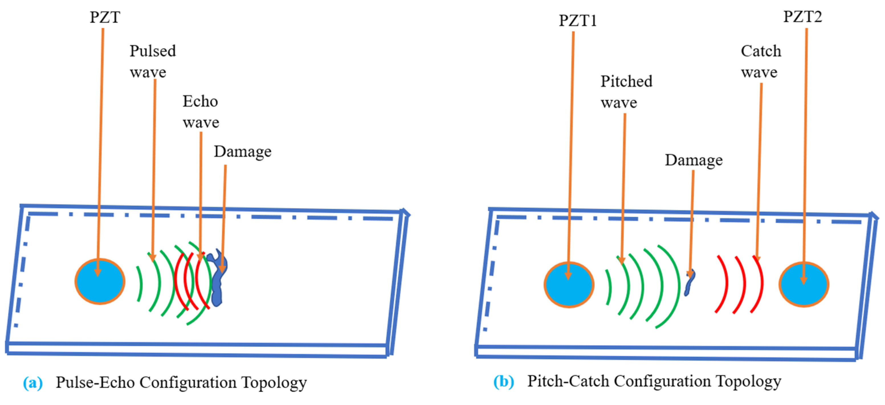
Figure 4.
(a) The implemented damaged plate with bonded PZTs, (b) the calibrated empty damage, and (c) the progressively filled damage.
Figure 4.
(a) The implemented damaged plate with bonded PZTs, (b) the calibrated empty damage, and (c) the progressively filled damage.

Figure 5.
The experimental setup for data acquisition.

Figure 8.
The relative RMS response of the plate under varying temperatures.

Figure 9.
Power spectrum of the captured response signals at different temperatures by PZT2.

Figure 10.
The relative RMS response of the incident wave at varying crack depth.

Figure 11.
The percentage change in the relative RMS as crack depth increases.

Figure 12.
The effect of temperature on 1.5 mm damage depth.

Figure 13.
Temperature effect on 2 mm damage depth.

Figure 14.
Surface plot of the combined influence of damage depth and temperature.
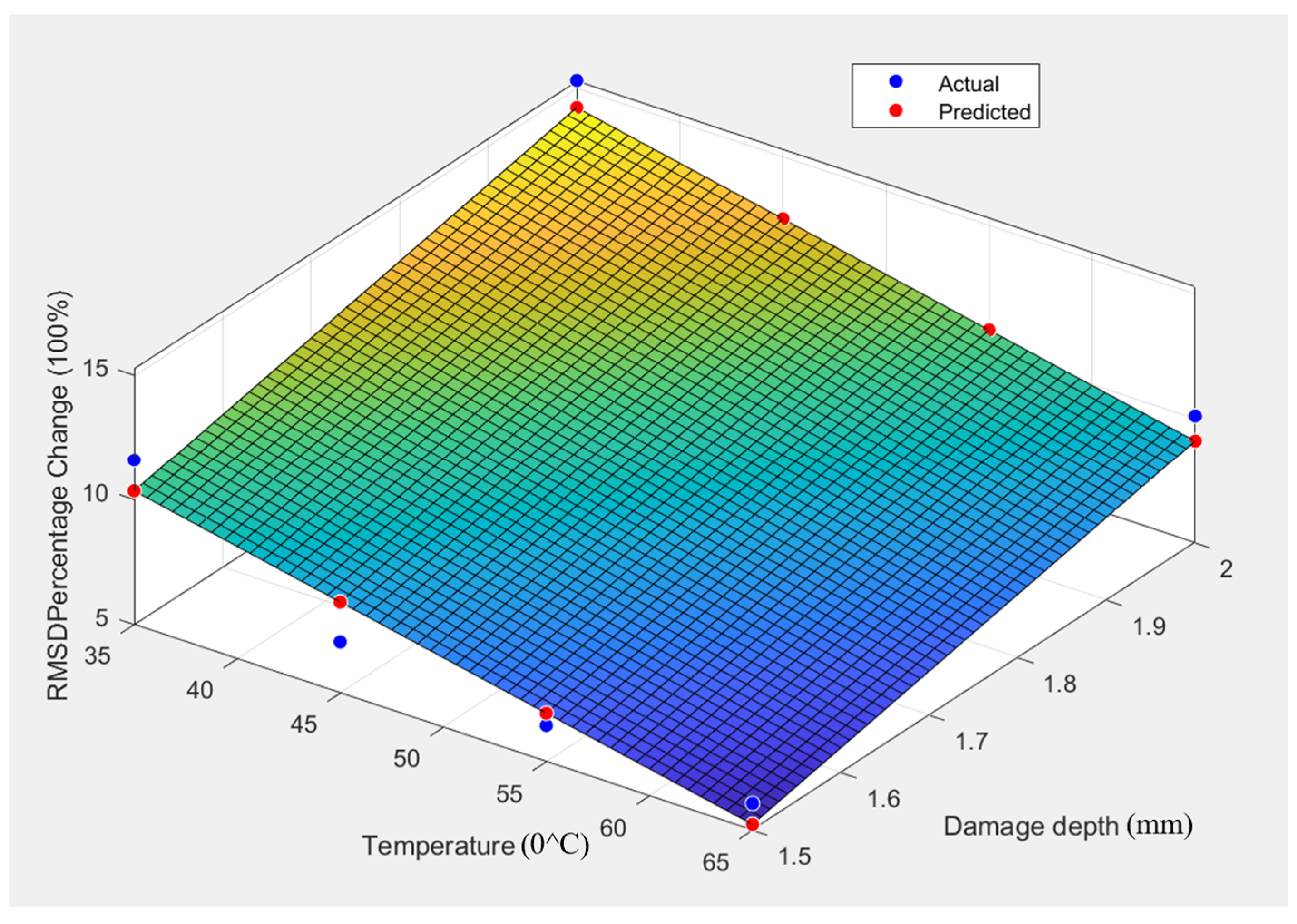
Figure 15.
The effect of debris-filled damage on the guided wave.

Figure 16.
Debris-filled damage-depth factor.

Figure 17.
Surface plot of the combined influence of debris-filled damage and temperature.

Figure 18.
Predictive model response and measured test response.

Table 1.
Mechanical properties of mild carbon steel.
| Material | Young Modulus, E (N/m2) | (kg/m3) | Length, L (mm) | Width, W (mm) | Thickness, Th (mm) | |
|---|---|---|---|---|---|---|
| Mild Carbon steel | 0.289 | 7800 | 500 | 300 | 3 |
Table 2.
The properties of PZT used in the study are PZT-5A.
| Parameter | Unit | Min. Value | Typical Value | Max. Value |
|---|---|---|---|---|
| Diameter of ceramics | mm | 6.80 | 7.00 | 7.20 |
| Thickness of ceramics | μm | 175 | 195 | 215 |
| Curie temperature | Tc | 340 | ||
| Piezoelectric constant | pC/N | 420 | ||
| Elastic compliance | m2/N | |||
| Serial resonance frequency fs | kHz | −5% | 285 | +5% |
Table 4.
Comparing empty and debris-filled DI.
| Crack Depth (mm) | Empty Damage DI | Debris-Filled Damage DI | Debris Factor |
|---|---|---|---|
| 1.00 | 0.408000000 | 0.7058892961 | 1.730120824 |
| 1.50 | 0.367800000 | 0.6449988693 | 1.753667399 |
| 2.00 | 0.114700000 | 0.6519333363 | 5.683812871 |
| 2.50 | 0.085000000 | 0.5202911002 | 6.121071767 |
Table 5.
Comparing the predictive model response with the measured sensor response.
| Debris | Temp. | Predicted Response | Measured Response | Relative Percentage Error |
|---|---|---|---|---|
| 20 | 45 | 0.001400 | 0.001442 | 3.01 |
| 40 | 55 | 0.001507 | 0.001495 | 0.78 |
| 80 | 65 | 0.001709 | 0.001868 | 9.31 |
| 100 | 25 | 0.001758 | 0.001692 | 3.75 |
Disclaimer/Publisher’s Note: The statements, opinions and data contained in all publications are solely those of the individual author(s) and contributor(s) and not of MDPI and/or the editor(s). MDPI and/or the editor(s) disclaim responsibility for any injury to people or property resulting from any ideas, methods, instructions or products referred to in the content. |
© 2024 by the authors. Licensee MDPI, Basel, Switzerland. This article is an open access article distributed under the terms and conditions of the Creative Commons Attribution (CC BY) license (https://creativecommons.org/licenses/by/4.0/).
Share and Cite
MDPI and ACS Style
Olisa, S.C.; Khan, M.A. Confluence Effect of Debris-Filled Damage and Temperature Variations on Guided-Wave Ultrasonic Testing (GWUT). Processes 2024, 12, 957. https://doi.org/10.3390/pr12050957
AMA Style
Olisa SC, Khan MA. Confluence Effect of Debris-Filled Damage and Temperature Variations on Guided-Wave Ultrasonic Testing (GWUT). Processes. 2024; 12(5):957. https://doi.org/10.3390/pr12050957
Chicago/Turabian StyleOlisa, Samuel C., and Muhammad A. Khan. 2024. "Confluence Effect of Debris-Filled Damage and Temperature Variations on Guided-Wave Ultrasonic Testing (GWUT)" Processes 12, no. 5: 957. https://doi.org/10.3390/pr12050957
Note that from the first issue of 2016, this journal uses article numbers instead of page numbers. See further details here.