
Optimized Dynamic Vehicle-to-Vehicle Charging for Increased Profit

Department of Computer Science and Electrical Engineering, University of Maryland, Baltimore County, Baltimore, MD 21250, USA
*
Author to whom correspondence should be addressed.
Energies 2024, 17(10), 2243; https://doi.org/10.3390/en17102243
Submission received: 13 February 2024
/
Revised: 30 April 2024
/
Accepted: 3 May 2024
/
Published: 7 May 2024
(This article belongs to the Section E: Electric Vehicles)
Abstract
:Many challenges have arisen as a result of the rapid growth of the electric vehicles (EVs) market, due to the lack of charging infrastructure capable of handling such a large number of EVs. To alleviate power grid system overloads and reduce the cost of corresponding infrastructure deployments, a direct vehicle-to-vehicle (V2V) energy exchange strategy has become an emerging research topic. In this paper, we formulate the problem of V2V energy charging on a time–space network and develop a dynamic-programming solution methodology for efficiently finding the solution. The algorithm can pair and route the energy supplier (ES) and the requester (ER) in such a way that maximizes the supplier’s profit. Specifically, the ES is incentivized to rendezvous ERs at any encounter nodes in order to dispense the requested energy amount through platooning. Unlike existing V2V charging solutions, our approach involves charging while vehicles are in motion. We validate the effectiveness of our approach in maximizing the profit of the ES and reducing the incurred overhead on the ER in terms of increased trip time, distance, and energy consumption.
1. Introduction
The world has witnessed an improvement in the design of electric vehicles (EVs). EVs have the potential to be a critical technology in the future for mitigating the effects of climate change when compared to internal combustion engine vehicles. The recommendation of the Intergovernmental Panel on Climate Change is to immediately reduce carbon emissions by 45% from 2010 and 100% around 2050 [1]. Thus, automobile manufacturers and policymakers are putting a greater emphasis on EVs, which offer compelling alternatives toward environmental, social, and health-related goals. In the United States, the federal government intends for electric vehicles to account for 50% of new vehicle sales by 2030 [2]. In California alone, an executive order has been issued mandating that, by 2035, all new cars sold be zero-emission [3]. The rapid deployment of EVs could overload the power grids at peak hours, resulting in degrading grid stability, and blackouts. Therefore, new technical and intellectual energy management solutions need to be developed to facilitate the extra loads and continued integration, with over 250 million EVs expected to be on the roads by 2030 [3]. However, the lack of charging infrastructures, the limited range of EVs, and their extremely long battery-charge times pose critical constraints to their widespread adoption. In addition, long-distance trips necessitate careful planning to locate suitable charging stations in order to prevent energy shortages. Luo et al. [4] analyzed the battery capacity and maximum range of several electric vehicles in Table 1. In spite of the fact that maximum ranges are typically greater than 150 km, the information provided by EV sellers is typically derived from laboratory testing. In reality, the actual driving range is impacted by the surrounding environment, such as onboard power electronics, device energy needs, and atmospheric conditions.
The existing charging infrastructure is inadequate to fulfill corresponding high levels of demand. Hence, increasing the number of charging stations throughout the network is a viable approach to promoting the use of EVs. However, building public infrastructure is prohibitively expensive and represents the biggest obstacle to broad use of EVs. Moreover, the increased population of charging stations in urban areas raises concerns regarding the negative impacts of EV charging on the power grid [5]. Employing larger batteries might represent another potential solution to facilitate the wider adoption of EVs. However, oversized batteries provide a number of barriers regarding cost and weight. The cost of an EV’s powertrain is 75% attributable to the battery [6]; thus, deploying a larger battery would substantially increase the overall cost. In addition to the cost concern, large battery packs are cumbersome and occupy a considerable amount of vehicle space, requiring significant power to operate.
Due to the limited battery capacity of EVs and the scarcity of charging stations, vehicle-to-vehicle (V2V) charging has emerged as a promising solution to help address these challenges with minimal infrastructure investment. It can help mitigate the congestion and high load on the grid during peak charging-demand periods. This concept presents the potential for EVs to transfer electric power without directly relying on the utility grid or any external sources of power. It permits EVs to sell and transfer their excess energy to other EVs with an energy demand that is either stationary (e.g., while parking) or dynamic (e.g., while driving). Therefore, vehicle-to-vehicle charging provides EV drivers with more flexible alternatives, helps to reduce EV energy consumption, and allows drivers to earn extra revenue. This can also be leveraged as a business model by operating an EV fleet with surplus energy to serve as the supplier for multiple EVs that are in demand.
As a more versatile and convenient technology for V2V charging, wireless power transfer (WPT) has gained significant interest from both industry and academia. The WPT is categorized as either static wireless charging (SWC) or dynamic wireless charging (DWC). SWC systems transmit power to vehicles in a stationary mode using fixed coils, whereas DWC systems can potentially transfer power to vehicles in motion. Despite the rapid development of SWC over the last decade, the large battery size and the requirement for static charging continue to be drawbacks [7].
Employing DWC systems is a potential solution for boosting the competitiveness of EVs on the market and overcoming charging issues. Consequently, adopting dynamic wireless power transfer (DWPT) systems could offer numerous advantages that promote EVs. One of these advantages is expanding the driving range of automobiles if the battery could be continuously charged while the vehicle is in motion, hence extending the traveled distance. Moreover, DWPT avoids stoppage delay since the vehicle continues to travel during charging.
The problem, which is modeled as a vehicle routing problem, seeks to optimally route ES to approach and serve ERs to fulfill their energy demands. The main objective is to maximize the profit of the supplier, while considering battery degradation and the overhead cost. The complexity of the problem arises from non-stationary consumers (ERs) and service supply, which makes monitoring and synchronizing the movement of ES and ER spatiotemporally challenging. In this study, we introduce an integer programming (IP) formulation based on the concept of a time–space network. We also propose a solution methodology that comprises constructing a time–space expanded network and dynamic-programming solution methodology to find the optimal routes on this expanded network. We posit the existence of a cloud server with the capability to efficiently disseminate pertinent information and execute the requisite algorithms, serving as a centralized hub for coordinating the dynamic exchange of energy among ES and ERs.
The rest of this paper proceeds as follows: Section 2 presents a literature review. In Section 3, we present a clear description and a formal mathematical formulation of the problem. Section 4 shows the solution methodology. Section 5 presents the validation and results. Section 6 concludes our work and proposes further research directions.
2. Literature Review
Infrastructure-supported EV Charging: Fixed-point charging of EVs refers to the use of charging infrastructure to replenish the battery supply. Such a methodology, which sometimes is called stationary charging, is the most prevalent and can be categorized into: (i) power-line charging stations [8,9], (ii) battery-swap depots [10,11], and wireless charging lanes [12,13]. However, fixed-point charging remains a major concern for many EV drivers in urban areas due to the insufficient power-line charging stations required to meet demand. Furthermore, EVs require a considerable amount of time to recharge; hence, waiting times at public power-line charging stations can easily become excessive, especially during peak traffic periods. Wireless charging lanes and battery swapping are two potential alternatives that are being considered to address the scarcity of power-line charging stations. However, the installation of wireless charging lanes is incredibly costly, ranging from approximately $1.1M to $2.8M per kilometer [12,14,15]. A substantial portion of these costs is attributable to the integration of charging pads into road construction. Moreover, due to the isolated nature of implementation, charging pads will be inaccessible for future maintenance and improvement after installation. For battery swapping, the construction costs might be lower than those for charging lanes, yet there are some obstacles that make this method both technically and economically inefficient. The requirements for standardization are stringent, as the batteries are frequently transferred among vehicles of varying makes and models. In addition, the lack of clarity regarding ownership of the battery will increase safety and user concerns and present warranty and liability issues [16]. Even though the battery-swapping revival in China it is not likely to gain significant traction in other developed countries like the United States [17]. Several automobile manufacturers, such as Tesla, have introduced battery-swapping stations. However, the development of this concept has been plagued due to: (i) the lack of consumer acceptability caused by concerns about not owning the battery, and (ii) the potential tampering with their original battery [18,19].
Work on fixed-point charging can be classified based on what aspect is being optimized into: (i) where to deploy the service, e.g., the position of the charging station, and (ii) when an EV is to be charged. Service placement optimization is in essence an asset planning problem where reachability and coverage are the popular metrics that published studies consider [20,21]. The objective is to make sure that an EV can replenish its energy supply without getting stuck on any road segment. Meanwhile, scheduling EV charging is typically modeled as a vehicle routing problem (VRP). The limited driving range of EVs could necessitate battery recharging in the middle of a trip and hence the location of charging services should be factored in the route selection [22]. Several studies have considered these factors to model the behavior of EVs and to determine the optimal location of charging stations [23,24]. Sun et al. [25] have proposed a placement optimization model for charging stations based on travel patterns of urban residents to maximize charging-demand satisfaction. Their model comprises two parts, one for short-distance commuters with slow charging facilities and another for long-distance journeys with fast charging technology. Zhang et al. [26] have utilized an ant colony optimization algorithm and adaptive large neighborhood search to solve the placement problem with an objective to reduce energy overhead in reaching the charging station relative to the shortest route. The placement algorithm of Guo et al. [27] considers the user’s distance anxiety and satisfaction as a metric, where anxiety reflects the user’s risk tolerance and the impact of battery depletion during a trip. However, these placement algorithms assume that an EV will visit a charging station for energy replenishment, which is both inconvenient and time-consuming as noted earlier.
V2V Charging: V2V charging represents an innovative paradigm shift in the realm of EVs and sustainable transportation that can play a significant role in addressing the shortage of charging stations. This technology leverages the inherent capabilities of EVs as mobile energy storage units, enabling them to function as both consumers and providers of electricity. In a V2V charging scenario, an EV with surplus energy can transfer power to another vehicle in need, fostering a dynamic energy-distribution network. Several solutions were proposed concerning the concept of energy exchange between EVs at designated hubs that are less costly to construct than a charging station because grid connectivity is not necessary [28,29,30]. The idea of distributing trucks to charge EVs has been proposed in the literature [31,32]. The trucks are initially charged at a depot, and after serving EVs at a designated location (i.e., a parking lot), they should return to the depot before becoming completely depleted. A robot-based distribution has been also developed in some studies [33,34], where a robot transports a mobile energy-storage device in order to charge EVs while they are parked without human intervention. However, these V2V charge-sharing solutions require that both the requesting and supplying vehicles remain stationary during battery charging and hence does not mitigate the latency concern of fixed-point charging options.
Dynamic charging has emerged as an effective methodology that represents a transformative advancement in EV technology, introducing a dynamic and flexible approach to charging on the go. Unlike traditional static charging stations, mobile V2V enables EVs to transfer power between each other while in motion. This concept not only enhances the convenience of electric mobility but also addresses concerns related to limited charging infrastructure. Specifically, employing mobile V2V charging services is deemed to be an innovative solution that can tackle the challenges impeding the widespread adoption of EVs. Existing studies have demonstrated that mobile V2V charging can be achieved by either wireless power transfer (WPT) [35,36] or converter cable assembly charging [37,38]. While the latter requires physical connection to transfer the energy between EVs, WPT technology utilizes electromagnetic fields without the need for physical cables, offering a seamless and convenient charging experience. The advancement of mobile V2V charging owes much to the precision vehicle coordination facilitated by Connected and Automated Vehicle (CAV) technology, such as Adaptive Cruise Control (ACC) and Cooperative Adaptive Cruise Control (CACC), allowing for close alignment and small inter-vehicle gaps. CAV technology empowers vehicles to operate with minimal spacing, forming and maintaining platoons of interconnected vehicles capable of mutual power supply, thereby reducing the likelihood of accidents or collisions stemming from the close proximity [39,40,41].
A number of studies have already investigated the prospective implementation of mobile V2V WPT strategies to promote their utilization. For instance, Kosmanos et al. [42] and Moschoyiannis et al. [43] have proposed wireless mobile charging systems where city buses supply energy to EVs through platooning. When the buses complete their round trips, they will return to the fixed charging station where the batteries will be completely charged or replaced. However, the predefined routes and schedules of the buses limit the coverage and the flexibility of the service. Liu et al. [44] present a platoon-based charging, in which EVs line up behind a charger where an EV may have to pursue a detour to join a platoon. They examined the optimal assignment problem between EVs and charging platoons and modelled it into a dynamic weight bipartite matching. Nevertheless, for platoons with more than two vehicles, it is known that the gains for the trailing vehicles are less than those for the leading vehicles. Recent studies [35,45] have introduced a peer-to-peer charging methodology aimed at facilitating energy exchange among multiple EVs, encompassing both energy suppliers and energy requesters. This approach offers operational advantages, including the reduction of management costs associated with provider fleets. The work in [35] presents an in-motion charging platform where EVs recharge in close proximity, guided by a cloud-based control system for coordination. The primary objective is to optimize the number of served requests and the energy efficiency while minimizing infrastructure investment requirements. Meanwhile, the work in [45] explores fleet-management strategies for energy providers dispatched to fulfill EV energy demands while vehicles are in motion. The objective is to minimize the number of dispatched vehicles, thereby reducing the traffic generated by the supplier fleet. To the best of our knowledge, no prior work has considered the routing problem of a mobile energy supplier for maximum profit.
Vehicle Routing Optimization: From an optimization perspective, this study showcases a strong correlation with two well-established Vehicle Routing Problem (VRP) models that are widely considered in the existing literature: the Dial-a-Ride-Problem (DARP) and the routing with flexible targets. DARP focuses on optimizing the routes and schedules of a fleet of vehicles catering to dynamic on-demand passenger requests; in the context of dynamic V2V charging scenarios, these requests reflect electric vehicles’ interaction to exchange energy in real time. Yet, the dynamic V2V charging problem introduces a higher level of complexity that stems from its inclusion of non-stationary customers and the delivery of energy services, which necessitates synchronization of both spatial and temporal movements of energy suppliers and requesters. In other words, unlike the DARP, where pick-up and drop-off locations are predetermined, the dynamic V2V charging problem requires determining when and where a supplier can meet, platoon, and detach from a requester, thus adding intricacy to the formulation of the problem.
Similarly, the routing with flexible targets extends traditional VRP formulations by considering mobile destinations, aligning with the essence of V2V charging where vehicles serve as both energy providers and recipients. A primary variant of routing with flexible targets encompasses scenarios with moving targets [46,47] where vehicles are tasked with intercepting non-stationary targets that move dynamically in the Euclidean plane. These targets could represent mobile customers, changing delivery locations, or dynamic service requests. Another variant relates to the VRP with roaming targets [48]. This scenario encompasses adaptable deliveries within small-package logistics systems, wherein each customer may be serviced at various locations (e.g., work or home) and at different times throughout the day. Yet each customer is assumed to travel on a straight path at a consistent speed [45]. In our work, each requester follows its designated route, and the product being delivered is electricity, which can be transferred through platooning.
3. Routing Problem Modeling
Time plays a crucial role in the model in many vehicle routing and scheduling problems. However, the conventional modeling approach to routing and scheduling problems in the majority of the literature typically includes time as a variable in the model and employs a large number of big-M constraints to capture the logical relationships. Adding continuous variables to an integer program and utilizing big-M constraints often results in voiding the linear relaxation of the model, which typically increases the complexity. To more effectively manage time, new modeling techniques, such as continuous-time modeling and time–space network modeling have been applied to these problems. In this study, we formulate the problem with the help of a time–space network, which allows embedding the scheduling aspect of our problem in the network. The notation will be defined as needed; a reader can refer to Appendix A for a quick reference.
3.1. Construction of the Time–Space Network
Assume that the road network is given as a directed graph , where denotes a set of nodes and is the set of arcs. To model the problem as a time–space network (TSN), we expand so that each node represents a location in time, and each arc represents a transition from one location to another that takes a certain time duration. Let denotes this time–space network, where is the set of nodes and is a set of arcs. A node is represented by a pair of time and space (location), , where is the time, and is the location in the road network. The set contains several types of arcs, as described in detail below. An arc in is a pair where , and . However, to simplify the notation, we use , or or when we do not explicitly need to consider the time attribute. If we do so, we may refer to the nodes’ attributes with to refer to its time, and to refer to its location.
We discretize time based on a certain epoch and reflect the temporal order of requesters. First, let denote the set of points in time when an ER can start its trip, where and are the earliest departure and latest arrival times, respectively. In some cases, flexibility exists with respect to the ER’s schedules. Let denote the total travel time for the given route. Accordingly, is the total travel time for the route of the ER . If , and the schedule of the ER is deemed to be flexible, meaning that this ER can adjust the travel schedule to facilitate synchronization with the ES. Therefore, the ER can choose when it starts its trip, but will not pause traveling along the way. Given , we can derive the set of possible departure times at each location (node in N) along the route. Let denote the set of possible start times at the k-th node of the route . For example, assume ER drives route , where its earliest departure is time 12 pm and its latest arrival is time 4 pm. Driving from node to takes one hour, and driving from to takes two hours. Therefore, the total driving time is only three hours and the time window in which the ER starts its route is from 12 pm to 1 pm. Assume that we discretize this interval and receive Accordingly, we have and .
Supplying arcs: A supplying arc is a road segment on which the ES is platooning with a requester. We can simply represent a supplying arc for some and a segment on its route as , where , and . If the energy provider traverses multiple consecutive supplying arcs, the tail of the first arc can be considered as a rendezvous node since it is where the ES platoons with the ER. Let denote the set of supplying arcs; we define the following three related sets:
- signifies the set of supplying arcs associated with an ER , where ;
- reflects the set of supplying arcs for a requester with a tail node . Specifically, where is the start time at the tail node and is the arrival time at the head node;
- represents the set of supplying arcs of ER with departure time It is defined as , with and as previously defined. Again .
The energy needed for traversing an arc in is (), which reflects the emitted energy to the requester and the energy overhead of traveling the segment , where denote the energy that can be charged on the road segment , which is the product of transmission power and the travel time (). The cost needed for traversing an arc is where and are the sell and purchase prices per unit of energy, and is the battery degradation cost. Referring to [49], the battery degradation is impacted by a number of factors including the battery replacement cost (), residual battery at the end of life, which is typically defined as 80%, battery degradation factor (), battery capacity (), and charging/discharging rate. Therefore, the degradation cost is given as Due to the fact that some energy is lost during transmission, we actually need units for each supplied unit, where is the charging factor.
Deadheading arcs: A deadheading arc represents a road segment that the supplier travels without a client, and is represented as , where and take on values depending on the supplying arcs and and . When starting the trip or after having traversed a supplying arc, the ES may choose to deadhead to any location and, if necessary, traversing multiple segments of the road network. If the ES deadheads, we assume that it always chooses the fastest path, i.e., least travel delay. To capture the potential of deadheading in the time–space network, a deadheading arc is added from the current node to any location. For example, assume that the ES deadheads from location to location starting at some point in time and that there is no direct link from to in the road network, that is, they are not adjacent in the road network . The supplier then chooses the shortest path and traverses a single deadheading arc in the time-space network, and the time needed is the travel time of shortest path from to . Let denote the set of deadheading arcs, and and denote the total travel time and total energy consumption of the shortest (least delay) path from node to node , respectively. Hence, the cost for traversing a deadheading arc is which we denote as . Let denotes the start point of the ES’ trip. The set of deadheading arcs is:
That is, we create a deadheading arc from the origin and from each node where a supplying arc ends to every other location in the road network. Note that we may have two arcs between the same two locations—one supplying arc and one deadheading arc. It may improve the total profit to traverse the deadheading arc instead of the supplying arc in order to use the saved energy for a more profitable opportunity later on.
Waiting arcs: The purpose of the waiting arcs is to allow the supplier to wait at its current location until the next opportunity (request) arises. Therefore, the tail and head nodes of a waiting arc are associated with the same location of the road network, and we can represent a waiting arc as where < and . In the following, we use to denote the ordered sequence of nodes associated with location with an increasing time. To obtain for each , we first create the set We then eliminate potential duplicates in , and sort it according to time. Now, we connect consecutive nodes in by creating a waiting arc. For instance, assuming that , we create two waiting arcs and . We do not need another waiting arc like Let denote the resulting set of waiting arcs. Let denote the cost of waiting one time unit. The energy consumption of a waiting arc is zero.
Illustrative Example: We illustrate the time–space network with a simple example as shown in Figure 1. The road network consists of three nodes and arcs . The driving time is one hour from A to B and back, two hours from B to C and back, and one hour from C to A and back (left side of Figure 1). The ES starts at node A and ends at node C. There is one ER with traveling . The total driving time is three hours. The earliest departure time of requester #1 (the only ER in this example) is and the latest arrival time is ; consequently, the latest departure time is 13, given the total driving time With we have and Hence, we can choose among two different departure times for the requester. If the requester departs at 12, we can charge along the link (A, B) starting at time 12 and/or charge along the link (B, C) starting at time 13. If the ER departs at time 13, we can charge along the link (A, B) starting at time 13 and/or charge along the link (B, C) starting at time 14. In other words, there are four supplying arcs, as depicted in Figure 1. The network is expanded by inserting the ES’s source node (0, A) and by adding waiting and deadheading arcs, as shown in Figure 1. Now, we need to find the most profitable route that starts at node A and ends at node C.
Multi-graph: First, during the creation of the time–space network, it can happen that two nodes with the exact same coordinates would be created. For instance, there might be two supplying arcs from different requesters that terminate at the exact same time and location. Therefore, when building the time–space network iteratively, we make sure to not create duplicate nodes, and instead reuse an existing node, should one with identical time and space values already exist. Second, there can be multiple arcs between the same two nodes, that is, the time–space network is a multi-graph. For instance, supplying arcs from different requesters can have the same tail and head nodes, or a supplying arc and a deadheading arc might coincide. In the latter case, it may be beneficial to use the deadheading arcs in order to save the energy for a later request that generates more profit. Therefore, the tail and head nodes are not sufficient to identify an arc. To identify an arc, we must know its type (supplying, deadheading, or waiting), and, if it is a supplying arc, we also need to know the requester and the index of the tail node. Another consequence of the time–space network being a multi-graph is that we must use an incident list representation instead of an adjacency list representation. Let denote the set of arcs incident to node where is the tail node of these arcs and let denote the set of arcs incident to node where is the head node.
3.2. Time–Space Network Formulation
With the time–space network, we can also formulate the optimization model as an integer program (IP) with binary decision variables for , which is equal to one, if the supplier traverses arc , and zero otherwise. Assume that and . The energy needed to traverse arc is defined as:
The cost of traverse arc is defined as:
Additionally, the binary variable is equal to one, if ER receives energy and starts its tour at time , and zero otherwise. The problem can be formulated as follows:
Subject to
The objective function (3) minimizes the total costs comprising the cost for deadheading, waiting, and the revenue for supplying energy. Constraints (4) ensure that the supplier indeed departs and make a trip (leave the initial position). Constraints (5) are the flow balance that make sure that the out-degree of each node is at most as large as the in-degree; they fundamentally ensure continuity of the formed path. Constraints (6) ensure that the tour terminates at the destination node. Constraints (7) and (8) make sure the energy capacities of the ES and an ER are not violated, respectively. Constraints (9) set force the indicator variables to one if an ER receives energy via a supplying arc that is associated with the corresponding travel start time. Constraints (10) ensure that one specific travel start time is selected for each ER that receives energy. Constraints (11) make sure that if an ER receives energy and starts its route at a certain time, it will receive at least the required minimum quantity of energy. Finally, Constraints (12) and (13) define the variable domains.
4. Optimization Formulation and Solution
4.1. Shortest-Path Problem
With the time–space network, we can solve the problem by finding the least-cost path from the source to the destination node. However, there are several additional constraints that must be considered. First, apart from the costs, the ES’s energy is a second resource, and we cannot exceed the ES’s energy capacity (See Constraints (14)).
Let be a path from the source to the destination of the TSN, and let
is simply a variable to capture whether a supplying arc is part in the solution of the routing problem (part of the optimal path); if so the requester “r” is noted. For .
The energy capacity is limited by
Ignoring all other further constraints, the problem is a Shortest-Path Problem with Resource Constraints (SPPRC). We are considering the two-resource version of SPPRC, which is known as the Shortest-Path Problem with Time Windows (SPPTW) [50]. In our case, the additional resource is energy instead of time, and the time window of each node (typically denoted as []) is an energy window equal to for all nodes. This problem is also called the Shortest-Path Problem with Additional Constraints (SPPAC) [51]. Furthermore, since the network is acyclic, the supplier can visit each node at most once. Hence, feasible paths are elementary, and due to this property, this problem is sometimes called the elementary SPPRC [52].
In addition to ES’s energy capacity, there are some restrictions that cannot be handled by simple resource windows or by removing some arcs or nodes from the time–space network. A path from the source to the destination that does not exceed the ES’s energy capacity is feasible if the following structural constraints hold.
- The path can only contain supplying arcs of a given requester that belong to the same departure time:This ensures that we select only one departure time for each ER that receives energy.
- If the path contains supplying arcs associated with a given ER, this set of arcs must be a path:i.e., the set of arcs on the left side is a path. This ensures that the charging process of any ER cannot be interrupted.
- The path cannot contain supplying arcs that overcharge the ER battery:This ensures that the energy balance of each ER does not exceed its battery capacity at any node along its route.
- If the path contains one or more supplying arcs of a given ER, there must be sufficient supplying arcs in the path so that the ER receives at least as much as energy as the minimum threshold.Particularly, we do not need any synchronization constraints since: (i) the ERs start their routes within the allowed time windows by the definition of the supplying arcs, and (ii) a path in the TSN already defines the timing of the ES.
4.2. Dynamic-Programming Solution Methodology
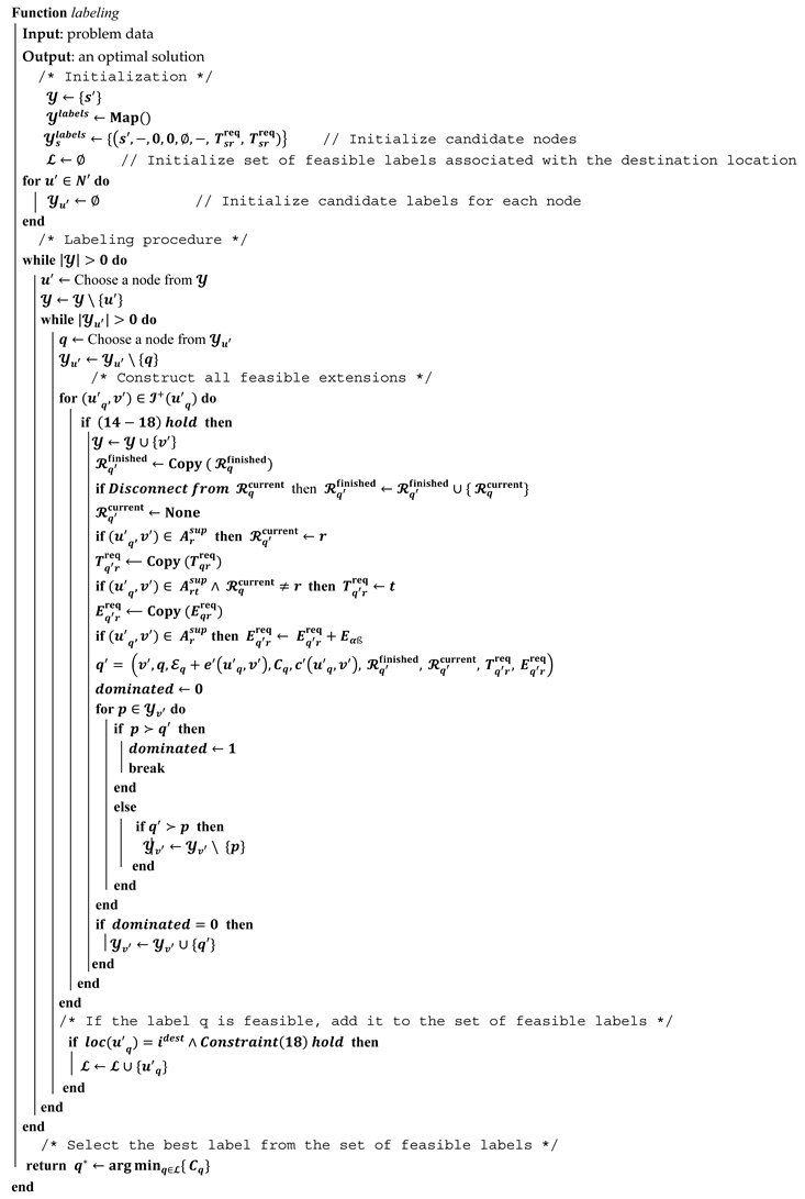
By definition, the time–space network is a directed acyclic multi-graph with arbitrary costs. It is a multi-graph because it can have multiple arcs with identical tail and head nodes (e.g., when multiple requests from different requesters coincide). Traversing deadheading arcs incurs a cost while traversing supplying arcs generates revenue. The objective is to identify the paths with the minimum cost that connect a source node to the destination node, while ensuring that the total consumption of resources along the path falls within specified lower and upper bounds. Dynamic-programming-based labeling is widely recognized as one of the most efficient frameworks for resolving multiple variants of the SPPRC. Therefore, we propose a node labeling algorithm for solving our optimization problem. The algorithm is also similar to the branch and cut methods that involve pruning the pool of solutions to be explored based on dominance criteria and bounds derived from partial solutions that have been already discovered; therefore, obtaining the optimal solution is possible before labeling all nodes.
The network is stored as an incidence list, , where denotes the set of incident arcs departing from node . Recall that each node comprises time and location. We start with a trivial path containing only the source node (ES starting point), , and extend from there to build new paths until we reach the destination. Each path is represented by a label that comprises all the necessary data to determine the path (via backtracking) and to apply the dominance criterion described below. In particular, label comprises the following elements.
- The node is associated with (commonly called the resident node of the path).
- A reference to the predecessor label . Chaining labels to their predecessors in that way is an efficient way to keep track of the paths [53].
- The total consumed energy of the ES’s battery up to the current node, .
- The total costs up to the current node, .
- The set of ERs that have been served, , where only ERs from which the ES has disconnected already are included.
- If the ES is currently connected to an ER, then the ER identity is stored in, .
- is a mapping stores the departure time of all ERs. If an ER has not received any energy yet, it takes on an arbitrary value.
- is a mapping that stores the total received energy of all ERs. If an ER has not received any energy yet, it takes on the value zero.
In the dynamic-programming algorithm, we maintain a set of candidate nodes denoted as , and for each candidate node , we maintain a set of candidate labels denoted as . Initially, we set , and where, is not relevant and, for all . During the procedure, we iteratively choose a node from and remove it from . We then iteratively pick a label associated with node from the set , remove it from so that it is not considered further. We then extend the label’s path along all outgoing arcs, if extending the path with the corresponding arc is feasible. Extending the path of label via arc is feasible if the following constraints hold.
Constraint (14) ensures that the total energy consumption does not exceed the capacity of the ES. Constraint (15) prevents that charging from being interrupted. Constraint (16) is to allow only one departure time to be selected for each ER. We already know from the previous constraint that the considered ER is not among the ones that were served in the past. Hence, if the ER is not currently being served, it is selected for the first time, and the departure time can be chosen from the set . Otherwise, if the ER is currently being served, its departure time must match what has already been set. Constraint (17) protects the battery of an ER from being overcharged. Constraints (18) ensures that we can only disconnect from the ER if we have supplied the minimum required quantity of energy. If we have not yet supplied enough energy and none of the incident arcs allows supplying additional energy, then the current label is infeasible.
If all these conditions are met, the algorithm creates a new label where are set as follows.
- The set records fulfilled requests, which can occur in two scenarios: (i) if the current ER remains connected, implying , or (ii) if the demand of the current ER is fulfilled, resulting in the ER no longer being in platooning with the ES, i.e., .
- The set maintains potential start times for an ER which can vary based on two scenarios: (i) the ER has begun charging and the new departure time for this specific ER is added, i.e., , where , or (ii) the ER has not commenced charging, hence there are no changes in start times, i.e., .
- represents the total energy received from supplying arcs. If a supplying arc is traversed, is to be augmented with the energy received by the ER that is being currently served, i.e., . Otherwise, no change is made, i.e., .
Then, we add the new label to the set of labels associated with the destination node , unless there is an existing label that dominates the new one. Additionally, existing labels dominated by the new label are discarded. The domination criterion is described below. We also make sure that labels associated with the destination node are not discarded. Once the list of candidate nodes is empty, we pick the label with the lowest costs from the labels associated with the destination node, and backtrack via the predecessor references to obtain the optimal route. A pseudo code summary of the steps can be found in Appendix B.
Domination criterion: If two labels and are associated with the same node, it is feasible for to be at least as effective as . For such an instance, we state that dominates , denoted as , and can therefore be discarded without impacting optimality because any route incorporating is no better than one where is replaced with . More precisely, holds true if the following conditions are satisfied:
Condition (19) ensures that both labels must be associated with the same node. Conditions (20) and (21) state that the dominance relation does not hold, if the total used energy and the total cost are greater, respectively. Condition (22) states that a label that has an ER in the finished list cannot dominate another label. Per Condition (23), dominance is only possible if either both labels do not have a current ER, or both labels have the same current ER with identical starting times.
5. Numerical Study
5.1. Experiment Setting
We have conducted a number of numerical experiments to analyze the efficiency of the proposed approaches. The experiments consider the road network of the city of Sioux Falls and assess performance under varying ER count. The ER’s battery capacity is assumed to be in the range of 45 kWh to 95 kWh with consumption rate of 0.19 to 0.24 kWh/km. We assume that the supplier has a battery size of 95 kWh, which reflects the battery of Tesla Model S, and is permitted to carry multiple batteries as part of its business operations. We further assume that the driving range anxiety is relaxed, allowing requesters to depart their workplaces or residences without fully charged vehicles. We consider a power-transfer rate of 50 kW, and 95% transfer efficiency. The energy prices are obtained from the U.S. Energy Information Administration (EIA), where is based on the residential electricity prices [8–10 ¢/kWh], and is set to [40–60 ¢/kWh]. This pricing strategy allows the supplier to capitalize on favorable market conditions, such as purchasing energy at lower rates and selling it at higher prices, particularly during periods of increased demand, e.g., during rush hours. The battery degradation factor and the battery replacement cost are set to 0.0027% and 150 $/kWh, respectively [49].
An ER trip is randomly selected from a public dataset of 360,600 trips [54]. Each entry in the dataset specifies the origin, destination, start time and arrival time. Time is discretized into 5 min’ intervals. We conduct the experiments under two scenarios: (i) V2V, and (ii) charging stations (CSs) only. For more fair comparison with dynamic charging, we only consider level 3 fast-charging stations. The distribution of charging stations in the area is shown in Figure 2, where the locations are based on the PlugShare network [55]. We assume that there is no queue in the charging stations, and ERs may not necessarily fully charge their batteries; such assumption is to align the operation with the dynamic V2V charging. All numerical experiments are performed on a machine with 2.2 GHz Intel Core i7 CPU, four cores, and 16 GB of RAM. For each simulation setting, we average the performance over 10 runs.
5.2. Travel Time and Distance
We first compare the average travel time and the average vehicle-kilometer traveled (VKT) by all vehicles, using the aforementioned scenarios. The results depicted in Figure 3a indicate that dynamic V2V charging can effectively decrease the average VKT of ERs from 13 km to 9.2 km. Figure 3b shows that the average travel time when using CS for charging is around 19.2 min; such a time is reduced to around 10.8 min when platooning is pursued. Hence, our approach saves about 40% of ER travel time. Such a reduction is due to the elimination of detours to access charging stations and the eradication of delay while charging.
5.3. Energy and Charging Time
We also compare the energy-consumption rate, the energy supplied to ERs, and the energy loss during transmission for both scenarios. As seen in Table 2, our approach has resulted in a decrease of 15% in the rate of ER energy consumption when compared to the conventional CS-based charging. The decrease in energy consumption is mainly due to the elimination of unnecessary diversions to access fixed charging stations. It is also notable that the energy loss by the supplier during power transmission has obviously a negligible effect when compared to the supplied energy. The loss is attributed to the wireless power transmission that occurs throughout the platoon-based charging process. Meanwhile, the average charging time at CS is longer even without considering any queuing delay. Our approach achieves a major reduction in charging latency; in fact, our approach can be viewed as a means to offload charging stations and minimize their queuing delay in settings where demand is too high for the available ES to handle.
5.4. Profit and Overhead
Figure 4 reports the total ES profit from serving a varying number of ERs, and the total cost of traveling and/or supplying ERs. We can notice that both total profit and overhead costs grow with the increasing number of requesters. Nevertheless, the ES constituently makes profit as the where the revenue always exceeds the overhead.
5.4.1. Comparison with a Baseline Approach
We further validate the effectiveness of our approach with a greedy one as a baseline. We use two different criteria for selecting the next ER based on: (i) the closest rendezvous point (CRP), and (ii) the highest energy demand (HED). In the context of CRP, the ES primarily seeks to minimize overhead costs, whereas HED strives to maximize revenue. Figure 5 and Figure 6 show the average profit and the average overhead costs comparison between our approach and the two greedy heuristics, namely, CRP and HED. As depicted in Figure 5, our approach slightly outperforms HED in terms of profit. However, as seen in Figure 6 and Figure 7, our approach achieves an 11% and 15% reduction in the average travel overhead and tour time in comparison to HED, respectively. Table 3 indicates that half of the tour time in HED is dedicated to deadheading, implying that the ES requires more energy and time compared to other approaches. Consequently, these two figures show that the ES in our approach has a shorter tour and lower travel costs, resulting in a significant reduction in labor expenses, which is not explicitly captured in our simulation. This also has a positive impact on other costs such as wear-out (mileage) and vehicle insurance. On the other hand, CRP outperforms both approaches in terms of overhead cost but majorly lags behind in terms of generated profit. Such performance can be ascribed to the ES’s pursuit of distance optimization, which resulted in lower costs and time but also diminished profitability.
5.4.2. Waiting-Cost Analysis
We have also examined the effect of waiting time (cost) on the profit and overhead cost considering different values of the waiting-cost factor (0.001, 0.01, 0.1). The overhead here involves traveling costs, battery degradation costs when supplying ERs, and waiting costs; the latter is what is being varied across experiments. As seen in Figure 8 and Figure 9, the profit and overhead grow as the number of requesters increases. However, there has been a corresponding decline in profit and a leap in overhead for all the considered values of the waiting factor. A larger waiting factors causes notable performance decline, where the profit and overhead for a waiting actor of 0.1 causes about a 50% drop in profit, and a 24% increase in overhead in comparison to a setting of 0.01. The observed discrepancy can be attributed to the significant costs associated with waiting time, which hinder the supplier’s ability to fulfill numerous requests.
5.5. Computational Complexity Comparison
We compare the performance of our algorithm with an existing open-source solver, CBC, and a heuristic greedy algorithm in terms of the solution time and the objective function value. For each instance, we conducted 10 cases and reported the results as the average of 10 runs in Table 4. As seen in Table 4, the DP algorithm has better performance than the CBC solver in terms of computing time for all instances. While the CBC solver and DP algorithm provide optimized values for the objective function across all instances, the greedy strategy yields somewhat varied solutions for each instance. Although the greedy algorithm converges faster than both approaches, the resulting solution is significantly worse in terms of revenues, i.e., it deviates significantly from optimal. We also observe that the performance of the greedy heuristic seems to deteriorate with the increasing number of requesters. This is mainly because the greedy heuristic does not take advantage of the large number of requests and prioritizes minimizing travel overheads over maximizing profitability.
6. Conclusions
Dynamic EV charging pursues platooning to transfer energy while a vehicle is on move. Such a charging method motivates a business model where a supplier makes tours to sell energy to requesters, thereby fostering entrepreneurship opportunities and stimulating economic growth in the electric vehicle charging sector. This paper has studied the problem of maximizing the ES profit without imposing detours on ERs. A novel approach is proposed to find the ES travel route that achieves such an objective by serving multiple ERs while minimizing the travel overhead by 40%. We formulate such a routing problem as an integer-programming optimization and develop a dynamic-programming solution methodology. The efficiency of our approach is accessed by numerical experiments using the road network of the city of Sioux Falls. The results show that our approach consistently boosts the supplier’s profit under varying requester counts, and outperforms the greedy approach by achieving an 11% and 15% reduction in the average travel overhead and tour time, respectively. This highlights the effectiveness and efficiency of our proposed methodology in optimizing energy-delivery routes for electric vehicles, ultimately leading to improved profitability for energy suppliers.
Moreover, our approach enables savings of 30% and 44% for ERs in terms of travel distance and charging time compared to the use of stationary charging facilities, respectively. In addition, our approach yields a significant decrease of 15% in the rate of ER energy consumption compared to conventional CS-based charging methods due to the elimination of unnecessary diversions required to access fixed charging stations. We also conducted a comparative analysis of our algorithm with two other methods: an open-source solver, a CBC, and a heuristic greedy algorithm. The results indicate that our DP algorithm outperforms the CBC solver in terms of computing time, and it consistently delivers optimized values for the objective function across all instances, highlighting its superior performance compared to the greedy one.
In future work, we plan to consider the problem of maximizing the profit of multiple supplies by optimal ER-to-ES assignments and factoring in non-constant pricing strategies. This entails exploring scenarios where pricing strategies are not constant but vary over time based on factors such as demand fluctuations and energy market dynamics. By addressing these complexities, we seek to develop more robust and adaptable models that can effectively optimize profit margins for multiple suppliers operating within the context of mobile energy-delivery services.
Author Contributions
S.A.: Investigation, Conceptualization, Methodology, Writing—Original draft, Formal analysis, Software, Validation. M.Y.: Conceptualization, Methodology, Formal analysis, Writing—review & editing, Supervision. All authors have read and agreed to the published version of the manuscript.
Funding
This research received no external funding.
Data Availability Statement
The data presented in this study are available on request from the corresponding author. The data are not publicity available due to privacy or ethical restrictions.
Conflicts of Interest
The authors declare that they have no known competing financial interests or personal relationships that could have appeared to influence the work reported in this paper.
Appendix A. Table of Notations

Table A1.
Parameters and variables.
| Symbol | Description |
|---|---|
| Set of nodes | |
| Set of arcs | |
| Set of ERs | |
| Set of nodes of the time-space network | |
| Set of arcs of the time-space network, where | |
| Set of supplying arcs of the time-space network | |
| Set of deadheading arcs of the time-space network | |
| Set of waiting arcs of the time-space network | |
| Set pf supplying arcs associated with ER and the index of the tail node, | |
| Set of supplying arcs associated with ER and departure time | |
| Time of node in the time-space network | |
| Location of node in the time-space network | |
| Length of the route of ER (i.e., number of arcs) | |
| Route of ER (along of which charging can take place) | |
| Energy consumption when traversing arc | |
| Energy consumption when traversing arc | |
| Total energy consumption of a shortest path (in terms of travel time) from node to node | |
| Travel time for traversing arc | |
| Total travel time of a shortest path (in terms of travel time) from node to node | |
| Total travel time for the route | |
| Energy transfer if platooning is performed on arc | |
| Energy transfer if platooning is performed over the link sequence | |
| transmission power during platooning in kW | |
| Cost of traversing | |
| Cost of driving a shortest path (in terms of travel time) from node to node | |
| Total cost of traversing (including all relevant cost factors) | |
| Earliest departure time of ER at its origin node | |
| Latest arrival time of ER at its destination node | |
| Discrete set of start times of ER at its initial location | |
| Possible departure times at the node with index of the route of ER | |
| Minimum share of the battery capacity that must be charged per request | |
| Initial location of the ES | |
| Destination location of the ES | |
| Total battery capacity of the ES. | |
| Initial energy ES’s battery. | |
| Initial energy ER’s battery. | |
| Battery capacity of ER | |
| Purchase price per unit of energy | |
| Sell price per unit of energy | |
| Cost for the supplier to wait one time unit | |
| Set of arcs incident to node where is the tail node | |
| Set of arcs incident to node j where is the head node | |
| Charging coefficient (to account for energy loss during transmission) | |
| Battery replacement cost | |
| Degradation coefficient | |
| A sufficiently large number | |
| Binary decision variable that is 1, if the ES traverses arc , and 0 otherwise. | |
| Binary decision variable that is 1, if ER receives energy and starts its tour at time , and zero otherwise. |
Appendix B
| Algorithm A1. DP Algorithm |
 |
References
- IPCC. Global Warming of 1.5C. An IPCC Special Report on the Impacts of Global Warming of 1.5C Above Pre-Industrial Levels and Related Global Greenhouse Gas Emission Pathways. 2018. Available online: https://www.ipcc.ch/ (accessed on 15 June 2023).
- The White House. FACT SHEET: President Biden Announces Steps to Drive American Leadership Forward on Clean Cars and Trucks. Available online: https://www.whitehouse.gov/briefing-room/statements-releases/2021/08/05/fact-sheet-president (accessed on 15 June 2023).
- IEA. Global EV Outlook 2020, IEA, Paris. 2020. Available online: https://www.iea.org/reports/global-ev-outlook-2020 (accessed on 15 June 2023).
- Luo, S.; Tian, Y.; Zheng, W.; Zhang, X.; Zhang, J.; Zhou, B. Large-Scale Electric Vehicle Energy Demand Considering Weather Conditions and Onboard Technology. In Advances in Green Energy Systems and Smart Grid; Springer: Berlin/Heidelberg, Germany, 2018; pp. 81–93. [Google Scholar]
- Yong, J.Y.; Ramachandaramurthy, V.K.; Tan, K.M.; Mithulananthan, N. A review on the state-of-the-art technologies of electric vehicle, its impacts and prospects. Renew. Sustain. Energy Rev. 2015, 49, 365–385. [Google Scholar] [CrossRef]
- Berckmans, G.; Messagie, M.; Smekens, J.; Omar, N.; Vanhaverbeke, L.; Van Mierlo, J. Cost Projection of State of the Art Lithium-Ion Batteries for Electric Vehicles Up to 2030. Energies 2017, 10, 1314. [Google Scholar] [CrossRef]
- Buja, G.; Rim, C.-T.; Mi, C.C. Dynamic Charging of Electric Vehicles by Wireless Power Transfer. IEEE Trans. Ind. Electron. 2016, 63, 6530–6532. [Google Scholar] [CrossRef]
- Luo, X.; Qiu, R. Electric vehicle charging station location towards sustainable cities. Int. J. Environ. Res. Public Health 2020, 17, 2785. [Google Scholar] [CrossRef]
- Huang, Y.; Kockelman, K.M. Electric vehicle charging station locations: Elastic demand, station congestion, and network equilibrium. Transp. Res. Part D Transp. Environ. 2020, 78, 102179. [Google Scholar] [CrossRef]
- Schneider, F.; Thonemann, U.W.; Klabjan, D. Optimization of Battery Charging and Purchasing at Electric Vehicle Battery Swap Stations. Transp. Sci. 2018, 52, 1211–1234. [Google Scholar] [CrossRef]
- Ban, M.; Zhang, Z.; Li, C.; Li, Z.; Liu, Y. Optimal scheduling for electric vehicle battery swapping-charging system based on nanogrids. Int. J. Electr. Power Energy Syst. 2021, 130, 106967. [Google Scholar] [CrossRef]
- He, J.; Yang, H.; Tang, T.-Q.; Huang, H.-J. Optimal deployment of wireless charging lanes considering their adverse effect on road capacity. Transp. Res. Part C Emerg. Technol. 2020, 111, 171–184. [Google Scholar] [CrossRef]
- Tran, C.Q.; Keyvan-Ekbatani, M.; Ngoduy, D.; Watling, D. Dynamic wireless charging lanes location model in urban networks considering route choices. Transp. Res. Part C Emerg. Technol. 2022, 139, 103652. [Google Scholar] [CrossRef]
- Hannon, K. Could roads recharge electric cars? The technology may be close. New York Times, 29 November 2021. [Google Scholar]
- Bi, Z.; Keoleian, G.A.; Lin, Z.; Moore, M.R.; Chen, K.; Song, L.; Zhao, Z. Life cycle assessment and tempo-spatial optimization of deploying dynamic wireless charging technology for electric cars. Transp. Res. Part C Emerg. Technol. 2019, 100, 53–67. [Google Scholar] [CrossRef]
- Chen, X.; Xing, K.; Ni, F.; Wu, Y.; Xia, Y. An electric vehicle battery-swapping system: Concept, architectures, and implementations. IEEE Intell. Transp. Syst. Mag. 2021, 14, 175–194. [Google Scholar] [CrossRef]
- Ulrich, L. How Is This A Good Idea?: EV Battery Swapping. 2021. Available online: https://spectrum.ieee.org/ev-battery-swapping-how-is-this-a-good-idea (accessed on 15 June 2023).
- Adegbohun, F.; von Jouanne, A.; Lee, K.Y. Autonomous Battery Swapping System and Methodologies of Electric Vehicles. Energies 2019, 12, 667. [Google Scholar] [CrossRef]
- Tesla, N. Apparatus for Transmitting Electrical Energy. U.S. Patent 1,119,732, 12 December 1914. [Google Scholar]
- Deb, S.; Gao, X.-Z.; Tammi, K.; Kalita, K.; Mahanta, P. Nature-Inspired Optimization Algorithms Applied for Solving Charging Station Placement Problem: Overview and Comparison. Arch. Comput. Methods Eng. 2019, 28, 91–106. [Google Scholar] [CrossRef]
- Zhang, Y.; Wang, Y.; Li, F.; Wu, B.; Chiang, Y.Y.; Zhang, X. Efficient deployment of electric vehicle charging infrastructure: Simultaneous optimization of charging station placement and charging pile assignment. IEEE Trans. Intell. Transp. Syst. 2020, 22, 6654–6659. [Google Scholar] [CrossRef]
- Conrad, R.G.; Figliozzi, M.A. The Recharging Vehicle Routing Problem. In Proceedings of the 2011 Industrial Engineering Research Conference, Singapore, 6–9 December 2011; IISE Norcross: Peachtree Corners, GA, USA, 2011; Volume 8. [Google Scholar]
- Jing, W.; Kim, I.; Ramezani, M.; Liu, Z. Stochastic traffic assignment of mixed electric vehicle and gasoline vehicle flow with path distance constraints. Transp. Res. Procedia 2017, 21, 65–78. [Google Scholar] [CrossRef]
- Zhang, K.; Lu, L.; Lei, C.; Zhu, H.; Ouyang, Y. Dynamic operations and pricing of electric unmanned aerial vehicle systems and power networks. Transp. Res. Part C Emerg. Technol. 2018, 92, 472–485. [Google Scholar] [CrossRef]
- Sun, Z.; Gao, W.; Li, B.; Wang, L. Locating charging stations for electric vehicles. Transp. Policy 2020, 98, 48–54. [Google Scholar] [CrossRef]
- Zhang, S.; Gajpal, Y.; Appadoo, S.; Abdulkader, M. Electric vehicle routing problem with recharging stations for minimizing energy consumption. Int. J. Prod. Econ. 2018, 203, 404–413. [Google Scholar] [CrossRef]
- Guo, F.; Yang, J.; Lu, J. The battery charging station location problem: Impact of users’ range anxiety and distance convenience. Transp. Res. Part E Logist. Transp. Rev. 2018, 114, 1–18. [Google Scholar] [CrossRef]
- You, P.; Yang, Z. Efficient Optimal Scheduling of Charging Station with Multiple Electric Vehicles via V2V. In Proceedings of the 2014 IEEE International Conference on Smart Grid Communications (SmartGridComm), Venice, Italy, 3–6 November 2014; IEEE: Piscataway, NJ, USA, 2014. [Google Scholar]
- Koufakis, A.M.; Rigas, E.S.; Bassiliades, N.; Ramchurn, S.D. Towards an Optimal EV Charging Scheduling Scheme with V2G and V2V Energy Transfer. In Proceedings of the 2016 IEEE International Conference on Smart Grid Communications (SmartGridComm), Sydney, NSW, Australia, 6–9 November 2016; IEEE: Piscataway, NJ, USA, 2016. [Google Scholar]
- Zhang, R.; Cheng, X.; Yang, L. Flexible Energy Management Protocol for Cooperative EV-to-EV Charging. IEEE Trans. Intell. Transp. Syst. 2018, 20, 172–184. [Google Scholar] [CrossRef]
- Zhang, Y.; Liu, X.; Wei, W.; Peng, T.; Hong, G.; Meng, C. Mobile charging: A novel charging system for electric vehicles in urban areas. Appl. Energy 2020, 278, 115648. [Google Scholar] [CrossRef]
- Kabir, M.E.; Sorkhoh, I.; Moussa, B.; Assi, C. Joint Routing and Scheduling of Mobile Charging Infrastructure for V2V Energy Transfer. IEEE Trans. Intell. Veh. 2021, 6, 736–746. [Google Scholar] [CrossRef]
- Behl, M.; DuBro, J.; Flynt, T.; Hameed, I.; Lang, G.; Park, F. Autonomous Electric Vehicle Charging System. In Proceedings of the 2019 Systems and Information Engineering Design Symposium (SIEDS), Charlottesville, VA, USA, 26 April 2019; IEEE: Piscataway, NJ, USA, 2019. [Google Scholar]
- Kong, P.-Y. Autonomous robot-like mobile chargers for electric vehicles at public parking facilities. IEEE Trans. Smart Grid 2019, 10, 5952–5963. [Google Scholar] [CrossRef]
- Abdolmaleki, M.; Masoud, N.; Yin, Y. Vehicle-to-vehicle wireless power transfer: Paving the way toward an electrified transportation system. Transp. Res. Part C Emerg. Technol. 2019, 103, 261–280. [Google Scholar] [CrossRef]
- Nezamuddin, O.; dos Santos, E.C. Vehicle-to-Vehicle in-Route Wireless charging SYSTEM. In Proceedings of the 2020 IEEE Transportation Electrification Conference & Expo (ITEC), Chicago, IL, USA, 23–26 June 2020; IEEE: Piscataway, NJ, USA, 2020. [Google Scholar]
- Chakraborty, P.; Parker, R.; Hoque, T.; Cruz, J.; Du, L.; Wang, S.; Bhunia, S. Addressing the range anxiety of battery electric vehicles with charging en route. Sci. Rep. 2022, 12, 5588. [Google Scholar] [CrossRef]
- Chakraborty, P.; Dizon-Paradis, R.N.; Bhunia, S. SAVIOR: A Sustainable Network of Vehicles with Near-Perpetual Mobility. IEEE Internet Things Mag. 2023, 6, 108–114. [Google Scholar] [CrossRef]
- Guanetti, J.; Kim, Y.; Borrelli, F. Control of connected and automated vehicles: State of the art and future challenges. Annu. Rev. Control. 2018, 45, 18–40. [Google Scholar] [CrossRef]
- Ma, H.; Chu, L.; Guo, J.; Wang, J.; Guo, C. Cooperative Adaptive Cruise Control Strategy Optimization for Electric Vehicles Based on SA-PSO With Model Predictive Control. IEEE Access 2020, 8, 225745–225756. [Google Scholar] [CrossRef]
- Wang, Z.; Wu, G.; Barth, M.J. A Review on Cooperative Adaptive Cruise Control (CACC) Systems: Architectures, Controls, and Applications. In Proceedings of the 2018 21st International Conference on Intelligent Transportation Systems (ITSC), Maui, HI, USA, 4–7 November 2018; IEEE: Piscataway, NJ, USA, 2018. [Google Scholar]
- Kosmanos, D.; Maglaras, L.A.; Mavrovouniotis, M.; Moschoyiannis, S.; Argyriou, A.; Maglaras, A.; Janicke, H. Route Optimization of Electric Vehicles Based on Dynamic Wireless Charging. IEEE Access 2018, 6, 42551–42565. [Google Scholar] [CrossRef]
- Moschoyiannis, S.; Maglaras, L.; Jiang, J.; Topalis, F.; Maglaras, A. Dynamic wireless charging of electric vehicles on the move with mobile energy disseminators. Int. J. Adv. Comput. Sci. Appl. (IJACSA) 2015, 6, 239–251. [Google Scholar]
- Liu, P.; Wang, C.; Fu, T.; Guan, Z. Efficient Electric Vehicles Assignment for Platoon-Based Charging. In Proceedings of the 2019 IEEE Wireless Communications and Networking Conference (WCNC), Marrakesh, Morocco, 15–18 April 2019; IEEE: Piscataway, NJ, USA, 2019. [Google Scholar]
- Qiu, J.; Lili, D. Optimal dispatching of electric vehicles for providing charging on-demand service leveraging charging-on-the-move technology. Transp. Res. Part C Emerg. Technol. 2023, 146, 103968. [Google Scholar] [CrossRef]
- Gambella, C.; Naoum-Sawaya, J.; Ghaddar, B. The Vehicle Routing Problem with Floating Targets: Formulation and Solution Approaches. Inf. J. Comput. 2018, 30, 554–569. [Google Scholar] [CrossRef]
- Zhang, W.; Jacquillat, A.; Wang, K.; Wang, S.; Geometric Optimization for Routing with Floating Targets. TSL Second. Trienn. Conf. 2020. Available online: https://www.informs.org/Publications/Proceedings-of-the-TSL-Second-Triennial-Conference (accessed on 15 May 2023).
- Ozbaygin, G.; Karasan, O.E.; Savelsbergh, M.; Yaman, H. A branch-and-price algorithm for the vehicle routing problem with roaming delivery locations. Transp. Res. Part B Methodol. 2017, 100, 115–137. [Google Scholar] [CrossRef]
- Wu, D.; Zeng, H.; Lu, C.; Boulet, B. Two-Stage Energy Management for Office Buildings with Workplace EV Charging and Renewable Energy. IEEE Trans. Transp. Electrif. 2017, 3, 225–237. [Google Scholar] [CrossRef]
- Desrosiers, J.; Soumis, F.; Desrochers, M. Routing with time windows by column generation. Networks 1984, 14, 545–565. [Google Scholar] [CrossRef]
- Desrochers, M.; Soumis, F. A Generalized Permanent Labelling Algorithm for The Shortest Path Problem with Time Windows. INFOR: Inf. Syst. Oper. Res. 1988, 26, 191–212. [Google Scholar] [CrossRef]
- Irnich, S.; Guy, D. Shortest Path Problems with Resource Constraints. In Column Generation; Springer: Boston, MA, USA, 2005; pp. 33–65. [Google Scholar]
- Ahuja, R.K.; Thomas, L.M.; James, B.O. Network Flows: Theory, Algorithms and Applications; Pearson: London, UK, 2013. [Google Scholar]
- Transportation Networks for Research Core Team. Transportation Networks for Research. Available online: https://github.com/bstabler/TransportationNetworks (accessed on 15 May 2023).
- PlugShare. 2023. Available online: https://www.plugshare.com/ (accessed on 15 July 2023).
Figure 1.
Time–space network example.
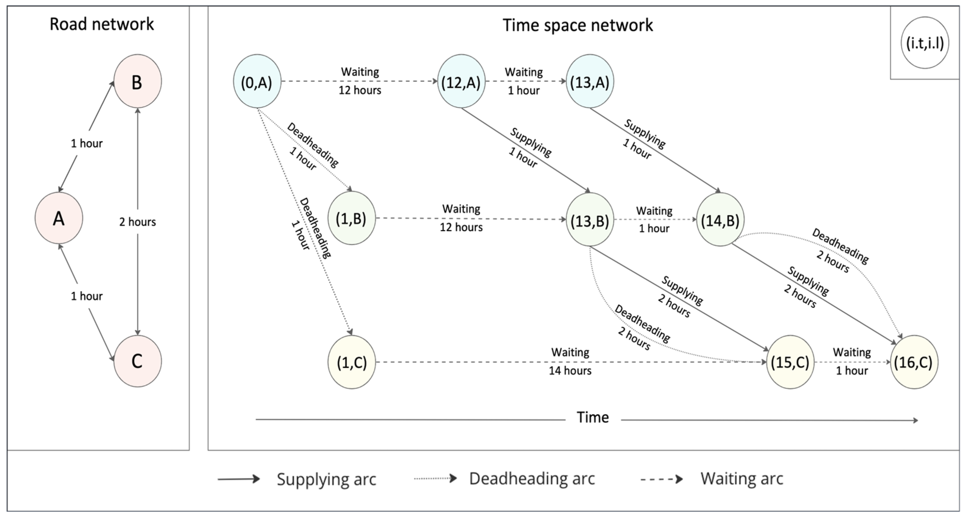
Figure 2.
Location of charging stations.

Figure 3.
(a) Average VKT. (b) Average travel time (minutes).

Figure 4.
Average profit and overhead cost.

Figure 5.
Average profit comparison.

Figure 6.
Average overhead-cost comparison.

Figure 7.
Average tour-time comparison.

Figure 8.
Average revenue comparison.

Figure 9.
Average travel-cost comparison.

Table 1.
Battery size and maximum range of EVs.
| Battery Capacity (kWh) | Max Range (km) | |
|---|---|---|
| Tesla Model S | 85 | 482 |
| Nissan Leaf | 24 | 161 |
| BMW i3 | 19 | 161 |
| Mitsubishi i-MiEV | 16 | 161 |
| Ford Focus | 23 | 161 |
| Honda Fit | 20 | 199 |
| Volkswagen e-Golf | 26.5 | 151 |
| BYD e6 | 57 | 302 |
| BYD Qin | 35 | 201 |
| DFM Venucia e30 | 24 | 175 |
Table 2.
Energy and charging time comparison.
| Energy Consumption Rate (Watt) | Supplied Energy (Watt) | Lost Energy (Watt) | Charging Time at CSs (Min) | |
|---|---|---|---|---|
| V2V Only | 1825.77 | 9363.047 | 463.84 | - |
| CSs Only | 2146.01 | 14,210.07 | - | 8.90 |
Table 3.
Deadheading, supplying, and waiting-time comparison.
| Deadheading Time (%) | Supplying Time (%) | Waiting Time (%) | |
|---|---|---|---|
| DP | 39.90 | 47.86 | 12.24 |
| CRP | 36.77 | 38.28 | 24.95 |
| HED | 50.40 | 42.13 | 7.48 |
Table 4.
Computation complexity comparison.
| Requester Count | DP | CBC | Greedy | |
|---|---|---|---|---|
| Runtime (ms) | Runtime (ms) | Runtime (ms) | Deviation from Optimal Solution (%) | |
| 10 | 115.66 | 210.32 | 0.095 | 11.23 |
| 20 | 338.90 | 427.66 | 0.645 | 9.19 |
| 30 | 532.89 | 597.80 | 0.132 | 25.74 |
| 40 | 994.92 | 1162.98 | 0.200 | 45.24 |
Disclaimer/Publisher’s Note: The statements, opinions and data contained in all publications are solely those of the individual author(s) and contributor(s) and not of MDPI and/or the editor(s). MDPI and/or the editor(s) disclaim responsibility for any injury to people or property resulting from any ideas, methods, instructions or products referred to in the content. |
© 2024 by the authors. Licensee MDPI, Basel, Switzerland. This article is an open access article distributed under the terms and conditions of the Creative Commons Attribution (CC BY) license (https://creativecommons.org/licenses/by/4.0/).
Share and Cite
MDPI and ACS Style
Alaskar, S.; Younis, M. Optimized Dynamic Vehicle-to-Vehicle Charging for Increased Profit. Energies 2024, 17, 2243. https://doi.org/10.3390/en17102243
AMA Style
Alaskar S, Younis M. Optimized Dynamic Vehicle-to-Vehicle Charging for Increased Profit. Energies. 2024; 17(10):2243. https://doi.org/10.3390/en17102243
Chicago/Turabian StyleAlaskar, Shorooq, and Mohamed Younis. 2024. "Optimized Dynamic Vehicle-to-Vehicle Charging for Increased Profit" Energies 17, no. 10: 2243. https://doi.org/10.3390/en17102243
Note that from the first issue of 2016, this journal uses article numbers instead of page numbers. See further details here.