DiTBN: Detail Injection-Based Two-Branch Network for Pansharpening of Remote Sensing Images

Abstract

Pansharpening is one of the main research topics in the field of remote sensing image processing. In pansharpening, the spectral information from a low spatial resolution multispectral (LRMS) image and the spatial information from a high spatial resolution panchromatic (PAN) image are integrated to obtain a high spatial resolution multispectral (HRMS) image. As a prerequisite for the application of LRMS and PAN images, pansharpening has received extensive attention from researchers, and many pansharpening methods based on convolutional neural networks (CNN) have been proposed. However, most CNN-based methods regard pansharpening as a super-resolution reconstruction problem, which may not make full use of the feature information in two types of source images. Inspired by the PanNet model, this paper proposes a detail injection-based two-branch network (DiTBN) for pansharpening. In order to obtain the most abundant spatial detail features, a two-branch network is designed to extract features from the high-frequency component of the PAN image and the multispectral image. Moreover, the feature information provided by source images is reused in the network to further improve information utilization. In order to avoid the training difficulty for a real dataset, a new loss function is introduced to enhance the spectral and spatial consistency between the fused HRMS image and the input images. Experiments on different datasets show that the proposed method achieves excellent performance in both qualitative and quantitative evaluations as compared with several advanced pansharpening methods.

1. Introduction

Some well-known remote sensing satellites, such as Ikonos, GeoEye-1, and WorldView-3, usually acquire two types of images: a low spatial resolution multispectral(LRMS) image with high spectral resolution and the panchromatic (PAN) image with high spatial resolution and low spectral resolution. These images have unilateral characteristics and cannot meet the needs of most practical applications. Thus, it is necessary to fuse the LRMS image and the PAN image to obtain a fused image that combines the complementary characteristics of two types of images. This fusion process is called pansharpening, which aims to obtain a fused image with rich spatial and spectral information by fusing an LRMS image and a PAN image in the same scene. Pansharpening is used in various fields related to remote sensing images, such as target detection, environmental monitoring, and object classification [1,2,3,4,5].

In recent years, pansharpening technology has made considerable progress. According to different basic models, the existing pansharpening techniques can be mainly divided into three categories: component substitution (CS) methods, multi-resolution analysis (MRA) methods, and model-based methods. The CS methods firstly separate the spatial information from the up-sampled LRMS image through a certain transformation, then replace the separated spatial information with the PAN image, and finally go through the inverse transformation to obtain a pansharpened image. This type of method is simple and fast, but the generated image usually has obvious spectral distortion. The representative CS methods include intensity–hue–saturation (IHS) transform [6], principal component analysis (PCA) [7], Gram–Schmidt transform (GS) [8], etc. The MRA methods are based on the assumption that the missing spatial information in the LRMS image can be inferred from the high-frequency information of the PAN image. It firstly obtains high-frequency components from PAN image through multi-resolution decomposition tools such as wavelet transform [9], high-pass filtering [10], Laplacian pyramid [11], etc., and then injects the component into the upsampled LRMS image. The fused image generated by such methods generally has higher spectral fidelity, but is prone to produce blurred details and artifacts.

Model-based methods have received more attention in recent years. A representative model is the convolutional neural network (CNN) in deep learning (DL). These methods construct the relationship between the source images and the ideal HRMS image and then make predictions through the trained model. The successful practices of CNN in many fields have inspired more and more researchers to use CNN for pansharpening. For example, Masi et al. [12] pioneered the use of CNN for pansharpening. In PNN, they firstly concatenated the upsampled LRMS and PAN images, and then utilized a simple three-layer network to fuse the concatenated data. To improve the network performance, Scarpa [13] introduced residual learning and L1 loss function based on PNN. Yang et al. [14] proposed a network called PanNet that performs a fusion process in the high-pass domain of the source images to enhance the structural consistency between the fused image and the source images. In addition, they introduced skip connections to deepen the network structure and maintain the spectral consistency between the fused image and the upsampled LRMS image. Liu et al. [15] proposed a two-stream fusion network (TFNet) that uses two sub-networks to extract features from LRMS and PAN images, respectively, and then fused the feature maps in the feature domain. Liu et al. [16] proposed a detail injection-based convolutional neural network (DiCNN) method for pansharpening the MS image, in which the details are formulated in end-to-end manner. DiCNN1 is one method of DiCNN, which extracts the details from the PAN image and the MS image. Deng et al. [17] proposed a new detail injection-based method named FusionNet, which learns the detail information from the difference between PAN images and upsampled LRMS images. Yang et al. [18] proposed a progressive cascaded deep residual network (PCDRN). PCDRN firstly performs a preliminary fusion on the upsampled LRMS image and the downsampled PAN image, and then further fuses the initial fused result with the original PAN image. The other CNN models have also made significant contributions in dealing with pan-sharpening problem and its related applications, including MSDRN [19], SSE-Net [20], MCANet [21], and MMDN [22]. Another famous deep learning model is Generative Adversarial Networks (GAN), which is widely applied in pansharpening. Liu et al. [23] proposed a remote sensing image pansharpening method based on GAN, which is named PSGAN. Ma et al. [24] proposed a unsupervised framework for pansharpening based a GAN, which aims to overcome the lack of ground truth and insufficient use of the panchromatic information. Benzenati et al. [25] proposed a network called as DI-GAN, which uses a GAN to acquire the optimal high frequency details to improve the fusion performance. Compared with the traditional pansharpening algorithms, the DL-based methods can effectively preserve the spectral information and spatial information in the source images and obtain a higher quality fused image.

Drawing on the detail injection strategy of the CS and MRA algorithms, a detail injection-based two-branch network (DiTBN (Code is available at https://github.com/Another1947/DiTBN) (accessed on 28 November 2022)) for pansharpening has been proposed. First, two parallel network branches are used to extract the features of two source images, and then the obtained feature information is continuously applied to the subsequent fusion process so as to make full use of the unique information contained in two source images. This strategy makes up for the loss of information in the fusion process and promotes the flow of information. Additionally, to alleviate the problems of high-frequency detail loss and spectral distortion of the fused images when using the common MSE loss function to train the network, this paper proposes a new loss function, which not only keeps the pixel value consistency with the reference image, but also imposes gradient constraints and spectral constraints on the fused image. The main contributions of this paper are summarized as follows:

(1) The proposed method constructs a detail injection-based two-branch network in the traditional CS or MRA fusion frameworks. The proposed network aims to adaptively acquire the optimal detail information, which can further enhance the spatial consistency between the fused image and the input PAN image. Compared to the end-to-end CNN-based pansharpening methods, the proposed method takes advantages of the traditional fusion framework and the CNN-based fusion framework, which produces robust and superior fusion performance.

(2) Many 1 × 1 convolution kernel is used to maintain spatial information of the input images or feature maps so as to reduce the parameters of the model and increase the diversity of features on different convolution kernels. This strategy can make the fusion network lighter and reduce the complexity of the network model.

(3) A new loss function is proposed. It not only includes the pixel value similarity between the fused image and the reference image, but also considers the spatial and spectral similarity between the fused image and two input images. The spectral loss and the spatial loss can make the fused images having better spectral and spatial quality.

The rest of this paper is organized as follows: Section 2 introduces the related work and background. Section 3 introduces the network structure and the loss function in detail. Experiments and performance evaluations are conducted in Section 4. Section 5 concludes this paper.

2. Background and Related Work

Let $\mathit{M}\in {\mathbb{R}}^{H/r\times W/r\times B}$ and $\mathit{P}\in {\mathbb{R}}^{H\times W}$ be the observed original LRMS and PAN images, respectively, where H and W respectively denote the height and width of the PAN image, r is the ratio of the spatial resolution between MS and PAN images, and B is the number of bands of the LRMS image. Let $\tilde{\mathit{M}}\in {\mathbb{R}}^{H\times W\times B}$ and $\widehat{\mathit{M}}\in {\mathbb{R}}^{H\times W\times B}$ be the interpolated LRMS image with the same size as the PAN image and the estimated pansharpened image, respectively. The task of pansharpening is to integrate the spectral information of the original MS image and the spatial information of the PAN image to obtain a fused image with the same spatial resolution as the PAN image and the same spectral resolution as the MS image.

2.1. The CS and MRA Methods

The CS methods are based on the assumption that the spatial information of the upsampled LRMS images can be separated by some transformation. After the spatial information is separated from the upsampled LRMS image, the spatial component is replaced with the PAN image, and then the pansharpened image is obtained through inverse transformation [26]. Mathematically, forward and inverse transforms can be simplified. The general CS model is expressed as follows:

$${\widehat{\mathit{M}}}_b={\tilde{\mathit{M}}}_b+g_b(\mathit{P}-\mathit{I}),b=1,2,\dots ,B$$

(1)

where ${\widehat{\mathit{M}}}_b$ and ${\tilde{\mathit{M}}}_b$ represent the bth band of $\widehat{\mathit{M}}$ and ${\tilde{\mathit{M}}}_b$, respectively; $g_b$ is the gain coefficient that regulates the amount of detail information injected into each band of the upsampled LRMS image; $\mathit{I}$ is the intensity component of the upsampled LRMS image, which is usually defined as a linear combination of all the upsampled LRMS image bands, i.e., $\mathit{I}={\sum }_{i-1}^B{w}_i\tilde{\mathit{M}}$ ($w_i$ is the weight coefficients). Most CS methods follow the above formula, so their key lies in the design of the weight coefficients $w_i$ and gain coefficients $g_b$, both of which significantly affect the performance of fused images. The CS methods usually suffer from severe spectral distortion due to changes in low spatial frequencies of the MS image or incomplete separation of spatial information during transformation.

The MRA methods assume that the missing spatial information in the upsampled LRMS image is available from the PAN image. These methods utilize multi-resolution analysis tools to separate high-frequency spatial information from the PAN image and inject it into the upsampled LRMS image. The process can be summarized in the following form:

$${\widehat{\mathit{M}}}_b={\tilde{\mathit{M}}}_b+g_b(\mathit{P}-{\mathit{P}}_{\mathit{L}}),b=1,2,\dots ,B$$

(2)

where ${\mathit{P}}_{\mathit{L}}$ is the low-pass filtered component of the PAN image. The key to the MRA methods is the acquisition of ${\mathit{P}}_{\mathit{L}}$ and the design of $g_b$. Due to the change of spatial information in the process of obtaining ${\mathit{P}}_{\mathit{L}}$, the MRA methods are prone to produce spatial distortion.

The acquisition of the intensity component in the CS methods, the acquisition of the low-frequency component of the PAN image in the MRA methods, and the gain coefficients all need to be manually designed, so these two methods have limited fusion performance.

2.2. The CNN Methods for Pansharpening

In recent years, deep learning technology is increasingly popular, and many researchers have applied deep learning technology to various fields and achieved considerable achievements. In image-related fields such as image classification [27], image super-resolution [28], image deblurring [29], object detection [30], etc., CNNs have been widely used. In recent years, CNNs have also been used for pansharpening. The idea of CNN-based pansharpening methods is to use the CNN model to construct the mapping relationship between the source images and the ideal HRMS image. The trained model can be acquired by minimizing the loss (such as L2 norm) between the pansharpened image and the corresponding ideal HRMS image. Finally, the trained model is used to predict the pansharpened image. If the L2 norm is used as the loss function, the above process can be described as

$$\begin{array}{cc}\hfill & \widehat{\mathit{\theta }}=\underset{\mathit{\theta }}{argmin}{∥\widehat{\mathit{M}}-\mathit{F}∥}_2^2=\underset{\mathit{\theta }}{argmin}{∥\phi (\tilde{\mathit{M}},\mathit{P},\mathit{\theta })-\mathit{F}∥}_2^2\hfill \\ \hfill & \widehat{\mathit{M}}=\phi (\tilde{\mathit{M}},\mathit{P},\widehat{\mathit{\theta }})\hfill \end{array}$$

(3)

where $\mathit{F}$ is the ideal HRMS image; $\phi (·)$, and $\mathit{\theta }$ represents the CNN model and its parameters.

Pansharpening can be regarded as a super-resolution reconstruction of the LRMS images. The difference is that pan-sharpening requires the PAN images as an auxiliary. Inspired by this, Masi et al. [12] pioneered the use of CNN for pansharpening (PNN). In their work, the upsampled LRMS and PAN images are concatenated and fed into a shallow network with a similar structure to Super-Resolution CNN (SRCNN) [28]. The network learns under the constraints of labels and then outputs the HRMS images through the trained model. In addition, the authors introduced the nonlinear radiometric indices to guide the learning process and improve network performance. Zhong et al. [31] proposed a strategy combining the SRCNN method and the GS method for pansharpening. They firstly used SRCNN to improve the spatial resolution of the LRMS image, and then used the GS method [8] to fuse the improved LRMS image and PAN image.

The nonlinear degree and fitting ability of the shallow network are limited. To address this problem, He et al. [32] proposed the idea of residual learning. They adopted a simple and effective structure called “skip connection” that identically maps the input of the residual unit to its output so that the residual unit only needs to learn the residual between the output and the input. Since the residual is generally sparse and the mapping within residual unit is more sensitive to changes in residuals than changes in output, the learning process becomes easier. In addition, the residual network can effectively alleviate the gradient disappearance problem caused by deepening the network, making it possible to build a deeper network. The proposal of residual learning promotes the development of CNN in related application fields. In the field of remote sensing, the CNNs that incorporate residual learning have achieved higher performance. For example, Wei et al. [33] proposed a deep residual network (DRPNN) in which residual learning was used, and the network structure was deepened. Yang et al. [14] proposed PanNet for fusion in the high-frequency domain. In PanNet, the high-pass filtered version of the source images are taken as inputs to preserve more details and edges. Then, a deep network composed of multiple residual units is employed to perform feature extraction and feature fusion on the input images. Finally, the upsampled LRMS image is added to the network output through skip connection to obtain the final fused image that can effectively preserve spectral information. Shao et al. [34] proposed a two-branch network that employed a deeper network to fully extract spatial features from PAN images, and a shallower network to extract features from upsampled LRMS images. Then, the feature maps of two images are concatenated and fused through a convolutional layer to obtain a detail image. Finally, the upsampled LRMS image is added to the residual image through skip connection to obtain the fused image. Yang et al. [18] proposed a progressive cascaded deep residual network (PCDRN). In PCDRN, the upsampled LRMS image by a ratio of 2 and the downsampled PAN image by a ratio of 2 are fed into a residual network to obtain a preliminary fusion result. Then, the fusion result is upsampled by a ratio of 2 and fused with the PAN image to obtain the final fused HRMS image. Compared with traditional CS and MRA methods, these CNN-based pansharpening methods achieve a better balance between spectral quality and spatial quality and obtain higher performance.

3. Detail Injection-Based Two-Branch Network

3.1. Motivation

According to the introduction in Section 2.1, the CS and MRA methods have one thing in common, i.e., the details are firstly obtained from the PAN image, and then they are injected into the upsampled LRMS image to obtain the HRMS image, which can be mathematically described as

$$\begin{array}{cc}\hfill {\widehat{\mathit{M}}}_b& \hfill ={\tilde{\mathit{M}}}_b+g_b\mathit{d}\hfill \\ \hfill & \hfill ={\tilde{\mathit{M}}}_b+{\mathit{D}}_b\hfill \end{array}$$

(4)

where $\mathit{d}$ represents the details obtained from the PAN image, and ${\mathit{D}}_b$ represents the details that need to be injected into the upsampled LRMS image. Equations (1) and (2) indicate that the details from the PAN image are obtained by linear models (linear combination or filtering). However, this assumption has not been confirmed. Meanwhile, there is overlap between the spectral responses of each band in the MS image. It may not be reasonable for injecting details according to Equation (4). On the one hand, the CNN can effectively capture the features of the input images and build a model with a high degree of nonlinearity. On the other hand, this approach eliminates the need for the design of injection gains, and it automatically adjusts the injected details to adapt to the expected output by learning.

Most of the existing CNN-based pansharpening methods regard pansharpening as an image super-resolution problem, i.e., the upsampled LRMS and PAN images are taken as inputs to directly learn the mapping between the input and the desired HRMS image. However, these methods ignore the difference between two source images. As an image fusion problem, pansharpening should make full use of the spatial information in the PAN image and inject the required parts into the upsampled LRMS image. To better mine and utilize the information in the source images, this paper considers extracting features from MS and PAN images separately, and then fuses the features of both to reconstruct a pansharpened image. In addition, to preserve edges and details and enhance the structural consistency between the PAN image and the HRMS images, this paper uses the high-frequency content of PAN images as one of the inputs [14].

3.2. The Network Architecture

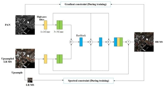
The framework of the proposed method for pansharpening is shown in Figure 1. The implementation of the proposed framework includes three stages: feature extraction, feature fusion, and HRMS image reconstruction. First, the LRMS image is upsampled to the same size as the PAN image, and the high-frequency content of the PAN image, denoted as ${\mathit{P}}_H$, is obtained by subtracting its low-pass version from the PAN image. The upsampled LRMS image and the high-frequency content of the PAN image are used as inputs.

In the feature extraction stage, two sub-networks composed of three consecutive convolutional layers are employed to extract the features from the high-frequency component of the PAN image and the upsampled LRMS image, respectively. Specifically, the first layer adopts a 1 × 1 kernel to preserve the spatial information of the inputs and reduce the number of model parameters. Let ${\mathit{F}}_P$ and ${\mathit{F}}_M$ be the feature maps of two images as ${\mathit{F}}_P$ and ${\mathit{F}}_M$, respectively. The output feature maps of the l-th layer can be expressed as

$$\begin{array}{cc}\hfill & {\mathit{F}}_P^{\left(l\right)}={\mathit{f}}_P^{\left(l\right)}\left({\mathit{P}}_H\right)\hfill \\ \hfill & {\mathit{F}}_M^{\left(l\right)}={\mathit{f}}_M^{\left(l\right)}\left(\tilde{\mathit{M}}\right),l=1,2,3\hfill \end{array}$$

(5)

where ${\mathit{f}}_P^{\left(l\right)}$ and ${\mathit{f}}_M^{\left(l\right)}$ represent the networks composed of the first layers of the feature extraction sub-networks of ${\mathit{P}}_H$ and $\tilde{\mathit{M}}$, respectively.

Next, the extracted feature maps ${\mathit{F}}_P^{\left(3\right)}$ and ${\mathit{F}}_M^{\left(3\right)}$ are concatenated along the channel direction and fed into the feature fusion sub-network. The feature fusion network integrates the feature information from the high-frequency component of the PAN image and the upsampled LRMS image to obtain the fused feature maps. It performs further feature extraction on the fused feature maps. Considering that the spatial information of the reconstructed HRMS image mainly comes from the PAN image and the spectral information mainly comes from the upsampled LRMS image, it is difficult to recover the texture details since the high-level features encode the semantic and abstract information of the image. Thus, this paper considers to continuously utilize the feature maps from the high-frequency component of the PAN image and upsampled LRMS image in the process of feature fusion through skip connections. This iterative strategy can compensate for the loss of spectral and spatial information in the feature fusion process and continuously inject spectral and spatial information into the fused feature maps, which is conducive to the reconstruction of HRMS images. The feature fusion sub-network consists of three consecutive residual units, each of which consists of a 1 × 1 convolutional layer, two 3 × 3 convolutional layers, and a skip connection. Its structure is shown in the dashed box as shown in Figure 1. The first residual unit receives the output feature maps of two feature extraction sub-networks as input. In addition to receiving the output of the previous residual unit as input, the second and third residual units also receive the feature maps from the output of the first convolutional layer of two feature extraction sub-networks. The output ${\mathit{F}}_i$ of the i-th residual unit can be expressed as

$${\mathit{F}}_i=\left\{\begin{array}{cc}{R}_i([{\mathit{F}}_P^{\left(3\right)},{\mathit{F}}_M^{(3)}])& i=1\\ R_i([{\mathit{F}}_{i-1},{\mathit{F}}_P^{(1)},{\mathit{F}}_M^{(1)}])& i=2,3\end{array}\right.$$

(6)

where $[·]$ represents the concatenate operation along the channel dimension, and $R_i$ represents the mapping function of the residual unit.

The feature fusion sub-network outputs a high-level fused feature map ${\mathit{F}}_3$, which is fed into the image reconstruction sub-network to obtain a detail image. First, a convolutional layer with 1 × 1 kernel is used to reduce the channel dimension of ${\mathit{F}}_3$. Then, a convolutional layer with 3 × 3 kernel is used to map the dimensionality-reduced feature map to the detail image that needs to be compensated to the upsampled LRMS image. The detail image can be represented as

$$\mathit{D}=H\left({\mathit{F}}_3\right)$$

(7)

where H represents the image reconstruction sub-network composed of the above two convolutional layers. Finally, the upsampled LRMS image $\tilde{\mathit{M}}$ is passed to the output of the image reconstruction sub-network through skip connection. Thus, the obtained HRMS image is

$$\widehat{\mathit{M}}=\tilde{\mathit{M}}+\mathit{D}$$

(8)

3.3. The Loss Function

In fact, the ideal HRMS image does not exist. For this reason, Wald et al. [35] provided a feasible training scheme, i.e., the reduced-resolution PAN image and LRMS image are used as network inputs, and the original LRMS image is used as the reference. Denote the PAN and LRMS images at reduced resolution as $\mathit{p}$ and $\mathit{m}$, respectively, and denote the corresponding network output as $\tilde{\mathit{m}}$. A dataset with N pairs of training samples can be represented as ${\left\{{\mathit{P}}^{\left(i\right)},{\mathit{m}}^{\left(i\right)},{\mathit{M}}^{\left(i\right)}\right\}}_{i=1}^N$.

Many CNN-based pansharpening methods aim to minimize the difference between the network output $\widehat{\mathit{m}}$ and the corresponding reference image $\mathit{M}$, i.e.,

$$minL(\widehat{\mathit{m}}-\mathit{M})$$

(9)

where L represents the loss function. With a reference image, pansharpening can be regarded as a regression problem. The commonly used loss function in regression problems is mean square error (MSE). The loss function can be expressed as

$$L_M=\frac{1}{N}\sum _{i=1}^N{∥{\widehat{\mathit{m}}}^{\left(i\right)}-{\mathit{M}}^{\left(i\right)}∥}_2^2$$

(10)

Although the MSE loss function has achieved good performance in most CNN-based pansharpening methods, some problems still exist. There is usually a loss of high-frequency details in the fused image, such as the artifact phenomenon [36], especially for some small objects in the image. Meanwhile, there is a spectral performance gap between the fused image and the reference image, which is more obvious for small objects. Furthermore, the MSE loss function only considers the pixel value loss between the output pansharpened image by the network and the reference image. It ignores the spatial or spectral loss and does not consider the consistency between the pansharpened image and the source images. Therefore, the loss function can be further improved. Focusing on these problems, this paper proposes a new loss function. In addition to the MSE loss between the sharpened HRMS image and the reference image, the proposed loss function also includes two other loss terms: the spatial constraint of the PAN image for the pansharpened image, and the spectral constraint of the LRMS image for the pansharpened image.

The variational methods applied to pansharpening usually model the energy function of spatial correlation between PAN and HRMS images and the energy function of the spectral correlation between LRMS and HRMS images. They optimize these functions to obtain the sharpened HRMS image. Based on the idea of the variational methods, this paper adds spatial and spectral constraints on the sharpened HRMS images during network training. Some variational methods [37] believe that the gradient of each spectral band of the sharpened HRMS image should be consistent with that of the PAN image, i.e.,

$$▽{\widehat{\mathit{M}}}_b=▽\mathit{P},b=1,2,\dots ,B$$

(11)

where ▽ is the gradient operator, and it is defined as $▽\mathit{x}=\sqrt{{\mathit{x}}_x^2+{\mathit{x}}_y^2}$ for a single-band image, where ${\mathit{x}}_x$ and ${\mathit{x}}_y$ represent the horizontal and vertical gradients, respectively. Accordingly, this paper imposes spatial information constraints on the sharpened HRMS image during the network training phase, which are defined as

$$L_S=\frac{1}{N}\sum _{i=1}^N{∥▽{\widehat{\mathit{m}}}^{\left(i\right)}-repmat(▽{\mathit{p}}^{\left(i\right)})∥}_2^2$$

(12)

where $repmat$ is the operation of extending the gradient image of $\mathit{p}$ along the band direction to the same number of bands as $\widehat{\mathit{m}}$. Equation (12) forces the gradient of the sharpened HRMS image to be consistent with that of the PAN image, thereby enhancing the spatial consistency between the HRMS and the PAN image.

Typically, Wald’s protocol refers to the synthesis property [35,38]. Meanwhile, Wald also proposed a consistency property, i.e., a spatially degraded pansharpened image should be as consistent as possible with the observed LRMS image. For better results, the implementation of spatial degradation should use a filter that matches the modulation transfer function (MTF) of the sensor from which the LRMS image is acquired. To improve the consistency between the sharpened HRMS image and the LRMS image, the input LRMS image is utilized to impose a spectral constraint on the output HRMS image in the training process according to the consistency property, which is defined as

$$L_{\lambda }=\frac{1}{N}\sum _{i=1}^N{∥{\mathit{f}}_{degrade}({\widehat{\mathit{m}}}^{\left(i\right)}-{\mathit{m}}^{\left(i\right)})∥}_2^2$$

(13)

where ${\mathit{f}}_{degrade}$ represents the use of a spatial degradation operation with MTF filtering [38] on the image. By the constraint of Equation (13), the output image after spatial degradation will be forced to be consistent with the input LRMS image, and the spectral consistency of two images will be enhanced.

In summary, in addition to the MSE loss between the sharpened HRMS image and the reference image, the above spatial constraint and spectral constraint are imposed as auxiliary. In addition, to avoid overfitting, L2 regularization is applied for weight decay. Denote the weight decay coefficient as $\gamma$. Combining Equations (10)–(12), the total loss function is

$$L=L_M+\alpha ·L_S+\beta ·L_{\lambda }+\gamma {∥\mathit{\theta }∥}_2^2$$

(14)

where $\alpha$ and $\beta$ are the weight coefficients of the spatial loss term $L_S$ and the spectral loss term $L_{\lambda }$, and $\mathit{\theta }$ is the model parameters. Different types of loss terms are normalized by the number of elements in a single training sample (i.e., height × width × channels).

4. Experiments

4.1. Experimental Datasets

To evaluate the performance of DiTBN, this paper selects datasets from three satellites, i.e., Ikonos, GeoEye-1, and WorldView-3, to test the model. The Ikonos satellite is the first civil satellite with a resolution better than 1 m in the world. It provides the PAN images with a spatial resolution of 1 m and the LRMS images with a spatial resolution of 4 m. The LRMS images include spectral information in four bands of red, green, blue, and near-infrared, and the PAN images only have a single band. The GeoEye-1 satellite carries two sensors, in which the panchromatic sensor acquires the PAN images with a spatial resolution of 0.5 m, and the multispectral sensor acquires the LRMS images with a spatial resolution of 2 m. The LRMS images also have spectral information in four bands of red, green, blue, and near-infrared. The WorldView-3 satellite provides the PAN images with a spatial resolution of 0.31 m and the LRMS images with a spatial resolution of 1.24 m. In addition to the four standard spectral bands, the LRMS images also include four bands of coastal, yellow, red edge, and near-infrared. The radiometric resolution of three types of satellite images is 11 bits. The main characteristics of three satellites are listed in

Table 1. The main characteristics of three satellites.

Satellites	Spectral Range/nm									Spatial Resolution/m
	Coastal	Blue	Green	Yellow	Red	Red Edge	Nir	Nir2	PAN	PAN	MS
Ikonos	-	450–530	520–610	-	640–720	-	760–860	-	450–900	1	4
GeoEye-1	-	450–510	510–580	-	655–690	-	780–920	-	450–900	0.5	2
WorldView-3	400–450	450–510	510–580	585–625	630–690	705–745	770–895	860–1040	450–800	0.31	1.24

.

For each type of satellite source data, this paper first segments it into 200 × 200 LRMS image patches and corresponding 800 × 800 PAN image patches. The image patches do not overlap each other. Then, these image patches are randomly divided into training data, validation data, and test data at a ratio of 8:1:1. During the training phase, this paper follows the Wald’s protocol to generate datasets, i.e., using the spatially degraded source images as inputs and using the original LRMS image as the reference image. The subsampling factor for different datasets is four. For training data and validation data, spatial degradation with MTF filtering is performed on each group of source image patches, and then the degraded images (inputs) and the source LRMS images (reference image) are cropped to small-size image patches in a certain stride to obtain a large number of training and validation datasets. The division of each type of dataset is shown in

Table 2. The division of the dataset (The sizes of the LRMS and PAN images).

Satellites	Number of Source Images/Group	Data Type	Number of Groups	Patch Number
Ikonos	240 × (200 × 200, 800 × 800)	Train	192	12,288 × (8 × 8, 32 × 32)
		Valid	24	1536 × (8 × 8, 32 × 32)
		Test	24	24 × (50 × 50, 200 × 200)
GeoEye-1	250 × (200 × 200, 800 × 800)	Train	200	12,800 × (8 × 8, 32 × 32)
		Valid	25	1600 × (8 × 8, 32 × 32)
		Test	25	25 × (50 × 50, 200 × 200)
WorldView-3	250 × (200 × 200, 800 × 800)	Train	200	12,800 × (8 × 8, 32 × 32)
		Valid	25	1600 × (8 × 8, 32 × 32)
		Test set	25	25 × (50 × 50, 200 × 200)

. This paper interpolates the LRMS image using a polynomial interpolation method [39] with 23 coefficients.

4.2. Implement Details

In this article, the Tensorflow framework is used to build, train, and test the network model in the environment of Python 3.6. The training is performed on a computer equipped with an NVIDIA Quadro P4000. The loss function is optimized by the Adam [40] method. The maximum number of iterations is set to 100,100. The initial learning rate is set to 0.001 and decays by $50\%$ every 20,000 iterations. The training batch size is set to 16, and the weight decay coefficient is set to ${10}^{-5}$. The weight coefficients of the spatial loss term $L_s$ and the spectral loss term $L_{\lambda }$ are set to 0.1 and 1, respectively.

4.3. The Evaluation Indicators and Comparison Algorithms

In addition to the visual evaluation of the fused images, some quantitative evaluation indicators are also used. Performance evaluation is performed on two scales: reduced-resolution scale (also known as simulated experiments) and full-resolution scale (also known as real experiments). For the former, this paper selects six widely used indicators, including spectral angle mapper (SAM) [41], erreur relative globale adimensionnelle de synthèse (ERGAS) [42], relative average spectral error (RASE) [43], spatial correlation coefficient (SCC) [44], universal image quality index (Q) [45], and structural similarity (SSIM) index [46]. For the latter, four indicators are used, including spectral distortion index $D_{\lambda }$, spatial distortion index $D_S$, quality no reference index (QNR) [47], and SAM.

In this paper, eight popular algorithms are taken for comparison. The comparison algorithms of the CS methods include the Gram–Schmidt mode 2 algorithm with a generalized Laplacian pyramid (GS2-GLP) [11], the robust band dependent spatial detail (BDSD-PC) [48]. The comparison algorithms of the MRA methods include the generalized Laplacian pyramid with an MTF-matched filter (MTF-GLP) [11], the additive wavelet luminance proportional with haze correction (AWLP-H) [49]. The comparison algorithms of the CNN-based methods include a deep network for pansharpening (PanNet) [14], first detail injection CNN (DiCNN1) [16], FusionNet [17], and TFNet [15]. The TFNet method is tested on the Ikonos and GeoEye-1 datasets. As for the implementation of the first four traditional algorithms, the toolbox provided by Vivone et al. [50] is used. The implementation codes of the PanNet, FusionNet and TFNet methods can be found on open-source websites (Code link: https://xueyangfu.github.io/; https://github.com/liangjiandeng/FusionNet; https://github.com/liouxy/tfnet_pytorch (accessed on 1 May 2022)). As to the DiCNN1 method, the reproduced version provided by Deng et al. [17] is used. To be fair, all CNN-based methods operate under the same hardware and software environmental conditions. Meanwhile, since most CNN-based methods do not provide trained models, this paper retrains the CNN-based comparison algorithms using the same dataset as applied to the proposed network.

4.4. The Ablation Study of Different Network Structures

The High-Pass Filtering (HPF) is used on the input PAN image, and the feature map reuse is implemented in our network structure. To explore the impact of different network settings on model performance, this paper performs an ablation study on the simulated Ikonos dataset. As shown in Figure 1, HPF2 means that the HPF is applied on two input images at the same time. HPF1 means that the HPF is only applied on the input PAN image. Reuse2 denotes that the feature maps from two branches are reused. Reuse1 denotes that the feature maps of the PAN branch are reused. “No reuse” means that the feature maps are not reused. The model performance of the above settings is compared under four different combinations, where “HPF1, reuse2” indicates the settings used in the proposed method.

Table 3. Ablation study of different network structures on the Ikonos dataset.

	SAM↓	ERGAS↓	RASE↓	SCC↑	Q↑	SSIM↑
HPF2, reuse2	2.6461	1.8537	7.5817	0.9472	0.8691	0.9543
HPF1, reuse2	2.5097	1.7846	7.2815	0.9530	0.8737	0.9578
HPF1, no reuse	2.5196	1.7861	7.2836	0.9531	0.8739	0.9577
HPF1, reuse1	2.5298	1.7929	7.3119	0.9530	0.8747	0.9577

lists the average values of all the indicators, the best value is marked in bold.

It can be seen from Table 3 that the combined setting adopted by the proposed method achieves the best results in spectral performance and competitive results in spatial performance. In the case of reusing the feature maps of both branches, only using the HPF on the input PAN image shows better performance than using the HPF on both input images. This is perhaps because using the HPF on the input MS image will filter out the low-frequency information. However, using only a small amount of high-frequency information that is not essential to the reconstructed detail image may lead to redundant information, which in turn causes the distortion of the fused image. Reusing feature maps from both branches obtains the best spectral performance with only HPF on the input PAN image. This indicates that only reusing the feature maps of the input PAN image may inject too much spatial information, which results in spectral distortion of the fused image. Furthermore, simultaneously reusing the feature maps of the input MS image can effectively transfer the low-frequency information contained in it to the feature fusion process, which can improve the spectral quality of the fused image. Therefore, in the case of using the HPF on the input PAN image, reusing the feature maps of the MS image branch can improve the performance when only the feature maps of the PAN image branch are reused, which illustrates the effectiveness of reusing the feature maps of two branches simultaneously.

4.5. The Ablation Studies of the Proposed Loss Function and Kernel Size

This paper introduces a loss function that constrains the spectral and spatial information of the fused image according to the information of the input images. In addition to the commonly used MSE loss, it also includes the spatial constraint of the PAN image to the sharpened HRMS image and the spectral constraint of the LRMS image to the sharpened HRMS image. To verify the effectiveness of the proposed loss function, ablation studies are conducted on the simulated Ikonos dataset. Under the same model structure, the MSE loss function, the loss function without $L_s$, the loss function without $L_{\lambda }$, and the proposed loss function are used, respectively, to conduct experiments. The test results are listed in

Table 4. Ablation study of different loss functions on the Ikonos dataset.

Loss	SAM↓	ERGAS↓	RASE↓	SCC↑	Q↑	SSIM↑
The MSE loss function	2.5445	1.8060	7.3646	0.9518	0.8718	0.9569
The loss function without $L_s$	2.5191	1.7962	7.3250	0.9526	0.8733	0.9575
The loss function without $L_{\lambda }$	2.5263	1.7993	7.3456	0.9525	0.8738	0.9571
The proposed loss function	2.5097	1.7846	7.2815	0.9530	0.8737	0.9578

, the best value is marked in bold.

It can be seen from Table 4 that training the network with the proposed loss function improves the model performance in both spatial and spectral quality as compared to training the network with the MSE loss function. This is because the MSE loss between the fused image and the reference image only considers the similarity of pixel values. Although it can constrain the spatial and spectral information of the fused image to a certain extent, it does not explicitly point out the spatial and spectral consistency between the fused image and the input images. In addition, the loss function without $L_s$ and the loss function without $L_{\lambda }$ are compared in this experiment. The quantitative assessment results demonstrate that the introduction of spatial and spectral constraints in the proposed loss function makes the model obtain more spatial and spectral clues from the input PAN and LRMS images in the optimization process and strengthens the spatial and spectral consistency between the fused image and the input images.

In this subsection, we also give the ablation study of different kernel sizes, i.e., 1 × 1 and 3 × 3.

Table 5. Ablation study of different kernel sizes on the Ikonos dataset.

Kernel Size	SAM↓	ERGAS↓	RASE↓	SCC↑	Q↑	SSIM↑
1 × 1	2.5097	1.7846	7.2815	0.9530	0.8737	0.9578
3 × 3	2.5103	1.7870	7.2904	0.9531	0.8743	0.9577

lists the quantitative assessment results on the Ikonos dataset, the best value is marked in bold. It can be observed that the proposed method with 1 × 1 kernel size has better fusion performance. In addition, the kernel size 1 × 1 can make the fusion network have less parameters.

4.6. Performance Evaluation at Reduced-Resolution Scale

In this subsection, the proposed method and the comparison algorithms are evaluated at the reduced-resolution scale. The experiments at the reduced scale generate datasets based on Wald’s protocol. Figure 2 shows the fusion results of different algorithms on a group of Ikonos reduced-resolution test images. To better illustrate the difference between the fused images and the reference image, the residual images are shown in Figure 3. It can be observed from Figure 2 and Figure 3 that the residual image of the GS2-GLP method exhibits serious spectral distortion, especially for the red buildings. In addition, it shows some edge and texture information, indicating that the fused image has spatial distortion. The residual image of the BDSD-PC algorithm also shows serious spectral distortion and spatial distortion. The fused images of the AWLP-H and MTF-GLP algorithms show a certain blurring that is reflected in the corresponding residual images. In addition, they are accompanied by some spectral distortion. Compared with the residual images of traditional algorithms, those obtained by CNN-based methods exhibit less residual information, indicating that CNN-based methods produce fused images with higher spectral and spatial quality. Specifically, the PanNet, DiCNN1, and TFNet methods produce slight spectral distortion and spatial distortion, while the FusionNet method and our proposed method produce the least distortion.

To give an objective evaluation of all algorithms,

Table 6. Comparison of indicator evaluation results on the reduced-resolution Ikonos dataset.

	Methods	SAM↓	ERGAS↓	RASE↓	SCC↑	Q↑	SSIM↑
The indicator values in Figure 2	GS2-GLP	3.3848	3.3752	13.0279	0.9331	0.9350	0.9191
	BDSD-PC	3.5979	3.5113	13.5917	0.9300	0.9308	0.9171
	AWLP-H	3.1770	3.4612	13.3689	0.9326	0.9337	0.9248
	MTF-GLP	3.5667	3.8054	14.6481	0.9301	0.9207	0.9057
	PanNet	2.6250	2.2085	8.5422	0.9783	0.9618	0.9581
	DiCNN1	2.5199	2.1116	8.1636	0.9811	0.9621	0.9612
	FusionNet	2.4568	2.0755	8.0386	0.9815	0.9633	0.9628
	TFNet	2.7608	2.6473	10.2455	0.9699	0.9509	0.9468
	Proposed	2.3822	2.0604	7.9741	0.9817	0.9644	0.9636
The average indicator values	GS2-GLP	3.8824	2.6749	10.7669	0.8818	0.7867	0.9070
	BDSD-PC	3.8636	2.6820	10.7902	0.8885	0.7965	0.9117
	AWLP-H	3.5207	2.6405	10.6203	0.8931	0.8098	0.9201
	MTF-GLP	4.0959	2.7863	11.7074	0.8716	0.7747	0.8959
	PanNet	2.6712	1.8804	7.6997	0.9444	0.8673	0.9527
	DiCNN1	2.6529	1.8696	7.6126	0.9466	0.8671	0.9535
	FusionNet	2.5791	1.8169	7.4268	0.9500	0.8687	0.9562
	TFNet	3.0225	2.2030	8.9109	0.9298	0.8392	0.9401
	Proposed	2.5097	1.7846	7.2815	0.9530	0.8737	0.9578

lists the indicator values of the fusion results in Figure 2 and the average indicator values of 24 groups of test images on the Ikonos dataset, where the best value is marked in bold and the second best value is underlined. As shown in Table 6, for the image shown in Figure 2, our analysis of the fused images is basically consistent with the indicator values. For all test images, the CNN-based methods have better performance than the traditional algorithms. Among the traditional algorithms, AWLP-H achieves the leading performance. The proposed algorithm obtains the best results, indicating that it can effectively reduce the spectral and spatial distortions in the fusion process.

Figure 4 and Figure 5 respectively show the fusion results and the corresponding residual images of a group of reduced-resolution samples on the GeoEye-1 dataset. It can be seen from the figures that the fused image of the BDSD-PC method produces serious spectral distortion, especially in the water area and vegetation area, and the vegetation area is over-saturated. The GS2-GLP also produces some spectral distortions, especially in the vegetation area below the image. The fused images of the AWLP-H and MTF-GLP methods have better spectral quality. However, there is some blurring, especially for the MTF-GLP method. Compared with the fused images of the traditional algorithms, those of the CNN-based methods are closer to the ground truth image in spectrum and spatial. However, some spectral and spatial distortions can be still observed from the residual images.The PanNet, DiCNN1 and TFNet methods show relatively more residual information, while FusionNet and the proposed method reflect less residual information.

To give an objective evaluation of the fusion results in Figure 4 and the performance of each algorithm on the GeoEye-1 dataset,

Table 7. Comparison of indicator evaluation results on the reduced-resolution GeoEye-1 dataset.

	Methods	SAM↓	ERGAS↓	RASE↓	SCC↑	Q↑	SSIM↑
The indicator values in Figure 4	GS2-GLP	3.8439	4.1591	20.3177	0.7741	0.8599	0.9256
	BDSD-PC	5.3266	3.6951	17.9216	0.8355	0.8640	0.9230
	AWLP-H	3.6043	3.8770	18.0543	0.8226	0.8759	0.9313
	MTF-GLP	3.8435	4.1684	20.2097	0.7749	0.8594	0.9251
	PanNet	2.0523	1.9989	9.1007	0.9469	0.9063	0.9727
	DiCNN1	1.8240	1.9016	8.7054	0.9535	0.9190	0.9761
	FusionNet	1.8441	1.8955	8.5859	0.9535	0.9110	0.9767
	TFNet	2.1218	2.2806	10.3625	0.9315	0.8752	0.9675
	Proposed	1.6372	1.7813	8.1048	0.9581	0.9216	0.9793
The average indicator values	GS2-GLP	3.2744	2.8539	13.3318	0.8168	0.8206	0.8929
	BDSD-PC	3.0881	2.5465	11.8565	0.8794	0.8601	0.9222
	AWLP-H	2.4347	2.3470	10.8151	0.9124	0.8789	0.9427
	MTF-GLP	2.9326	2.7003	12.2147	0.8766	0.8431	0.9186
	PanNet	1.5137	1.4808	6.7133	0.9609	0.9320	0.9691
	DiCNN1	1.4790	1.4567	6.7126	0.9617	0.9326	0.9704
	FusionNet	1.4653	1.4657	6.5833	0.9631	0.9294	0.9708
	TFNet	1.6539	1.6889	7.6106	0.9499	0.9137	0.9633
	Proposed	1.3642	1.3772	6.2741	0.9663	0.9380	0.9734

lists the indicator values of the fusion results in Figure 4 and the average indicator values of the 25 groups of test images on the GeoEye-1 dataset, where the best value is marked in bold and the second best value is underlined. All subsequent table expressions follow this instruction. According to Table 7, among the traditional algorithms, the AWLP-H algorithm obtains competitive results on the image shown in Figure 4, and it obtains leading results in terms of average indicator values. The CNN-based methods generally achieve better results than the traditional algorithms. Specifically, DiCNN1 and FusionNet compete fiercely, while our method achieves the best results.

Figure 6 and Figure 7 show an example of the fusion results on the reduced-resolution WorldView-3 dataset and the corresponding residual images, respectively. It can be seen that the BDSD-PC algorithm produces severe spectral distortion, especially on land areas and red buildings. The GS2-GLP algorithm also produces some spectral distortion, mostly for red and blue buildings. The fused image of the AWLP-H algorithm has more natural color but lacks more texture information. The MTF-GLP algorithm suffers from spectral distortion on red and blue buildings, as well as some detail blurring. The CNN-based methods all suffer from slight spectral distortion on red buildings. The proposed method produces the least spectral and spatial loss.

Table 8. Comparison of indicator evaluation results on the reduced-resolution WorldView-3 dataset.

	Methods	SAM↓	ERGAS↓	RASE↓	SCC↑	Q↑	SSIM↑
The indicator values in Figure 6	GS2-GLP	5.2773	3.6583	10.9792	0.9000	0.9411	0.9060
	BDSD-PC	5.5379	3.9007	11.9896	0.8981	0.9402	0.9034
	AWLP-H	5.4564	3.9955	11.3766	0.8769	0.9401	0.9099
	MTF-GLP	5.1129	3.6498	11.0362	0.8957	0.9421	0.9090
	PanNet	3.4405	2.2765	6.8848	0.9594	0.9785	0.9598
	DiCNN1	3.2887	2.1864	6.6807	0.9643	0.9803	0.9634
	FusionNet	3.2403	2.1687	6.6682	0.9652	0.9803	0.9642
	Proposed	3.0829	2.0869	6.2865	0.9665	0.9824	0.9668
The average indicator values	GS2-GLP	5.2773	4.4745	10.0756	0.8602	0.8972	0.9125
	BDSD-PC	6.3906	4.6631	10.5381	0.8659	0.8937	0.9064
	AWLP-H	4.9514	4.5022	10.2020	0.8651	0.9094	0.9263
	MTF-GLP	5.1142	4.4390	9.9565	0.8587	0.8998	0.9184
	PanNet	3.3803	2.5651	6.1025	0.9590	0.9503	0.9681
	DiCNN1	3.2656	2.4916	5.9104	0.9628	0.9520	0.9700
	FusionNet	3.1362	2.4790	5.9783	0.9642	0.9518	0.9709
	Proposed	2.9323	2.3374	5.6141	0.9674	0.9556	0.9737

lists the indicator values of the fusion results in Figure 6 and the average indicator values of 25 groups of test images on the WorldView-3 dataset. As to the images shown in Figure 6, it can be observed that the performance of four traditional algorithms is very close. The proposed method and the FusionNet method achieve the best and sub-best results, respectively. For all the test images, the performance of four traditional algorithms is still relatively close. Four CNN-based methods generally perform better than the traditional algorithms. In particular, the proposed method obtains the best results in terms of SAM, ERGAS, RASE, SCC, Q, and SSIM.

4.7. Performance Evaluation at Full-Resolution Scale

For practical applications, it is necessary to conduct experiments on remote sensing images at full-resolution scale. In this subsection, the original datasets are used as the test data to be fused. The performance of each algorithm is evaluated through visual evaluation and objective assessment metrics. Since there is no reference image, the values of SAM indicator in the quantitative evaluation are calculated between the spatially degraded fused images and the original LRMS images.

Figure 8 shows the fusion results of each algorithm on a group of samples on the full-resolution Ikonos dataset. The area enclosed by a green box is enlarged and placed at the right bottom of each image. Compared with the upsampled LRMS image, the fused images produced by all methods show a high spatial quality improvement, which can be easily observed from the local enlarged areas at the bottom of the images. The GS2-GLP algorithm produces some spectral distortion, mainly in vegetated areas. The fused image of the BDSD-PC algorithm exhibits over-saturation, especially for red tones. The MTF-GLP algorithm also produces some spectral distortion. Compared with the previous algorithms, the fused image of AWLP-H has more natural colors. The FusionNet method exhibits some artifacts at the edges of buildings in the local enlarged area. Several other CNN-based methods obtain relatively similar spectral and spatial features, which are close to those of the upsampled LRMS image and PAN image.

Table 9. Comparison of indicator evaluation results on the full-resolution Ikonos dataset.

	Methods	SAM↓	QNR↑	${\mathit{D}}_{\mathit{\lambda }}$↓	${\mathit{D}}_{\mathit{S}}$↓
The indicator values in Figure 8	GS2-GLP	1.7843	0.7440	0.1313	0.1436
	BDSD-PC	2.3185	0.8121	0.0694	0.1274
	AWLP-H	1.7375	0.7812	0.1114	0.1208
	MTF-GLP	1.7896	0.7469	0.1320	0.1395
	PanNet	1.8068	0.8655	0.0653	0.0740
	DiCNN1	1.9846	0.8282	0.0597	0.1193
	FusionNet	1.3841	0.8875	0.0283	0.0867
	TFNet	1.6332	0.9012	0.0626	0.0385
	Proposed	1.2243	0.9114	0.0256	0.0647
The average indicator values	GS2-GLP	1.5272	0.7301	0.1407	0.1663
	BDSD-PC	2.0043	0.8021	0.0823	0.1389
	AWLP-H	1.4829	0.7583	0.1332	0.1410
	MTF-GLP	1.5746	0.7186	0.1510	0.1680
	PanNet	1.5322	0.8443	0.0705	0.0999
	DiCNN1	1.6077	0.8337	0.0647	0.1203
	FusionNet	1.1487	0.8436	0.0569	0.1146
	TFNet	1.2775	0.7940	0.1057	0.1162
	Proposed	1.0702	0.8499	0.0484	0.1144

lists the indicator values of the fusion results in Figure 8 and the average indicator values of 24 groups of full-resolution test images on the Ikonos dataset. It can be seen that the CNN-based methods generally achieve higher scores than the traditional CS and MRA methods. For the images shown in Figure 8, the proposed method provides the best SAM, QNR, and $D_{\lambda }$ values. It loses to the TFNet method in terms of the $D_S$ index. For all the test images, it can be observed that the proposed method obtains the best values in terms of SAM, QNR, and $D_{\lambda }$. It loses to the PanNet algorithm in terms of the $D_S$ index.

Figure 9 shows the fusion results of all the pansharpened algorithms on the full-resolution GeoEye-1 dataset. As shown in Figure 9, the GS2-GLP, BDSD-PC, MTF-GLP, and FusionNet methods produce the fused images with certain spectral distortion as compared with the upsampled LRMS image, especially in the vegetation area. Among them, the fused images of GS2-GLP and MTF-GLP have low saturation, while those of BDSD-PC and FusionNet methods are over-saturated. Compared with the aforementioned algorithms, the AWLP-H algorithm achieves relatively higher spectral quality. The PanNet, DiCNN1, TFNet, and the proposed method have the spectral quality that is closer to the upsampled LRMS image.

Table 10. Comparison of indicator evaluation results on the full-resolution GeoEye-1 dataset.

	Methods	SAM↓	QNR↑	${\mathit{D}}_{\mathit{\lambda }}$↓	${\mathit{D}}_{\mathit{S}}$↓
The indicator values in Figure 9	GS2-GLP	1.4054	0.8336	0.0548	0.1181
	BDSD-PC	2.4208	0.9694	0.0172	0.0137
	AWLP-H	1.2412	0.8825	0.0417	0.0791
	MTF-GLP	1.3570	0.8188	0.0664	0.1229
	PanNet	1.3215	0.9465	0.0168	0.0374
	DiCNN1	1.2947	0.9567	0.0034	0.0400
	FusionNet	0.7754	0.9289	0.0310	0.0414
	TFNet	0.6595	0.9441	0.0243	0.0322
	Proposed	0.6559	0.9679	0.0059	0.0264
The average indicator values	GS2-GLP	0.8168	0.8373	0.0532	0.1170
	BDSD-PC	1.2219	0.9036	0.0287	0.0702
	AWLP-H	0.7132	0.8837	0.0437	0.0764
	MTF-GLP	0.7895	0.8056	0.0701	0.1348
	PanNet	0.7997	0.9155	0.0289	0.0575
	DiCNN1	0.7984	0.9210	0.0226	0.0582
	FusionNet	0.5210	0.9235	0.0215	0.0564
	TFNet	0.5324	0.9199	0.0262	0.0553
	Proposed	0.4390	0.9319	0.0239	0.0459

lists the indicator values of the fusion results shown in Figure 9 and the average indicator values of 25 groups of full-resolution test images on the GeoEye-1 dataset. For the fused images shown in Figure 9, it can be seen that the BDSD-PC algorithm obtains the best value in terms of QNR and $D_S$, and the proposed method obtains the best value in terms of the SAM index and the sub-optimal values in terms of the QNR, $D_{\lambda }$ and $D_S$ indexes. For all the test images, the BDSD-PC algorithm achieves leading results among the traditional algorithms. Among the CNN-based methods, the FusionNet method achieves excellent performance. The proposed method obtains the best values except for the $D_{\lambda }$ index.

Figure 10 shows the fusion results of a group of samples on the full-resolution WorldView-3 dataset. The fused images for different algorithms are not very different in terms of the buildings. However, it can be seen from the color of the building materials in the left upper part of the image that the GS2-GLP, BDSD-PC, and AWLP-H algorithms produce some spectral distortions. In addition, in the green vegetation area, the GS2-GLP, BDSD-PC, and MTF-GLP algorithms also produce different degrees of spectral distortion. The AWLP-H algorithm presents better colors. Compared with the traditional algorithms, the CNN-based algorithms achieve better spectral quality in the vegetation area.

Table 11. Comparison of indicator evaluation results on the full-resolution WorldView-3 dataset.

	Methods	SAM↓	QNR↑	${\mathit{D}}_{\mathit{\lambda }}$↓	${\mathit{D}}_{\mathit{S}}$↓
The indicator values in Figure 10	GS2-GLP	1.5944	0.8970	0.0379	0.0677
	BDSD-PC	1.8056	0.9322	0.0151	0.0536
	AWLP-H	1.6647	0.9034	0.0412	0.0578
	MTF-GLP	1.5049	0.8812	0.0491	0.0733
	PanNet	1.6182	0.9632	0.0106	0.0264
	DiCNN1	1.6209	0.9470	0.0120	0.0416
	FusionNet	1.3064	0.9647	0.0102	0.0254
	Proposed	1.1929	0.9548	0.0055	0.0400
The average indicator values	GS2-GLP	1.3276	0.8405	0.0645	0.1027
	BDSD-PC	1.9317	0.8708	0.0483	0.0867
	AWLP-H	1.3235	0.8404	0.0729	0.0959
	MTF-GLP	1.3326	0.8240	0.0763	0.1090
	PanNet	1.4054	0.8925	0.0452	0.0673
	DiCNN1	1.5031	0.8784	0.0444	0.0834
	FusionNet	1.1291	0.9173	0.0256	0.0599
	Proposed	1.0475	0.9072	0.0284	0.0677

presents the indicator values of the fusion results in Figure 10 and the average indicator values of 25 groups of full-resolution test images on the WorldView-3 dataset. For the images shown in Figure 10, the indicator values of the CNN-based algorithms are mostly better than those of the traditional algorithms, and the competition between the FusionNet method and the proposed method is fierce. For all test images, the FusionNet method obtains the best value in terms of QNR, $D_{\lambda }$ and $D_S$, while the proposed method provides the best SAM values. In general, the proposed method has superior performance in preserving the spectral and spatial information.

4.8. Parameters and Complexity

In this subsection, we compare the proposed method with other CNN-based methods from the perspective of parameter numbers and floating-point operations (FLOPs) [51]. We calculate parameter numbers and FLOPs for each fusion network model, respectively. The results are listed in

Table 12. Performance comparison of CNN-based methods in terms of number of parameters and number of FLOPs.

	PanNet	DiCNN1	FusionNet	TFNet	Proposed
Parameters	0.083 M	0.047 M	0.079 M	2.363 M	0.403 M
FLOPs	20.72 B	6.12 B	20.58 B	18.77 B	52.76 B

. It can be seen that DiCNN1 has the minimum number of FLOPs because its network architecture is shallow. The network architectures of PanNet, FusionNet, and TFNet are more complex than that of DiCNN1. The number of parameters and FLOPs increases significantly as the number of layers increases. The proposed method has relatively more number of parameters and FLOPs than that of other methods. Although the proposed method has relatively higher complexity, it outperforms the other methods from the perspective of fusion performance.

5. Conclusions

In this paper, a new CNN-based pansharpening method is proposed based on the detailed injection strategy of traditional CS and MRA methods. Specifically, the model is directly learning the missing detail information in the upsampled MS image, in which two independent network branches are used to extract features from the high-frequency component of the PAN image and upsampled LRMS image. The obtained feature information is repeatedly applied to the fusion process through skip connections. Meanwhile, a new loss function is proposed, which includes pixel value similarity, spatial information similarity, and spectral information similarity. The loss function can better maintain the spectral consistency and spatial consistency between the fused image and the input images. The performance of the proposed method is evaluated on the Ikonos, GeoEye-1, and WorldView-3 datasets. Compared with several traditional algorithms and current advanced CNN-based methods, the proposed method achieves leading performance on simulated data experiments and competitive performance on real data experiments. The experimental results indicate the effectiveness and superiority of the proposed method in improving the spectral quality and spatial quality of fused images. In future work, we will explore unsupervised training ways and possible compression and optimization space of the proposed network structure.

References

- Wu, X.; Feng, J.; Shang, R.; Zhang, X.; Jiao, L. CMNet: Classification-oriented multi-task network for hyperspectral pansharpening. Knowl.-Based Syst. 2022, 256, 109878. [Google Scholar] [CrossRef]
- Wu, X.; Feng, J.; Shang, R.; Zhang, X.; Jiao, L. Multiobjective Guided Divide-and-Conquer Network for Hyperspectral Pansharpening. IEEE Trans. Geosci. Remote Sens. 2022, 60, 5525317. [Google Scholar] [CrossRef]
- Ding, Y.; Zhang, Z.; Zhao, X.; Cai, W.; Yang, N.; Hu, H.; Huang, X.; Cao, Y.; Cai, W. Unsupervised self-correlated learning smoothy enhanced locality preserving graph convolution embedding clustering for hyperspectral images. IEEE Trans. Geosci. Remote Sens. 2022, 60, 5536716. [Google Scholar] [CrossRef]
- Ding, Y.; Zhang, Z.; Zhao, X.; Cai, Y.; Li, S.; Deng, B.; Cai, W. Self-supervised locality preserving low-pass graph convolutional embedding for large-scale hyperspectral image clustering. IEEE Trans. Geosci. Remote Sens. 2022, 60, 5536016. [Google Scholar] [CrossRef]
- Ding, Y.; Zhang, Z.; Zhao, X.; Hong, D.; Li, W.; Cai, W.; Zhan, Y. AF2GNN: Graph convolution with adaptive filters and aggregator fusion for hyperspectral image classification. Inf. Sci. 2022, 602, 201–219. [Google Scholar] [CrossRef]
- Tu, T.M.; Su, S.C.; Shyu, H.C.; Huang, P.S. A new look at IHS-like image fusion methods. Inf. Fusion 2001, 2, 177–186. [Google Scholar] [CrossRef]
- Kwarteng, P.; Chavez, A. Extracting spectral contrast in Landsat Thematic Mapper image data using selective principal component analysis. Photogramm. Eng. Remote Sens. 1989, 55, 339–348. [Google Scholar]
- Laben, C.A.; Brower, B.V. Process for Enhancing the Spatial Resolution of Multispectral Imagery Using Pan-Sharpening. U.S. Patent 6,011,875, 4 January 2000. [Google Scholar]
- Mallat, S.G. A theory for multiresolution signal decomposition: The wavelet representation. IEEE Trans. Pattern Anal. Mach. Intell. 1989, 11, 674–693. [Google Scholar] [CrossRef] [Green Version]
- Chavez, P.; Sides, S.C.; Anderson, J.A. Comparison of three different methods to merge multiresolution and multispectral data- Landsat TM and SPOT panchromatic. Photogramm. Eng. Remote Sens. 1991, 57, 295–303. [Google Scholar]
- Aiazzi, B.; Alparone, L.; Baronti, S.; Garzelli, A.; Selva, M. MTF-tailored multiscale fusion of high-resolution MS and Pan imagery. Photogramm. Eng. Remote Sens. 2006, 72, 591–596. [Google Scholar] [CrossRef]
- Masi, G.; Cozzolino, D.; Verdoliva, L.; Scarpa, G. Pansharpening by convolutional neural networks. Remote Sens. 2016, 8, 594. [Google Scholar] [CrossRef] [Green Version]
- Scarpa, G.; Vitale, S.; Cozzolino, D. Target-adaptive CNN-based pansharpening. IEEE Trans. Geosci. Remote Sens. 2018, 56, 5443–5457. [Google Scholar] [CrossRef]
- Yang, J.; Fu, X.; Hu, Y.; Huang, Y.; Ding, X.; Paisley, J. PanNet: A deep network architecture for pan-sharpening. In Proceedings of the IEEE International Conference on Computer Vision, Venice, Italy, 22–29 October 2017; pp. 5449–5457. [Google Scholar]
- Liu, X.; Liu, Q.; Wang, Y. Remote sensing image fusion based on two-stream fusion network. Inf. Fusion 2020, 55, 1–15. [Google Scholar] [CrossRef] [Green Version]
- He, L.; Rao, Y.; Li, J.; Chanussot, J.; Plaza, A.; Zhu, J.; Li, B. Pansharpening via detail injection based convolutional neural networks. IEEE J. Sel. Top. Appl. Earth Obs. Remote Sens. 2019, 12, 1188–1204. [Google Scholar] [CrossRef] [Green Version]
- Deng, L.J.; Vivone, G.; Jin, C.; Chanussot, J. Detail injection-based deep convolutional neural networks for pansharpening. IEEE Trans. Geosci. Remote Sens. 2020, 59, 6995–7010. [Google Scholar] [CrossRef]
- Yang, Y.; Tu, W.; Huang, S.; Lu, H. PCDRN: Progressive cascade deep residual network for pansharpening. Remote Sens. 2020, 12, 676. [Google Scholar] [CrossRef] [Green Version]
- Wang, W.; Zhou, Z.; Liu, H.; Xie, G. MSDRN: Pansharpening of multispectral images via multi-scale deep residual network. Remote Sens. 2021, 13, 1200. [Google Scholar] [CrossRef]
- Zhang, K.; Wang, A.; Zhang, F.; Diao, W.; Sun, J.; Bruzzone, L. Spatial and spectral extraction network with adaptive feature fusion for pansharpening. IEEE Trans. Geosci. Remote Sens. 2022, 60, 5410814. [Google Scholar] [CrossRef]
- Lei, D.; Chen, P.; Zhang, L.; Li, W. MCANet: A Multidimensional Channel Attention Residual Neural Network for Pansharpening. IEEE Trans. Geosci. Remote Sens. 2022, 60, 5411916. [Google Scholar] [CrossRef]
- Tu, W.; Yang, Y.; Huang, S.; Wan, W.; Gan, L.; Lu, H. MMDN: Multi-Scale and Multi-Distillation Dilated Network for Pansharpening. IEEE Trans. Geosci. Remote Sens. 2022, 60, 5410514. [Google Scholar] [CrossRef]
- Liu, Q.; Zhou, H.; Xu, Q.; Liu, X.; Wang, Y. PSGAN: A generative adversarial network for remote sensing image pan-sharpening. IEEE Trans. Geosci. Remote Sens. 2020, 59, 10227–10242. [Google Scholar] [CrossRef]
- Ma, J.; Yu, W.; Chen, C.; Liang, P.; Guo, X.; Jiang, J. Pan-GAN: An unsupervised pan-sharpening method for remote sensing image fusion. Inf. Fusion 2020, 62, 110–120. [Google Scholar] [CrossRef]
- Benzenati, T.; Kessentini, Y.; Kallel, A. Pansharpening approach via two-stream detail injection based on relativistic generative adversarial networks. Expert Syst. Appl. 2022, 188, 115996. [Google Scholar] [CrossRef]
- Wang, W.; Liu, H. An Efficient Detail Extraction Algorithm for Improving Haze-Corrected CS Pansharpening. IEEE Geosci. Remote Sens. Lett. 2022, 19, 5000505. [Google Scholar] [CrossRef]
- Krizhevsky, A.; Sutskever, I.; Hinton, G.E. Imagenet classification with deep convolutional neural networks. Commun. ACM 2017, 60, 84–90. [Google Scholar] [CrossRef] [Green Version]
- Dong, C.; Loy, C.C.; He, K.; Tang, X. Image super-resolution using deep convolutional networks. IEEE Trans. Pattern Anal. Mach. Intell. 2015, 38, 295–307. [Google Scholar] [CrossRef] [Green Version]
- Nah, S.; Hyun Kim, T.; Mu Lee, K. Deep multi-scale convolutional neural network for dynamic scene deblurring. In Proceedings of the IEEE Conference on Computer Vision and Pattern Recognition, Honolulu, HI, USA, 21–26 July 2017; pp. 3883–3891. [Google Scholar]
- Ren, S.; He, K.; Girshick, R.; Sun, J. Faster r-cnn: Towards real-time object detection with region proposal networks. IEEE Trans. Pattern Anal. Mach. Intell. 2016, 39, 1137–1149. [Google Scholar] [CrossRef] [Green Version]
- Zhong, J.; Yang, B.; Huang, G.; Zhong, F.; Chen, Z. Remote sensing image fusion with convolutional neural network. Sens. Imaging 2016, 17, 10. [Google Scholar] [CrossRef]
- He, K.; Zhang, X.; Ren, S.; Sun, J. Deep residual learning for image recognition. In Proceedings of the IEEE Conference on Computer Vision and Pattern Recognition, Las Vegas, NV, USA, 27–30 June 2016; pp. 770–778. [Google Scholar]
- Wei, Y.; Yuan, Q.; Shen, H.; Zhang, L. Boosting the accuracy of multispectral image pansharpening by learning a deep residual network. IEEE Geosci. Remote Sens. Lett. 2017, 14, 1795–1799. [Google Scholar] [CrossRef] [Green Version]
- Shao, Z.; Cai, J. Remote sensing image fusion with deep convolutional neural network. IEEE J. Sel. Top. Appl. Earth Obs. Remote Sens. 2018, 11, 1656–1669. [Google Scholar] [CrossRef]
- Wald, L.; Ranchin, T.; Mangolini, M. Fusion of satellite images of different spatial resolutions: Assessing the quality of resulting images. Photogramm. Eng. Remote Sens. 1997, 63, 691–699. [Google Scholar]
- Choi, J.S.; Kim, Y.; Kim, M. S3: A spectral-spatial structure loss for pan-sharpening networks. IEEE Geosci. Remote Sens. Lett. 2019, 17, 829–833. [Google Scholar] [CrossRef] [Green Version]
- Chen, C.; Li, Y.; Liu, W.; Huang, J. Image fusion with local spectral consistency and dynamic gradient sparsity. In Proceedings of the IEEE Conference on Computer Vision and Pattern Recognition, Columbus, OH, USA, 23–28 June 2014; pp. 2760–2765. [Google Scholar]
- Palsson, F.; Sveinsson, J.R.; Ulfarsson, M.O.; Benediktsson, J.A. Quantitative quality evaluation of pansharpened imagery: Consistency versus synthesis. IEEE Trans. Geosci. Remote Sens. 2015, 54, 1247–1259. [Google Scholar] [CrossRef]
- Aiazzi, B.; Alparone, L.; Baronti, S.; Garzelli, A. Context-driven fusion of high spatial and spectral resolution images based on oversampled multiresolution analysis. IEEE Trans. Geosci. Remote Sens. 2002, 40, 2300–2312. [Google Scholar] [CrossRef]
- Kingma, D.P.; Ba, J. Adam: A method for stochastic optimization. arXiv 2014, arXiv:1412.6980. [Google Scholar]
- Yuhas, R.H.; Goetz, A.F.; Boardman, J.W. Discrimination among semi-arid landscape endmembers using the spectral angle mapper (SAM) algorithm. In Summaries of the Third Annual JPL Airborne Geoscience Workshop. Volume 1: AVIRIS Workshop; JPL and NAS; Colorado University: Boulder, CO, USA, 1992. Available online: https://ntrs.nasa.gov/citations/19940012238 (accessed on 1 April 2022).
- Wald, L. Data Fusion: Definitions and Architectures: Fusion of Images of Different Spatial Resolutions. Presses des MINES. 2002. Available online: https://hal-mines-paristech.archives-ouvertes.fr/hal-00464703 (accessed on 1 April 2022).
- Choi, M. A new intensity–hue–saturation fusion approach to image fusion with a trade-off parameter. IEEE Trans. Geosci. Remote Sens. 2006, 44, 1672–1682. [Google Scholar] [CrossRef] [Green Version]
- Zhou, J.; Civco, D.L.; Silander, J. A wavelet transform method to merge Landsat TM and SPOT panchromatic data. Int. J. Remote Sens. 1998, 19, 743–757. [Google Scholar] [CrossRef]
- Wang, Z.; Bovik, A.C. A universal image quality index. IEEE Signal Process. Lett. 2002, 9, 81–84. [Google Scholar] [CrossRef]
- Wang, Z.; Bovik, A.C.; Sheikh, H.R.; Simoncelli, E.P. Image quality assessment: From error visibility to structural similarity. IEEE Trans. Image Process. 2004, 13, 600–612. [Google Scholar] [CrossRef] [Green Version]
- Alparone, L.; Aiazzi, B.; Baronti, S.; Garzelli, A.; Nencini, F.; Selva, M. Multispectral and panchromatic data fusion assessment without reference. Photogramm. Eng. Remote Sens. 2008, 74, 193–200. [Google Scholar] [CrossRef] [Green Version]
- Vivone, G. Robust band-dependent spatial-detail approaches for panchromatic sharpening. IEEE Trans. Geosci. Remote Sens. 2019, 57, 6421–6433. [Google Scholar] [CrossRef]
- Vivone, G.; Alparone, L.; Garzelli, A.; Lolli, S. Fast reproducible pansharpening based on instrument and acquisition modeling: AWLP revisited. Remote Sens. 2019, 11, 2315. [Google Scholar] [CrossRef] [Green Version]
- Vivone, G.; Alparone, L.; Chanussot, J.; Dalla Mura, M.; Garzelli, A.; Licciardi, G.A.; Restaino, R.; Wald, L. A critical comparison among pansharpening algorithms. IEEE Trans. Geosci. Remote Sens. 2014, 53, 2565–2586. [Google Scholar] [CrossRef]
- Xie, S.; Girshick, R.; Dollár, P.; Tu, Z.; He, K. Aggregated Residual Transformations for Deep Neural Networks. In Proceedings of the IEEE Conference on Computer Vision and Pattern Recognition, Honolulu, HI, USA, 21–26 July 2017; pp. 1492–1500. [Google Scholar]
Figure 1.
The framework of the proposed DiTBN.
Figure 2.
Fusion results of a group of reduced resolution samples on the Ikonos dataset.
Figure 3.
Residual images of the fusion results shown in Figure 2.
Figure 4.
Fusion results of a group of reduced-resolution samples on the GeoEye-1 dataset.
Figure 5.
Residual images of fusion results shown in Figure 4.
Figure 6.
Fusion results of a group of reduced-resolution samples on the WorldView-3 dataset.
Figure 7.
Residual images of fusion results shown in Figure 6.
Figure 8.
Fusion results of a group of full-resolution samples on the Ikonos dataset.
Figure 9.
Fusion results of a group of full-resolution samples on the GeoEye-1 dataset.
Figure 10.
Fusion results of a group of full-resolution samples on the WorldView-3 dataset.