Article

MFIL-FCOS: A Multi-Scale Fusion and Interactive Learning Method for 2D Object Detection and Remote Sensing Image Detection

1
School of Computer Science, Nanjing University of Information Science and Technology, Nanjing 210044, China
2
Jiangsu Key Laboratory of Image and Video Understanding for Social Safety, Nanjing University of Science and Technology, Nanjing 210094, China
3
Jiangsu Collaborative Innovation Center of Atmospheric Environment and Equipment Technology (CICAEET), Nanjing University of Information Science & Technology, Nanjing 210044, China
4
Research Institute of Resource Information Techniques, Chinese Academy of Forestry (CAF), Beijing 100091, China
*
Author to whom correspondence should be addressed.
Remote Sens. 2024, 16(6), 936; https://doi.org/10.3390/rs16060936
Submission received: 7 January 2024 / Revised: 4 March 2024 / Accepted: 5 March 2024 / Published: 7 March 2024

Abstract

:
Object detection is dedicated to finding objects in an image and estimate their categories and locations. Recently, object detection algorithms suffer from a loss of semantic information in the deeper feature maps due to the deepening of the backbone network. For example, when using complex backbone networks, existing feature fusion methods cannot fuse information from different layers effectively. In addition, anchor-free object detection methods fail to accurately predict the same object due to the different learning mechanisms of the regression and centrality of the prediction branches. To address the above problem, we propose a multi-scale fusion and interactive learning method for fully convolutional one-stage anchor-free object detection, called MFIL-FCOS. Specifically, we designed a multi-scale fusion module to address the problem of local semantic information loss in high-level feature maps which strengthen the ability of feature extraction by enhancing the local information of low-level features and fusing the rich semantic information of high-level features. Furthermore, we propose an interactive learning module to increase the interactivity and more accurate predictions by generating a centrality-position weight adjustment regression task and a centrality prediction task. Following these strategic improvements, we conduct extensive experiments on the COCO and DIOR datasets, demonstrating its superior capabilities in 2D object detection tasks and remote sensing image detection, even under challenging conditions.

Graphical Abstract

1. Introduction

As an important field of computer vision, object detection can recognize the category of objects and determine their location in images and videos, which is very valuable in autonomous driving [1], security monitoring [2], drone aerial photography [3], medical image diagnosis [4], and industrial quality inspection [5]. Therefore, object detection has become a research hotspot in the field of computer vision.
The significance of object detection, particularly in the realm of remote sensing images, has increased with the rapid advancements in remote sensing technology [6]. Deep learning, renowned for its adept feature extraction and semantic information fusion capabilities, has recently gained widespread application in computer vision research [7,8]. This technological evolution has birthed a novel approach to object detection in remote sensing images, proving invaluable in applications such as satellite monitoring [9] and the deployment of unmanned aerial vehicles [10] for law enforcement. However, these applications pose formidable challenges, necessitating the development of swift and precise detection algorithms. The ongoing research in object detection algorithms for remote sensing images can be broadly categorized into two streams [11]: one prioritizes the precision of detection algorithms, while the other concentrates on optimizing the execution speed.
The intricacy of object detection in remote sensing images surpasses that of natural scenes. These images present intricate scenes and backgrounds, with significant variations in object scales induced by incongruent spatial resolutions among diverse sensors [12] or substantial differences in object sizes [13]. To illustrate, a single image may encompass both expansive cargo ships and diminutive fishing boats, posing considerable hurdles for the object detection algorithm [14]. Furthermore, remote sensing images exhibit densely packed objects, where objects of the same class often manifest in aggregations (such as numerous cars in a parking lot), complicating the precise localization of objects [15,16].
Recently, various object detection datasets, such as ImageNet [17], COCO [18], and PASCOL VOC [19], have been continuously updated and improved. Based on these detection models, such as Fast-RCNN [20], YOLOv3 [21], and FCOS [22], these models have been applied to other sub-level detection tasks. Various datasets display distinct characteristics, encompassing variations in image scenes, image quality, spatial resolution, and object categories. These open detection datasets comprise high-quality, high-resolution images where target objects are prominently visible, rich in color details, and substantial in size. Consequently, these datasets serve as relatively straightforward examples for detection models that are currently in existence.
However, these open datasets also contain a large number of images with both large-scale and small-scale objects, which are examples that are difficult for existing detection models to detect, such as Fast-RCNN [20], YOLOv3 [21], and FCOS [22]. Insufficient generation proposals and poor proposal classification performance have resulted in the poor detection performance for these difficult samples. In addition, due to the complexity of actual application scenarios such as multiple scenes, multiple qualities, multiple scales, etc., actual object detection contains more difficult samples, and most scenarios contain various irregular objects. There are large-sized targets in actual application scenarios that occupy a large area of image space. Traditional object detection algorithms may have high computational complexity and may not be able to accurately identify them. Moreover, some feature information of large-target objects may be obscured or lost due to low resolution, which increases the difficulty of feature extraction. Another common scenario is to detect small target objects. The reduced size of the feature information due to the small size can reduce the accuracy of the object detection algorithm. In addition, small targets occupy a relatively small area in the image, making them susceptible to interference and difficult to detect accurately.
Figure 1 shows some examples of actual application scenarios. The dataset contains images of pedestrians collected for pedestrian detection. Different pedestrians have different sizes in images of different scales. Due to the different positions of pedestrians and collectors, pedestrians can be roughly divided into three different scales, where small-scale pedestrians have a pixel scale of 10 × 20, which is a difficult point in detection problems. A medium pedestrian has a size of 40 × 60 pixels. A large-scale pedestrian has a size of 100 × 60 pixels. In addition, there may be some interference, blurry outlines, and inadequate color in actual application scenarios.
To address these limitations, we have developed a multi-scale fusion module, which is a component of the MFIL-FCOS algorithm that optimizes the feature extraction strategy, establishes pixel-level correspondences, and enhances feature representation. By integrating feature information from different scales into the feature extractor through the multi-scale fusion module, the interrelationships between pixels can be understood in a nuanced way, thus improving the accuracy of detection. This approach enables the model to incorporate not just the immediate local context but also the broader global context, enhancing its ability to model ambiguous entities and extract intricate features. The integration of multi-scale fusion within our approach offers several benefits. This improves feature representation and equips the model to detect nuances and intricate structures in both 2D inspection images and remote sensing imagery at a finer level. Additionally, this module reinforces the model’s capacity to capture global dependencies through a cascading feature fusion mechanism. This, in turn, enables the model to discern spatial interrelationships among objects, facilitating accurate detection.
Compared with object detection in a single scene or a single category, object detection in different scenes, different qualities, different scales, and different categories faces the following challenges. Firstly, there are obstacles in proposal generation in different application scenarios. Objects in diverse scenarios exhibit disparities in quantity, clarity, color, and spatial resolution. The amalgamation of images featuring distinct quality, grades, and spatial resolutions across various scenarios renders the pre-established anchor points employed in the detection model incapable of generating an adequate number of proposals for object detection. Consequently, this leads to a subpar detection performance. Moreover, the substantial variations in spatial resolution among images result in objects within different scenes manifesting considerable variations in size. Tiny objects often cluster closely together, posing challenges for detection via pre-determined anchor points, as used in Fast-RCNN [20]. Anchor-free detection models, exemplified by FCOS [22] and CenterNet [23], address this issue by generating anchors from each point on the feature map without relying on predefined anchor parameters. This approach proves highly effective for detecting small objects within diverse image contexts.
Another pivotal challenge affecting object detection pertains to the precision of edge or boundary delineation. The intricacy of specific datasets, such as those comprising remotely sensed images, is frequently amplified by the aerial perspective characterizing many images within the dataset. These perspectives tend to obscure the distinct boundaries between objects, resulting in imprecise detection outcomes, particularly in the proximity of object perimeters. Recognizing the pivotal role of precise boundary detection in enhancing the overall accuracy and applicability of the detection task, it becomes imperative to tackle this limitation. To address this concern, we incorporated an interactive learning module as a refinement tool, which notably enhances the boundary demarcation. In addition, object detection in different scenes, qualities, scales, and categories faces the following challenges compared to object detection in a single scene or a single category. Firstly, there are obstacles in generating suggestions for the different application scenarios. Objects in different scenes differ in number, clarity, color, and spatial resolution. Owing to the amalgamation of images characterized by diverse quality, classes, and spatial resolutions across different scenes, the predefined anchors employed in the detection model fall short in generating an adequate number of proposals for object detection. This deficiency adversely impacts the overall detection performance. Furthermore, the substantial disparities in spatial resolution among the images contribute to significant variations in the sizes of objects within various scenes. The presence of densely packed tiny objects exacerbates the challenge of detection using pre-established anchors, as employed in Fast-RCNN [20]. To address this issue, we adopt an anchor-free detection method that generates anchors from each point on the feature map without relying on predefined anchor parameters. This approach proves highly adept at object detection within a diverse range of complex scenes.
In summary, our work has the following contributions:
  • We propose an anchor-free object detection architecture that can improve the detector performance in multi-scale scenes.
  • We introduced a multi-scale feature fusion module to enhance the detector’s learning ability for different scale features and improve the robustness of the detector.
  • We propose a branch interaction learning module that enhances object localization capability and bounding box regression accuracy by introducing a regression–prediction weight to enhance the regression branch and the predicted centerness.
  • Our proposed module achieves good experimental results on the detection task and our method can also be used in remote sensing image detection.

2. Related Work

2.1. Anchor-Free Object Detection

Anchor-free object detection has emerged as a promising approach in recent years for its simplicity and improved accuracy. Unlike anchor-based methods, the anchor-free method does not depend on multiple anchors with different widths and heights given prior to training. Instead, the problem of object detection is converted into a challenge of identifying key points.
There are two main methods of anchor-free object detection: key point detection and center point detection. The key point detection method qualifies its search space by locating several key points of the target object. CornerNet [24] detected object corners instead of bounding boxes, resulting in more accurate localization and fewer false positives. CornerNet [24] predicted the location and visibility of each corner using a heatmap-based loss function and used pairwise embedding to match object corners. Furthermore, ExtremeNet [25] improved CornerNet [24] by implementing multiple hourglass modules to predict five key points for each target and then combining them.
The center point detection method detects object centers using a keypoint estimation approach. CenterNet [23] predicted the center point of each object and the offset of the bounding box from the center. CenterNet [23] trained the network using a heatmap-based loss function to accurately estimate the location of objects. Recently, FCOS [22] achieved a state-of-the-art performance on the COCO dataset in 2019. FCOS [22] directly predicted the center point and size of the objects without using anchor boxes in Figure 2. It also introduced a new IoU loss function that better handles overlapping objects. Positioning through the center point of the target object, both CenterNet [23] and FCOS [22] represented the object detection frame by predicting the distance from the center point to the four sides of the object bounding box.

2.2. Remote Sensing Image Detection

Remote sensing imagery, characterized by expansive fields of view and wide imaging ranges, poses a significant challenge to current object detection methodologies due to intricate backgrounds.
Widely adopted solutions involve leveraging attention mechanisms to emphasize foreground details while attenuating background information. Scholars have explored the background–foreground relationship, employing refinement strategies to enhance object detection features. Recognizing the profound impact of training data distribution on model performance, researchers have embraced a dataset-centric approach to fortify detectors against complex backgrounds. Yu et al. [26] identified a significant distinction in the spatial distribution between objects in close proximity and those in remote sensing scenarios. They developed a space-oriented object detector explicitly tailored for remote sensing images. Zhang et al. [27] introduced a foreground refinement network (ForRDet), incorporating a foreground relation module to augment the recognition capabilities during the initial phase. Wang et al. [28] innovatively incorporated a multi-scale feature concern module to suppress the noise, enhancing the feature representation of multi-scale objects through multi-layer convolution. Subsequently, they elevated the feature set correlation through a two-stage depth feature fusion. Bai et al. [29] innovated a time–frequency analysis object detection approach, integrating a discrete wavelet multi-scale attention mechanism to centrally detect object areas. Cheng et al. [30] proposed a detection model for remote sensing images incorporating object and scene context constraints. This model utilizes the scene context constraint channel, along with prior information and Bayesian criteria, to enhance the object detection by leveraging comprehensive scene details. Li et al. [31] proposed a cross-layer attention network aiming to obtain the stronger features of small objects for better detection. Zhang et al. [32] proposed an adaptive adjacent layer feature fusion (AALFF) method to capture high-level semantic information and accurately locate object spatial positions and improve the adaptability to objects with different sizes.
Notwithstanding these progressions, traditional detection algorithms based on CNNs continue to face challenges in comprehensively grasping the intricate spatial correlations and overall context present within remote sensing images.

2.3. Feature Fusion

Feature fusion refers to the combination of features from different sources for use in some machine learning tasks, such as classification, speech recognition, and object recognition. Its purpose is to improve the classification accuracy and model robustness. Some works related to feature fusion methods are given as follows.
Feature hierarchical fusion method [33] is a technique integrating characteristics from various levels, including low-level attributes like shape and color features, along with high-level semantic features, which are usually based on deep learning methods. The Feature-weighted fusion method [34] assigns weights to different features to adjust their impact on classification. Generally, higher weights were assigned to more important features to improve their classification accuracy. The decision-level fusion method [35] combines the prediction results of multiple classifiers to improve the final classification accuracy and robustness. Common decision-level fusion methods include voting, weighted voting, bagging, etc. The feature selection and fusion method [36] selects the most relevant features and then combines them to improve classification accuracy and robustness. This method typically included feature selection methods based on filters, wrappers, and embeddings. In summary, the feature fusion method is a useful technique that can improve the performance and robustness of machine learning models. Various feature fusion methods have their own advantages and disadvantages, and need to be selected based on the requirements of the application scenario and task.

2.4. Interactive Learning

Many studies have used interactive learning to improve the effect of object detection. Here are some related research works on interactive learning for object detection:
Haussmann et al. [37] proposed a self-supervised object detection method, during the process of establishing a model, collecting samples through a combination of self-learning and active learning to gradually improve the detection performance. Yao et al. [38] proposed an interactive object detection method in which human users interact with the model to correct detection errors using gestures or other feedback methods, thereby significantly improving detection accuracy. Li et al. [39] proposed a selective self-supervised training method, in which the model only needs to perform self-supervised training on samples with higher error rates, enabling it to recognize targets more accurately. Ball et al. [40] proposed an interactive learning method for pedestrian detection, in which human users could participate in model training by manually correcting detection errors to improve the detection accuracy. In conclusion, interactive learning for object detection is a widely researched field that involves multiple techniques such as self-supervised learning, selective self-supervised training, active learning, and human–computer interaction. These methods can help models better understand targets, improve detection accuracy, and reduce the rate of missed detections.

3. Methods

3.1. Overview

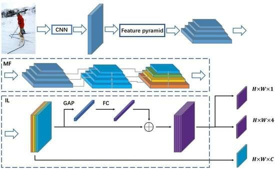
Figure 3 shows the overall structure of MFIL-FCOS, which consists of a feature extraction stage and a candidate box generation and classification stage. Backbone and FPN modules are used in the feature extraction stage. FCOS is applied to produce an ample set of candidate boxes originating from every point within the feature map, encompassing three integral branches: centerness, classification, and regression. Before performing candidate box generation and classification, the feature maps obtained through feature extraction will be inputted into the MF module for weighted integration of features at different scales. MF is designed to enhance sampling for large-scale and small-scale targets. The IL module strengthens the interaction between the regression branch and the centrality prediction branch through a special regression-prediction weight. IL is designed to achieve a more accurate regression performance.

3.2. One-Stage Anchor-Free Object Detector

Given an input image, the CNN backbone network processes it to produce feature map F i , where the value of i represents the number of feature map layers, annotated ground-truth bounding boxes indexed as B i . Each B i is defined as x 0 ( i ) , y 0 ( i ) , x 1 ( i ) , y 1 ( i ) , c ( i ) , where the pairs x 0 ( i ) , y 0 ( i ) and x 1 ( i ) , y 1 ( i ) identify the ground-truth bounding box’s upper left and lower right corners. c ( i ) tags the annotated object category, where MS-COCO and VOC datasets include 80 and 20 categories, respectively.
Each point ( x , y ) on feature map F can be mapped to a location on the input image represented by ( s 2 + x s , s 2 + y s ) . Here, s represents the total step size of the feature map scaled with respect to the input image. Our proposed anchor-free detector diverges from the anchor-based detector since the former lacks predefined anchors. In contrast, the detector regression offset represents the result of the anchor-based detector. In our regression approach, we consider the distance from pixel points on the feature map to the four bounding boxes, effectively leveraging the four distances of the regression directly as training samples, rather than as anchor boxes.
We consider a location (x,y) to be a positive sample if it lies within the ground-truth bounding box and its classification prediction c aligns with the category present in the ground truth. Conversely, we classify a location as negative if it does not lie within the ground-truth bounding box or if the classification result does not match. Our method’s regression result is a 4D vector t = ( l * , t * , r * , b * ) , where l * , t * , r * , and b * represent the distances from the location to the four boundaries. When a location (x,y) is associated with a ground-truth bounding box ( B i ), the training process’s regression distance can be expressed as:
l * = x x 0 ( i ) ,
t * = y y 0 ( i ) ,
r * = x 1 ( i ) x ,
b * = y 1 ( i ) y .

3.3. Multi-Scale Feature Fusion

Feature fusion from different scales is a crucial technique for enhancing the detection performance. Lower-level feature maps offer higher resolution and include more precise positional information. However, due to less convolution involvement, lower-layer feature maps are less semantic and more noisy. Meanwhile, higher-layer feature maps provide stronger semantic information but have a lower resolution and worse detail perception. Fusing low-level feature maps onto the high-level feature maps helps alleviate the information loss in high-dimensional feature maps to improve the classification score for small object prediction.
Object detection should concern both the deep semantic and shallow information of the image. As such, it is vital to fuse feature maps that encompass both attributes. In light of this, we propose a multi-scale feature fusion module, integrating a bottom–up feature fusion layer and an adaptive pooling layer after FPN to generate four feature maps: N 2 , N 3 , N 4 , and N 5 . Our methodology combines the layer-by-layer convolution and feature splicing of the original feature map to obtain the MF. To produce N 3 , N 2 first undergoes 3 × 3 convolution up-sampling with a stride of 1, resulting in N 2 . Subsequently, N 2 and N 2 are concatenated to achieve N 3 . N 3 , N 4 , and N 5 all adopt the above fusion method outlined in Figure 4. Each FPN feature map provides a prediction result because its receptive field is relative to network depth. While deeper feature maps have larger receptive fields, they can lose shallow semantic information. To counteract this, we perform global average pooling on the feature maps after multi-scale fusion, suppressing the overfitting and strengthening connections between categories and feature maps. Our proposed MF can be defined as follows:
N 3 = C o n c a t ( C o n v ( N 2 ) , N 2 ) ,
N 4 = C o n c a t ( C o n v ( N 3 ) , N 3 ) ,
N 5 = C o n c a t ( C o n v ( N 4 ) , N 4 ) ,
M F = A v g P o o l ( C o n c a t ( N 2 , N 3 , N 4 , N 5 ) ) .

3.4. Interactive Learning Method

When all feature points on the feature map are regressed, the quality of the resulting predicted bounding boxes is often suboptimal for locations away from the center of the object. To address this, we introduce a new centrality prediction branch alongside the regression branch. The purpose of this branch is to compute the distance from any location to the center of the predicted bounding box. Values closer to 1 indicate that the location is close to the center while values close to 0 indicate that the location is further away from the center. It is evident that bounding box regression is closely related to centrality prediction. Accordingly, for a location with bounding box regression targets of l * , t * , r * , b * , the centerness target is defined as follows:
c e n t e r n e s s * = m i n ( l * , r * ) m a x ( l * , r * ) × m i n ( t * , b * ) m a x ( t * , b * )
Object detection is often viewed as a multivariate learning challenge that jointly optimizes target classification and regression. The anchor-free detector employs a centerness estimation branch that identifies low-quality points located far from the center of the target to suppress. The independent nature of the regression branch and centerness estimation branch in existing single-stage methods may result in inconsistencies in prediction, as the key point chosen is often inconsistent in both branches. While the center point relates to the characteristics and morphology of the target, this inconsistency can lead to high centerness estimation prediction scores but inaccurate bounding box regression. To address this issue and improve the interaction between the two branches, we propose an interactive learning mechanism that enables closer collaboration and more accurate predictions. We define this mechanism as the interactive learning module. The interactive learning module is shown in Figure 5.
ω = S i g m o i d ( f c ( C o n v ( R e L U ( C o n v ( N ) ) ) ) )
I L = B m m ( N , ω )
Here, N refers to the feature map obtained after MF while Bmm represents the weighted feature map used for matrix multiplication.

3.5. Sim Box Refine

The box-refine structure used in DW [41] significantly enhances the bounding box regression ability. In this paper, a simplified method is introduced whereby a new branch is introduced for regressing the four boundary points of the bounding box, and a box refinement operation is proposed based on the predicted point offset map M R H × W × 4 to refine the bounding box. Here, (a,b) = l , t , r , b represent the distance from the object’s detected center point to its four edges. The predicted distance can then be used in fine-tuning the boundary points, and a prediction module is designed to determine the boundary point at each predicted bounding box edge as shown in Figure 6. By calculating the distances from each bounding box’s center point to its four boundaries under the feature maps of differing scales, the position of the original bounding box’s center point is adjusted using the coordinate points of the offset map as follows:
B l = ( a   + l y , b   l   + l x )
B u = ( a   t   + t y , b   + t x )
B r = ( a   + r y , b   + r   + r x )
B d = ( a   + b   + b y , b   + b x )
where B l , B u , B r , and B d denote the coordinates of the four bounding box boundary points.

3.6. Network Outputs

In the COCO dataset, our network generates a 80-dimensional vector p to predict the object category and a four-dimensional vector t for boundary box regression. By utilizing the anchor-free prediction method, the number of detection frames can be significantly reduced in comparison to the number generated using anchor-based detection algorithms. In the DIOR dataset, our network generates a 20-dimensional vector p to predict the object category and a four-dimensional vector t for boundary box regression.

3.7. Loss Function

Being an anchor-free detection algorithm, MFIL-FCOS incorporates a unique detection head onto the FPN model’s output. This detection head introduces three branches. Both the classification and centerness branches share the feature map. The branch of classification incorporates a loss function for point classification, while the branch of centerness employs a loss function for point centerness to determine whether the point represents the central region of the target. Additionally, a dedicated regression branch exists for target position regression.
MFIL-FCOS utilizes three distinct loss functions. In particular, the loss function of the point classification is implemented as follows:
L ( p x , y ) = 1 N p o s x , y L c l s ( p x , y , c x , y * )
The term L c l s denotes the focal loss. N p o s represents the count of positive samples, while p x , y signifies the classification score associated with points ( x , y ) . Additionally, c x , y * pertains to the fundamental aspect of classifying the point ( x , y ) .
The centerness loss function is defined as follows:
L ( c x , y ) = 1 N p o s x , y I c x , y * > 0 L c l s ( c x , y , c x , y * )
L c l s corresponds to the cross-entropy loss. Here, c x , y denotes the score of centerness for the point ( x , y ) , while c x , y * represents the ground truth centerness value for the same point ( x , y ) . Notably, centerness calculations are exclusively performed for positive samples.
The regression loss function is defined as follows:
L ( t x , y ) = 1 N p o s I c x , y * > 0 L r e g ( t x , y , t x , y * )
L r e g represents the IOU loss. Here, t x , y denotes the regression outcomes for the point ( x , y ) , while I c x , y * > 0 is the indicator function, taking the value of 1 for c x , y * > 0 and 0 otherwise. It is essential to note that the location regression computations are exclusively applied to positive samples.
The total loss function is defined as follows:
L ( p x , y , t x , y , c x , y ) = L ( p x , y ) + L ( t x , y ) + L ( c x , y )

4. Experiment

4.1. Datasets

Our research underwent validation using two distinct types of datasets. Initially, we utilized the COCO dataset, renowned for its diversity and comprehensive feature collection. The COCO dataset provides a vast array of annotations for everyday objects, aiding in the initial stages of acquiring distinctive features. Next, we employed the DIOR dataset, a benchmark dataset of significant scale designed for detecting targets in optical remote sensing images.

4.1.1. COCO Dataset

The COCO dataset, short for “Common Objects in Context”, is a widely used benchmark dataset in the field of computer vision and object detection. It is designed to support various computer vision tasks, such as object recognition, object detection, image segmentation, and captioning. The COCO dataset is notable for its large and diverse collection of images, making it a valuable resource for training and evaluating computer vision models.

4.1.2. DIOR Dataset

The DIOR dataset comprises 213,463 images covering 192,472 instances across 20 categories, including airports, dams, ships, and bridges. Each image measures 800 × 800 pixels, with a spatial resolution ranging from 0.5 to 30 m. The reasons for selecting DIOR for object detection lies in several factors: (1) DIOR exhibits the attributes of multi-category, multi-image, and multiple-instance scenarios; (2) Both image spatial resolution and object scales exhibit variability; (3) Due to diverse imaging conditions, encompassing different weather, seasons, and sensor sources, the dataset offers rich and varied samples; (4) The heightened intra-class diversity and diminished inter-class distinctions amplify the detection challenge and enhance the adaptability of the training model. Figure 7 visually presents the assorted samples from each category within the DIOR dataset.

4.2. Implementation Details

Data augmentation strategy. Data augmentation plays a critical role in achieving scale and rotation invariance during training. To achieve this, we apply several techniques, such as image resizing, flipping, image normalization and padding, and other augmentation methods. Specifically, we augment the size of the initial image, ensuring that the longer side is equal to or smaller than 1333 pixels, while the shorter side is equal to or smaller than 800 pixels. These methods help our models learn essential image features and prevent overfitting to the dataset.
Training details. Stochastic gradient descent (SGD) with a momentum algorithm is utilized to train all object detection models. The SGD algorithm employs an initial learning rate of 0.01 coupled with a momentum of 0.9. Under the 1× scheduler at 12 epochs, our learning rate undergoes a warm-up strategy, and its decay is triggered at epochs 8 and 11. A weight decay of 0.0001 and a training batch size of 4 are utilized. Batch normalization is utilized throughout our network’s layers. We initialized our models’ weight using publicly available ImageNet pre-trained models. Firstly, we pre-trained our model using the COCO dataset, and subsequently, fine-tuned the model on the remote sensing dataset. The model parameters are derived from the pre-training to accommodate the simple characteristics of remotely sensed images. This customized strategy guarantees the model’s competence in effectively managing diverse occlusion scenarios and intricate object characteristics inherent to remote sensing applications. A ResNet-50-based model usually requires 1.5 days to be trained on four NVIDIA 3090 GPUs.

4.3. Ablation Experiment

This study necessitates that ablation experiments are performed using the COCO dataset. These experiments are essential to confirm the method’s validity and to ascertain the significance of each module in the process.
The amount of network parameters. Table 1 presents a comparison of our network’s performance with respect to traditional network structures. Using ResNet-50 as the backbone network, our proposed architecture maintains comparable accuracies with fewer parameters, validating the effectiveness of our design.
Feature fusion methods. Detectors utilizing feature fusion hold promise in enhancing detection performance, especially for small and irregular objects. This capability stems from their capacity to integrate the semantic information from higher-level features with the image data from lower-level feature maps. In this research, we introduce a multi-scale feature fusion approach and conduct a comparative analysis against existing methods. The PaFPN model utilizes a bi-directional fusion technique from deep to shallow and then from shallow to deep, and is the first to propose a bottom–up secondary fusion model. The BiFPN model builds on this concept with a more complex bottom–up secondary fusion process. In contrast, the RFPN model utilizes a cyclic structured feature pyramid network. We propose a simpler and more efficient lightweight module, the MF module, which yields an improved accuracy and more significant performance gains for small object detection compared to these other methods. The results of a comparative analysis of our method and others are presented in Table 2.
Task interaction. Target detection is frequently formulated as a joint optimization problem in which distinct learning mechanisms for classification and localization lead to feature space distributions with differing properties. Consequently, utilizing separate branches for prediction can result in misalignment. However, these misalignments can be mitigated by enhancing the interactivity between the distinct branches. To improve this interactivity between the classification and location branches, we propose an anchor-free detector with three branches: classification, regression, and centrality prediction. We use the product of the classification score and centrality prediction score when classifying positive and negative samples. Although the classification and centrality prediction branches interact on a task-by-task basis, there is a lack of interaction between the localization and centrality prediction branches. To address this issue and enhance the network training effects, we develop a new approach to improve the interaction between the localization and centrality prediction branches. In comparison to the method proposed by TOOD, our approach is more effective, as demonstrated in Table 3.
MFIL-FCOS. In order to attribute the contribution of each component, we progressively integrated MF, IL, Sim Box Refine, and CBAM with the ResNet-50-FPN FCOS baseline, improving the detector by adding modules. The introduction of MF in the COCO dataset improves the performance from 40.4 mAP to 40.9 mAP. The introduction of IL further improves the performance from 40.9 mAP to 41.3 mAP. The use of Sim Box Refine increases the mAP by 0.1, and the results are shown in Table 4. CBAM is a lightweight general-purpose module for generating the feature map notation diagrams, spatial and channel dimension matrix multiplication and adaptive feature learning, the integration of which increases the mAP by 0.2. In the DIOR dataset, the introduction of MF improves the performance from 0.684 mAP to 0.699 mAP, and the introduction of IL improves the performance from 0.699 mAP to 0.711 mAP, and the results are shown in Table 5.

4.4. Comparison Experiment

4.4.1. Verified on COCO Dataset

Table 6 and Table 7 present a comparison between MFIL-FCOS and other one-stage detectors using the COCO dataset. Our model training follows the same resolution and 1× learning schedule as employed by the majority of other methods to ensure a fair comparison. We present results based on a single model and a single testing scale. When using the ResNet50 network, our model reaches 41.6 with the same accuracy as DRKD, and the DRKD method has a higher accuracy in some detection scenarios because of the use of knowledge distillation. On the ResNet-101 and ResNet-101-64x4d architectures, MFIL-FCOS demonstrates the outstanding performance with an AP of 46.9 and 48.4, respectively. This surpasses the performance of other one-stage detectors such as ATSS (by 3 AP) and GFL (by 2 AP). The introduction of ResNet-101-DCN results in an even larger improvement for MFIL-FCOS, relative to other detectors on this architecture. For instance, while GFL has an improvement of 2.3 AP (45.0 → 47.3 AP), MFIL-FCOS obtains an improvement of 2.6 AP (46.9 → 49.5 AP) instead. This demonstrates the remarkable efficiency of MFIL-FCOS in collaboration with deformable convolutional networks (DCN), as it dynamically adapts the spatial distribution of learned features to align with the task. It is important to note that DCN is specifically employed in the initial two layers of the head tower within MFIL-FCOS. When using other backbone networks, our method further improves the detection accuracy as the backbone network deepens. The DRKD method does not show a significant improvement in accuracy after using other backbone networks and may require the tuning optimization of the network. In summary, Table 7 clearly illustrates that MFIL-FCOS surpasses other one-stage object detection methods, achieving a result with an AP of 49.5.

4.4.2. Analysis of the Detection Results and Convergence

Figure 8 shows the examples of the object detection results produced by FCOS and the method proposed in this paper. The top of each image is FCOS and the bottom is the detection result of this paper. Our method has a higher detection score when detecting the same object and fewer misses and false detections when detecting dense scenes. We performed additional assay experiments using MFIL-FCOS and the results are shown in Figure 9.
Figure 10 shows a comparison of the convergence curves of FCOS and the method proposed in this paper during the training process. The training is performed on the COCO dataset using a training period of 12 epochs, and the other settings are kept consistent for fairness. During the training process, the convergence curve of our method is smoother and produces less fluctuation during the training process.

4.4.3. Verified on DIOR Dataset

To evaluate the efficacy of our model, we perform a comparative analysis with cutting-edge models. The analysis of the experimental data shows that our method is better than the above methods in detecting objects such as airplanes and airports, but due to the problems of uneven light and darkness in remote sensing images and the poor color differentiation of the images, the accuracy obtained is lower in detecting some of the scenes. There are differences between the different methods, such as LO-Det having a lower detection accuracy when detecting storage tanks, MFPNet having a lower detection accuracy when detecting dams, and HakwNet having a lower detection accuracy when detecting airplanes. A comprehensive analysis of Table 8 shows that our method outperforms other methods in terms of average AP 0.722. This indicates that our method has excellent overall accuracy and achieves an excellent balance between precision and recall. In addition, our method also performs well in terms of AP 0.908 for chimneys, which is significantly better than other methods. As for the AP scores for stadiums and storage tanks, our method achieves 0.891 and 0.716, respectively, showing a competitive performance.
In Figure 11, we illustrate the detection results of our proposed approach using diverse representative objects, specifically the harbor, tennis court, and track field. Distinctly colored bounding frames signify different object categories. The integration of our proposed MFIL-FCOS enhances the extraction of features, providing more comprehensive and targeted feature representations. Furthermore, the utilization of Sim Box Refine contributes to improved outcomes in box regression. This collaborative approach empowers our model to effectively handle the recognition and localization of objects across various scales, resulting in predicted bounding boxes closely aligned with the ground truth. Nevertheless, it is important to highlight that instances of misdetection and false detection predominantly occur in scenarios with small scales and indistinct boundaries.

4.5. Discussions

Limitation of MFIL-FCOS. Although our approach has achieved satisfactory results in object detection in multi-scale scenes, there has been limited exploration of the problems that arise during the detection of real objects. In addition to detecting small objects and dense scene objects, we also need to consider the occlusion problem in the detected scene and the leakage problem in low-light detection scenarios. In addition to this, we found that some complex objects also appear frequently in other tasks, such as 3D object detection and text detection, which leaves a lot of room for further exploration. Our work combines multi-scale feature integration with interactive learning to solve multi-scale detection problems in real detection scenarios. We hope to attract more researchers to focus on the problems that arise in real detection scenarios.

5. Conclusions

In this paper, we adhere to the one-stage anchor-free framework and propose a novel multi-scale feature fusion interactive learning network (MFIL-FCOS), which includes a multi-scale feature fusion module MF and an interactive learning module IL. By using the ResNet-50 backbone network, the mAP of our method in the COCO detection dataset reached 41.6, and our method achieves an accuracy of 72.2 on the DIOR remote sensing detection dataset and maintains high detection accuracy in different categories. These findings not only confirm the efficacy of our innovative approach but also highlight its substantial potential for application in tasks related to 2D object detection and remote sensing image detection. Nonetheless, it is imperative to acknowledge that additional research is necessary to tackle the complexities presented by a broader range of intricate image tasks. Our future endeavors will be focused on enhancing and extending our methodology, thereby contributing to the ongoing progress in remote sensing image detection and 2D object detection techniques.

Author Contributions

Conceptualization, methodology, writing, funding acquisition, and supervision, G.Z. and W.Y.; software, validation, and data curation, W.Y., R.H. and G.Z. All authors have read and agreed to the published version of the manuscript.

Funding

This research was supported by the National Natural Science Foundation of China (Grant number: 32271880 and 62172231); Natural Science Foundation of Jiangsu Province of China (Grant number: BK20220107).

Data Availability Statement

The COCO Dataset is available at https://cocodataset.org/home (accessed on 21 February 2014).The DIOR Dataset is available at http://www.escience.cn/people/gongcheng/DIOR.html (accessed on 17 December 2021).

Conflicts of Interest

The authors declare no conflicts of interest.

References

  1. Yurtsever, E.; Lambert, J.; Carballo, A.; Takeda, K. A survey of autonomous driving: Common practices and emerging technologies. IEEE Access 2020, 8, 58443–58469. [Google Scholar] [CrossRef]
  2. Ghafir, I.; Prenosil, V.; Svoboda, J.; Hammoudeh, M. A survey on network security monitoring systems. In Proceedings of the 2016 IEEE 4th International Conference on Future Internet of Things and Cloud Workshops (FiCloudW), Vienna, Austria, 22–24 August 2016; pp. 77–82. [Google Scholar]
  3. Evers, R.; Masters, P. The application of low-altitude near-infrared aerial photography for detecting clandestine burials using a UAV and low-cost unmodified digital camera. Forensic Sci. Int. 2018, 289, 408–418. [Google Scholar] [CrossRef]
  4. Yadav, S.S.; Jadhav, S.M. Deep convolutional neural network based medical image classification for disease diagnosis. J. Big Data 2019, 6, 113. [Google Scholar] [CrossRef]
  5. Martínez, S.S.; Ortega, J.G.; García, J.G.; García, A.S.; Estévez, E.E. An industrial vision system for surface quality inspection of transparent parts. Int. J. Adv. Manuf. Technol. 2013, 68, 1123–1136. [Google Scholar] [CrossRef]
  6. Cracknell, A.P. The development of remote sensing in the last 40 years. Int. J. Remote Sens. 2018, 39, 8387–8427. [Google Scholar] [CrossRef]
  7. Zhang, Z.; Zhang, X.; Peng, C.; Xue, X.; Sun, J. Exfuse: Enhancing feature fusion for semantic segmentation. In Proceedings of the European Conference on Computer Vision, Munich, Germany, 8–14 September 2018; pp. 269–284. [Google Scholar]
  8. Voulodimos, A.; Doulamis, N.; Doulamis, A.; Protopapadakis, E. Deep learning for computer vision: A brief review. Comput. Intell. Neurosci. 2018, 2018, 7068349. [Google Scholar] [CrossRef] [PubMed]
  9. Holloway, T.; Miller, D.; Anenberg, S.; Diao, M.; Duncan, B.; Fiore, A.M.; Henze, D.K.; Hess, J.; Kinney, P.L.; Liu, Y.; et al. Satellite monitoring for air quality and health. Annual Rev. Biomed. Data Sci. 2021, 4, 417–447. [Google Scholar] [CrossRef]
  10. Zeng, Y.; Zhang, R.; Lim, T.J. Wireless communications with unmanned aerial vehicles: Opportunities and challenges. IEEE Commun. Mag. 2016, 54, 36–42. [Google Scholar] [CrossRef]
  11. Canty, M.J. Image Analysis, Classification and Change Detection in Remote Sensing: With Algorithms for Python; CRC Press: Boca Raton, FL, USA, 2019. [Google Scholar]
  12. Toth, C.; Jóźków, G. Remote sensing platforms and sensors: A survey. ISPRS J. Photogramm. Remote Sens. 2016, 115, 22–36. [Google Scholar] [CrossRef]
  13. Grill-Spector, K.; Kushnir, T.; Edelman, S.; Avidan, G.; Itzchak, Y.; Malach, R. Differential processing of objects under various viewing conditions in the human lateral occipital complex. Neuron 1999, 24, 187–203. [Google Scholar] [CrossRef]
  14. Aziz, L.; Salam, M.S.B.H.; Sheikh, U.U.; Ayub, S. Exploring deep learning-based architecture, strategies, applications and current trends in generic object detection: A comprehensive review. IEEE Access 2020, 8, 170461–170495. [Google Scholar] [CrossRef]
  15. Yang, X.; Sun, H.; Fu, K.; Yang, J.; Sun, X.; Yan, M.; Guo, Z. Automatic ship detection in remote sensing images from google earth of complex scenes based on multiscale rotation dense feature pyramid networks. Remote Sens. 2018, 10, 132. [Google Scholar] [CrossRef]
  16. Wu, X.; Sahoo, D.; Hoi, S.C.H. Recent advances in deep learning for object detection. Neurocomputing 2020, 396, 39–64. [Google Scholar] [CrossRef]
  17. Russakovsky, O.; Deng, J.; Su, H.; Krause, J.; Satheesh, S.; Ma, S.; Fei-Fei, L. Imagenet large scale visual recognition challenge. Int. J. Comput. Vis. 2015, 115, 211–252. [Google Scholar] [CrossRef]
  18. Lin, T.Y.; Maire, M.; Belongie, S.; Hays, J.; Perona, P.; Ramanan, D.; Zitnick, C. Microsoft COCO: Common objects in context. In Proceedings of the Computer Vision–ECCV 2014: 13th European Conference, Zurich, Switzerland, 6–12 September 2014; pp. 740–755. [Google Scholar]
  19. Everingham, M.; Van Gool, L.; Williams, C.K.; Winn, J.; Zisserman, A. The pascal visual object classes (VOC) challenge. Int. J. Comput. Vis. 2010, 88, 303–338. [Google Scholar] [CrossRef]
  20. Girshick, R. Fast R-CNN. In Proceedings of the IEEE International Conference on Computer Vision, Santiago, Chile, 7–13 December 2015; pp. 1440–1448. [Google Scholar]
  21. Redmon, J.; Farhadi, A. Yolov3: An incremental improvement. arXiv 2018, arXiv:1804.02767. [Google Scholar]
  22. Tian, Z.; Shen, C.; Chen, H.; He, T. FCOS: Fully convolutional one-stage object detection. In Proceedings of the IEEE/CVF International Conference on Computer Vision, Seoul, Republic of Korea, 27 October–2 November 2019; pp. 9627–9636. [Google Scholar]
  23. Duan, K.; Bai, S.; Xie, L.; Qi, H.; Huang, Q.; Tian, Q. Centernet: Keypoint triplets for object detection. In Proceedings of the IEEE/CVF International Conference on Computer Vision, Seoul, Republic of Korea, 27 October–2 November 2019; pp. 6569–6578. [Google Scholar]
  24. Law, H.; Deng, J. Cornernet: Detecting objects as paired keypoints. In Proceedings of the European Conference on Computer Vision, Munich, Germany, 8–14 September 2018; pp. 734–750. [Google Scholar]
  25. Zhou, X.; Zhuo, J.; Krahenbuhl, P. Bottom-up object detection by grouping extreme and center points. In Proceedings of the IEEE/CVF Conference on Computer Vision and Pattern Recognition, Long Beach, CA, USA, 15–20 June 2019; pp. 850–859. [Google Scholar]
  26. Yu, D.; Ji, S. A New Spatial-Oriented Object Detection Framework for Remote Sensing Images. IEEE Trans. Geosci. Remote Sens. 2021, 60, 3127232. [Google Scholar] [CrossRef]
  27. Zhang, T.; Zhang, X. Foreground Refinement Network for Rotated Object Detection in Remote Sensing Images. IEEE Trans. Geosci. Remote Sens. 2021, 60, 5610013. [Google Scholar] [CrossRef]
  28. Wang, J.; He, X. Multi-Size Object Detection in Large Scene Remote Sensing Images Under Dual Attention Mechanism. IEEE Access 2022, 10, 8021–8035. [Google Scholar] [CrossRef]
  29. Bai, J.; Ren, J. Object Detection in Large-Scale Remote-Sensing Images Based on Time-Frequency Analysis and Feature Optimization. IEEE Trans. Geosci. Remote Sens. 2021, 60, 5405316. [Google Scholar] [CrossRef]
  30. Cheng, B.; Li, Z. Target detection in remote sensing image based on object-and-scene context constrained CNN. IEEE Geosci. Remote Sens. Lett. 2021, 19, 8013705. [Google Scholar] [CrossRef]
  31. Li, Y.; Huang, Q.; Pei, X.; Chen, Y. Cross-layer attention network for small object detection in remote sensing imagery. IEEE J. Sel. Top. Appl. Earth Obs. Remote Sens. 2020, 14, 2148–2161. [Google Scholar] [CrossRef]
  32. Zhang, X.; Gong, Z.; Guo, H.; Liu, X.; Ding, L.; Zhu, K.; Wang, J. Adaptive Adjacent Layer Feature Fusion for Object Detection in Remote Sensing Images. Remote Sens. 2023, 15, 4224. [Google Scholar] [CrossRef]
  33. Csurka, G.; Dance, C.; Fan, L.; Willamowski, J.; Bray, C. Visual categorization with bags of keypoints. Workshop Stat. Learn. Comput. Vis. 2004, 1, 1–2. [Google Scholar]
  34. Li, K.; Zou, C.; Bu, S.; Liang, Y.; Zhang, J.; Gong, M. Multi-modal feature fusion for geographic image annotation. Pattern Recognit. 2018, 73, 1–14. [Google Scholar] [CrossRef]
  35. Ye, T.; Zhang, X.; Zhang, Y.; Liu, J. Railway traffic object detection using differential feature fusion convolution neural network. IEEE Trans. Intell. Transp. Syst. 2020, 22, 1375–1387. [Google Scholar] [CrossRef]
  36. Wang, F.; Peng, J.; Li, Y. Hypergraph based feature fusion for 3-D object retrieval. Neurocomputing 2015, 151, 612–619. [Google Scholar] [CrossRef]
  37. Haussmann, E.; Fenzi, M.; Chitta, K.; Ivanecky, J.; Xu, H.; Roy, D.; Alvarez, J.M. Scalable active learning for object detection. In Proceedings of the 2020 IEEE Intelligent Vehicles Symposium, Las Vegas, NV, USA, 19 October–13 November 2020; pp. 1430–1435. [Google Scholar]
  38. Yao, A.; Gall, J.; Leistner, C.; Van Gool, L. Interactive object detection. In Proceedings of the 2012 IEEE Conference on Computer Vision and Pattern Recognition, Providence, RI, USA, 16–21 June 2012; pp. 3242–3249. [Google Scholar]
  39. Li, Y.; Huang, D.; Qin, D.; Wang, L.; Gong, B. Improving object detection with selective self-supervised self-training. In Proceedings of the European Conference on Computer Vision, Glasgow, UK, 23–28 August 2020; pp. 589–607. [Google Scholar]
  40. Ball, J.E.; Anderson, D.T.; Chan, C.S. Comprehensive survey of deep learning in remote sensing: Theories, tools, and challenges for the community. Remote Sens. 2017, 11, 042609. [Google Scholar] [CrossRef]
  41. Li, S.; He, C.; Li, R.; Zhang, L. A dual weighting label assignment scheme for object detection. In Proceedings of the IEEE/CVF Conference on Computer Vision and Pattern Recognition, New Orleans, LA, USA, 18–24 June 2022; pp. 9387–9396. [Google Scholar]
  42. Kong, T.; Sun, F.; Liu, H.; Jiang, Y.; Li, L.; Shi, J. Foveabox: Beyound anchor-based object detection. IEEE Trans. Image Process. 2020, 29, 7389–7398. [Google Scholar] [CrossRef]
  43. Zhang, S.; Chi, C.; Yao, Y.; Lei, Z.; Li, S.Z. Bridging the gap between anchor-based and anchor-free detection via adaptive training sample selection. In Proceedings of the IEEE/CVF Conference on Computer Vision and Pattern Recognition, Seattle, WA, USA, 13–19 June 2020; pp. 9759–9768. [Google Scholar]
  44. Kim, K.; Lee, H.S. Probabilistic anchor assignment with iou prediction for object detection. In Proceedings of the Computer Vision—ECCV 2020: 16th European Conference, Glasgow, UK, 23–28 August 2020; pp. 355–371. [Google Scholar]
  45. Ge, Z.; Liu, S.; Li, Z.; Yoshie, O.; Sun, J. OTA: Optimal transport assignment for object detection. In Proceedings of the IEEE/CVF Conference on Computer Vision and Pattern Recognition, Nashville, TN, USA, 20–25 June 2021; pp. 303–312. [Google Scholar]
  46. Zhu, B.; Wang, J.; Jiang, Z.; Zong, F.; Liu, S.; Li, Z.; Sun, J. Autoassign: Differentiable label assignment for dense object detection. arXiv 2007, arXiv:2007.03496. [Google Scholar]
  47. Ke, W.; Zhang, T.; Huang, Z.; Ye, Q.; Liu, J.; Huang, D. Multiple anchor learning for visual object detection. In Proceedings of the IEEE/CVF Conference on Computer Vision and Pattern Recognition, Seattle, WA, USA, 13–19 June 2020; pp. 10206–10215. [Google Scholar]
  48. Li, X.; Wang, W.; Wu, L.; Chen, S.; Hu, X.; Li, J.; Yang, J. Generalized focal loss: Learning qualified and distributed bounding boxes for dense object detection. Adv. Neural Inf. Process. Syst. 2020, 33, 21002–21012. [Google Scholar]
  49. Zhang, H.; Wang, Y.; Dayoub, F.; Sunderhauf, N. Varifocalnet: An IoU-aware dense object detector. In Proceedings of the IEEE/CVF Conference on Computer Vision and Pattern Recognition, Nashville, TN, USA, 20–25 June 2021; pp. 8514–8523. [Google Scholar]
  50. Gao, Z.; Wang, L.; Wu, G. Mutual supervision for dense object detection. In Proceedings of the IEEE/CVF International Conference on Computer Vision, Nashville, TN, USA, 20–25 June 2021; pp. 3641–3650. [Google Scholar]
  51. Feng, C.; Zhong, Y.; Gao, Y.; Scott, M.R.; Huang, W. TOOD: Task-aligned one-stage object detection. In Proceedings of the 2021 IEEE/CVF International Conference on Computer Vision, Nashville, TN, USA, 20–25 June 2021; pp. 3490–3499. [Google Scholar]
  52. Ni, Z.; Yang, F.; Wen, S.; Zhang, G. Dual Relation Knowledge Distillation for Object Detection. arXiv 2023, arXiv:2302.05637. [Google Scholar]
  53. Ma, Y.; Liu, S.; Li, Z.; Sun, J. Iqdet: Instance-wise quality distribution sampling for object detection. In Proceedings of the IEEE/CVF Conference on Computer Vision and Pattern Recognition, Nashville, TN, USA, 19–25 June 2021; pp. 1717–1725. [Google Scholar]
  54. Liu, W.; Anguelov, D.; Erhan, D.; Szegedy, C.; Reed, S.; Fu, C.-Y.; Berg, A.C. SSD: Single shot multibox detector. In Proceedings of the ECCV 2016: 14th European Conference, Amsterdam, The Netherlands, 11–14 October 2016; pp. 21–37. [Google Scholar]
  55. Huang, Z.; Li, W.; Xia, X.G.; Wu, X.; Cai, Z.; Tao, R. A novel nonlocal-aware pyramid and multiscale multitask refinement detector for object detection in remote sensing images. IEEE Trans. Geosci. Remote Sens. 2021, 60, 5601920. [Google Scholar] [CrossRef]
  56. Bochkovskiy, A.; Wang, C.Y.; Liao, H.Y.M. Yolov4: Optimal speed and accuracy of object detection. arXiv 2020, arXiv:2004.10934. [Google Scholar]
  57. Tan, M.; Pang, R.; Le, Q.V. Efficientdet: Scalable and efficient object detection. In Proceedings of the IEEE/CVF Conference on Computer Vision and Pattern Recognition, Seattle, WA, USA, 14–19 June 2020; pp. 10781–10790. [Google Scholar]
  58. Ye, Y.; Ren, X.; Zhu, B.; Tang, T.; Tan, X.; Gui, Y.; Yao, Q. An adaptive attention fusion mechanism convolutional network for object detection in remote sensing images. Remote Sens. 2022, 14, 516. [Google Scholar] [CrossRef]
  59. Lei, T.; Zhang, D.; Wang, R.; Li, S.; Zhang, W.; Nandi, A.K. MFP-Net: Multi-scale feature pyramid network for crowd counting. IET Image Process. 2021, 15, 3522–3533. [Google Scholar] [CrossRef]
  60. Nakanishi, H.; Suzuki, M.; Matsuo, Y. HAWK-Net: Hierarchical Attention Weighted Top-K Network for High-resolution Image Classification. J. Inf. Process. 2023, 31, 851–859. [Google Scholar] [CrossRef]
Figure 1. Examples of the multi-scale scene challenges. The image on the left shows small-scale objects that are densely distributed and difficult to detect. The right image is a large-scale object that occupies a large number of pixels.
Remotesensing 16 00936 g001
Figure 2. The network architecture of FCOS. C3, C4, and C5 were from the backbone network. For final predictions, feature levels P3–P7 were employed. The dimensions H × W correspond to the height and width of the feature map. The ‘/s’ notation, where ‘s’ ranges from 8 to 128, signifies the downsampling rate from the input image.
Remotesensing 16 00936 g002
Figure 3. The network architecture of MFIL-FCOS. MFIL-FCOS is improved based on the FCOS network; MF is the multi-scale feature fusion module; and IL is the interactive learning module.
Remotesensing 16 00936 g003
Figure 4. The architecture of the MF module. When fusing deep feature maps upwards, a 3 × 3 convolution is used along with a 2× upsampling operation. When fusing down shallow feature maps, a 1 × 1 convolution along with a 2× downsampling operation. The final feature map is output after feature concatenation.
Remotesensing 16 00936 g004
Figure 5. The architecture of the IL module. GAP denotes the global average pooling of the feature map and FC is the output of features using a fully connected layer. The output feature maps are used for centerness prediction and regression branching.
Remotesensing 16 00936 g005
Figure 6. Illustration of Sim Box Refine. A coarse bounding box (orange box) at the location is first generated by predicting the four distances = { l , t , r , b } . Four boundary points (orange points) are then predicted with respect to the four side points (green points). Finally, a finer bounding box (green box) is generated by aggregating the prediction results of the four boundary points.
Remotesensing 16 00936 g006
Figure 7. Image samples of 20 categories from the DIOR dataset. The list comprises 20 distinct object classes, namely airplane, airport, baseball field, basketball court, bridge, chimney, dam, expressway service area, expressway toll station, harbor, golf course, ground track field, overpass, ship, stadium, storage tank, tennis court, train station, vehicle, and windmill.
Remotesensing 16 00936 g007
Figure 8. Examples of the detection results of FCOS versus MFIL-FCOS. Both models implement a ResNet-50 backbone architecture for object detection, trained using the COCO dataset. The detection results of FCOS and MFIL-FCOS are presented above and below, respectively. It is evident that MFIL-FCOS outperforms FCOS in detecting larger objects, and it can identify denser and smaller objects that FCOS fails to detect.
Remotesensing 16 00936 g008
Figure 9. Examples of MFIL-FCOS detection results on the COCO dataset. These results demonstrate that MFIL-FCOS performs effectively in diverse scenes, including occluded scenes, dense scenes, and multi-scale scenes.
Remotesensing 16 00936 g009
Figure 10. Convergence curves. MFIL-FCOS accelerates the training process for FCOS variants. The x axis corresponds to epochs and the y axis corresponds to the mAP evaluated on COCO dataset.
Remotesensing 16 00936 g010
Figure 11. Examples of the MFIL-FCOS detection results on the DIOR dataset. It can be seen that, for some small-scale objects such as ships, MFIL-FCOS is able to detect them well.
Remotesensing 16 00936 g011
Table 1. Comparison of parameters between MFIL-FCOS and other detection methods. We statistically analyze the total number of parameters for these different methods.
MethodParams
RetianNet37.41 M
DETR41.3 M
YOLOF43.88 M
MFIL-FCOS38.83 M
Table 2. Comparison of MF with other feature fusion methods. + indicates the increase in the number of method parameters when the module is added compared to the original.
MethodParamsGFLOPsmAPAR
PAFPN+6.885 M24.840.7820.937
BiFPN+4.66 M38.1260.7760.929
RFPN+3.608 M17.7290.7820.932
MF+2.361 M15.1190.7870.933
Table 3. Comparison of MFIL-FCOS and TOOD on different interactive learning strategies. We conduct experiments using two interaction learning strategies: cls + reg, which applies interaction learning to the classification and localization branches, and reg + center, which applies interaction learning to the localization and centrality prediction branches.
MethodTask InteractionBackboneAPAP50AP75APSAPMAPL
TOOD(cls + reg)ResNet-5040.959.344.3
MFIL-FCOS(reg + center)ResNet-5041.659.945.0
TOOD(cls + reg)ResNet-10146.764.650.728.949.657.0
MFIL-FCOS(reg + center)ResNet-10146.965.350.527.849.958.9
Table 4. MFIL-FCOS modular ablation experiments on the COCO dataset. × indicates that we do not add the module to the experiment, and ✓ indicates that we add the module to the experiment. Bold indicates the best performance.
MethodMFILSim Box RefineCBAMmAP
Baseline××××40.4
×××40.9
××41.3
×41.4
41 . 6
Table 5. MFIL-FCOS modular ablation experiments on the DIOR dataset. × indicates that we do not add the module to the experiment, and ✓ indicates that we add the module to the experiment. Bold indicates the best performance.
MethodMFILSim Box RefineCBAMmAP
Baseline××××0.684
×××0.699
××0.711
×0.716
0 . 722
Table 6. Results for our MFIL-FCOS and other detection models. These models are trained on the COCO dataset with the ResNet50 backbone and the training period is 12 epochs. Bold indicates that the best performance is achieved in that metric.
MethodAPAP50AP75Reference
FoveaBox [42]36.455.838.8-
FCOS [22]38.657.441.4ICCV19
ATSS [43]39.257.442.4CVPR20
PAA [44]40.458.443.9ECCV20
OTA [45]40.758.444.3CVPR21
AutoAssign [46]40.459.643.7-
NoisyAnchor38.056.940.6CVPR20
MAL [47]39.258.042.3CVPR20
GFL [48]39.958.543.0NeurIPS20
VFL [49]40.258.244.0CVPR21
FCOS + GFLv240.658.243.9CVPR21
ATSS + GFLv241.158.844.9CVPR21
Musu [50]40.658.944.3ICCV21
TOOD [51]40.358.543.8ICCV21
DW [41]41.559.845.0CVPR22
DRKD [52] 41 . 6 59.7 45 . 3 IJCAI23
MFIL-FCOS (ours) 41 . 6 59 . 9 45 . 0 -
Table 7. Results for our MFIL-FCOS and other detection models under the same setting. ResNet101-DCN indicates the use of deformable convolution in the experiment. ResNet-101 (64x4d) indicates that, in the residual module, the convolution layer is a grouped convolution with 64 groups of 4 channels each. Bold indicates the best performance.
MethodBackboneAPAP50AP75APSAPMAPLReference
FCOS [22]ResNet-10141.560.745.024.444.851.6ICCV19
ATSS [43]ResNet-10143.662.147.426.147.053.6CVPR20
PAA [44]ResNet-10144.863.348.726.548.856.3ECCV20
GFL [48]ResNet-10145.063.748.927.248.854.5NeurIPS20
IQDet [53]ResNet-10145.163.449.326.745.556.6CVPR19
Musu [50]ResNet-10144.863.249.126.247.956.4ICCV21
AutoAssign [46]ResNet-10144.564.348.425.947.455.0-
VFL [49]ResNet-10144.964.148.927.149.458.5CVPR21
DW [41]ResNet-10146.665.150.327.549.658.6CVPR22
DRKD [52]ResNet-10146.765.150.127.649.658.7IJCAI23
MFIL-FCOS (ours)ResNet-101 46 . 9 65 . 3 50 . 5 27 . 8 49 . 9 58 . 9 -
ATSS [43]ResNet-101-DCN46.364.750.427.749.858.4CVPR20
PAA [44]ResNet-101-DCN47.465.751.627.951.360.6ECCV20
GFL [48]ResNet-101-DCN47.366.351.428.051.159.2NeurIPS20
Musu [50]ResNet-101-DCN47.465.051.827.850.560.0ICCV21
VFL [49]ResNet-101-DCN48.567.452.929.152.261.9CVPR21
DW [41]ResNet-101-DCN49.3 67 . 7 53.329.352.263.5CVPR22
DRKD [52]ResNet-101-DCN49.367.553.329.452.2 63 . 6 IJCAI23
MFIL-FCOS (ours)ResNet-101-DCN 49 . 5 67 . 7 53 . 5 29 . 5 52 . 4 63 . 6 -
ATSS [43]ResNet-101-64x4d45.664.649.728.548.955.6CVPR20
PAA [44]ResNet-101-64x4d46.665.650.828.850.457.9ECCV20
GFL [48]ResNet-101-64x4d46.065.150.128.249.656.0NeurIPS20
OTA [45]ResNet-101-64x4d47.065.851.129.250.457.9CVPR21
DW [41]ResNet-101-64x4d48.267.1 52 . 2 29.651.260.8CVPR22
DRKD [52]ResNet-101-64x4d48.066.952.029.551.160.5IJCAI23
MFIL-FCOS (ours)ResNet-101-64x4d 48 . 4 67 . 2 52 . 2 29 . 8 51 . 3 60 . 9 -
Table 8. Comparison with other methods on the DIOR dataset. Our training period is 12 epochs. Other settings are kept consistent in order to ensure the fairness of the experiment. Bold indicates that the best performance is achieved in that metric.
ClassSSD [54]LO-Det [55]YOLOv4 [56]Efficient Det [57]AAFM [58]MFPNet [59]HakwNet [60]MFIL-FCOS (Ours)
airplane0.6680.7260.6820.6880.7160.7660.657 0 . 909
airport0.6870.6500.7020.7420.7510.8340.842 0 . 907
baseball field0.7040.7670.7590.8030.8260.8060.761 0 . 907
basketball court0.7630.8460.8060.7780.8100.821 0 . 874 0.800
bridge0.3340.3340.4140.4030.4590.443 0 . 453 0.411
chimney0.6680.7370.7130.6830.7040.7560.790 0 . 908
dam0.5650.5680.6030.6430.6900.6850.645 0 . 730
expressway-service area0.6480.7580.7760.8160.8320.8590.828 0 . 867
expressway-toll station0.5740.5750.6630.6710.6820.639 0 . 724 0.719
golf field0.6620.6620.7550.7750.7840.7730.825 0 . 831
ground track field0.6750.6800.7550.7950.8080.7720.747 0 . 805
harbor0.3950.6090.4720.4680.4830.6210.502 0 . 668
overpass0.4950.5150.5600.5760.5980.5880.596 0 . 672
ship0.6970.8860.7340.7460.7680.772 0 . 897 0.753
stadium0.6600.6800.6960.8070.8100.7680.660 0 . 891
storage tank0.4960.6430.5610.5320.5660.6030.708 0 . 716
tennis court0.7710.8620.8330.8400.8560.864 0 . 872 0.854
train station0.5380.4750.5830.5790.605 0 . 645 0.6140.603
vehicle0.3750.4240.4430.4300.4560.415 0 . 528 0.317
windmill0.6740.7670.7570.7590.7650.802 0 . 882 0.710
mAP0.6020.6580.6730.6770.6980.7120.720 0 . 722
Disclaimer/Publisher’s Note: The statements, opinions and data contained in all publications are solely those of the individual author(s) and contributor(s) and not of MDPI and/or the editor(s). MDPI and/or the editor(s) disclaim responsibility for any injury to people or property resulting from any ideas, methods, instructions or products referred to in the content.

