
SAM-Induced Pseudo Fully Supervised Learning for Weakly Supervised Object Detection in Remote Sensing Images


College of Electrical and Information Engineering, Zhengzhou University of Light Industry, Zhengzhou 450002, China
*
Author to whom correspondence should be addressed.
Remote Sens. 2024, 16(9), 1532; https://doi.org/10.3390/rs16091532
Submission received: 12 March 2024
/
Revised: 19 April 2024
/
Accepted: 23 April 2024
/
Published: 26 April 2024
(This article belongs to the Special Issue Object Detection and Information Extraction Based on Remote Sensing Imagery)
Abstract
:Weakly supervised object detection (WSOD) in remote sensing images (RSIs) aims to detect high-value targets by solely utilizing image-level category labels; however, two problems have not been well addressed by existing methods. Firstly, the seed instances (SIs) are mined solely relying on the category score (CS) of each proposal, which is inclined to concentrate on the most salient parts of the object; furthermore, they are unreliable because the robustness of the CS is not sufficient due to the fact that the inter-category similarity and intra-category diversity are more serious in RSIs. Secondly, the localization accuracy is limited by the proposals generated by the selective search or edge box algorithm. To address the first problem, a segment anything model (SAM)-induced seed instance-mining (SSIM) module is proposed, which mines the SIs according to the object quality score, which indicates the comprehensive characteristic of the category and the completeness of the object. To handle the second problem, a SAM-based pseudo-ground truth-mining (SPGTM) module is proposed to mine the pseudo-ground truth (PGT) instances, for which the localization is more accurate than traditional proposals by fully making use of the advantages of SAM, and the object-detection heads are trained by the PGT instances in a fully supervised manner. The ablation studies show the effectiveness of the SSIM and SPGTM modules. Comprehensive comparisons with 15 WSOD methods demonstrate the superiority of our method on two RSI datasets.
1. Introduction
Compared with fully supervised object detection (FSOD) [1,2,3,4,5,6,7,8], the major advantage of weakly supervised object detection (WSOD) is that only image-level category annotations are necessary for training the WSOD model. Considering the low cost of data labeling, WSOD has been widely researched in recent years [9,10,11,12,13,14,15,16,17] and has been applied in scene classification [18,19], disaster detection [20,21], military [22,23], and other applications [24,25,26,27,28,29].
Weakly supervised deep detection networks (WSDDNs) [30] firstly combined deep learning with multiple instance learning (MIL) [30,31,32,33,34], and online instance classifier refinement (OICR) [31] introduced the instance classifier refinement (ICR) branch based on the WSDDN. OICR has been adopted as the baseline framework by many WSOD methods, and its process is briefly described as follows. Firstly, generate proposals through selective search (SS) [35], and import them into the backbone network to attain their features. Then, the instance-level category score (CS) of each proposal is obtained through MIL learning. Finally, the CSs are continuously optimized by several ICR branches, where the positive samples of each ICR branch include the seed instance (SI) and its neighbor instance, and the proposal with the highest CS predicted by the previous ICR branch is defined as the SI.
So far, there are still two problems that have not been well solved in the above baseline framework. For the first problem, the SIs that are mined solely relying on the CS are unreliable. On the one hand, existing methods usually select instances with high CSs as the SIs [31,32,36,37,38,39]; however, these instances usually focus on the most salient parts, rather than the whole object. On the other hand, compared with natural scene images (NSIs), remote sensing images (RSIs) have a more complex background; consequently, the reliability of the predicted CSs and SIs mined by the CSs is insufficient.
For the second problem, the localization capability of existing methods [34,40,41,42] is restricted by the proposals generated by the SS or edge boxes (EBs) [43]. As a matter of fact, most of the WSOD methods focus on improving the CS of each proposal, and the localization of each proposal is not changed. Although recent works added a regression branch for each ICR branch, where the SIs are used as the pseudo-ground truth (PGT) of each regression branch, the SIs are selected from the proposals; in other words, the localization of the SIs is still determined by the SS (EB). Considering that the SS (EB) is an early method in which the deep learning technique is not applied, its localization capability is limited, which has become a bottleneck of object localization for WSOD.
In order to address the aforementioned problems, a novel segment anything model (SAM)-induced pseudo-fully supervised learning (SPFS) model is proposed for WSOD in RSIs. Specifically, to overcome the first problem, as shown in Figure 1, a SAM-induced seed instance-mining (SSIM) module is proposed. First of all, the SAM-induced bounding boxes (SAMBs) are generated from the segmentation map inferred by SAM, where each SAMB tightly encloses one segment. Afterwards, the SAMBs are utilized to calculate the object completeness score (OCS) of each proposal. Finally, the OCS is integrated with the CS to obtain the object quality score (OQS), which is more reliable than the CS and can indicate the comprehensive characteristic of the object category and the object completeness, and the OQS is used to mine the SIs.
To overcome the second issue, a SAM-based pseudo-ground truth-mining (SPGTM) strategy is proposed for training the pseudo-fully supervised object-detection (PFSOD) head. The PGT instances of each PFSOD head are mined from the SAMBs according to the spatial relationship between the SAMBs and SIs of each ICR branch; consequently, the localization of mined PGT instances is more accurate than traditional proposals by fully making use of the advantages of SAM.
The main contributions of our method are as follows:
- An SSIM module is proposed to address the issue of the SIs that are mined solely depending on the CS being unreliable. The SSIM module mines the SIs according to the OQS, which can indicate the comprehensive characteristic of the object category and the object completeness;
- An SPGTM strategy is proposed to break the bottleneck of object localization brought by the SS or EB. The SPGTM strategy is utilized to mine PGT instances, for which the localization is more accurate than traditional proposals by fully making use of the advantages of SAM, and then, the PFSOD head is trained by using the PGT instances;
- To our best knowledge, this is the first attempt to build a WSOD model by using the vision foundation model. It is worth noting that our SPFS model gives a unified solution of how to improve the localization capability of the WSOD model by using the segmentation technique; in other words, SAM is not the only choice for segmentation, and it can be replaced by better segmentation models in the future.
2. Related Works
To handle the problem that a single image contains multiple objects, many methods have changed from selecting the highest score of proposals to the local highest score for mining more SIs. On the one hand, some classical methods select the highest score of proposals as the SI. For example, Tang et al. [31] proposed an OICR model, which selected the highest prediction CS of the proposals as the SI, and then, the SI with its neighboring instances were used to train the WSOD model. Wu et al. [40] proposed to combine bottom-up aggregated attention (BUAA) and a phase-aware loss to select the highest CS of the proposals as the SI. Other similar works include [34,44], etc.
On the other hand, some improved methods select the local highest score of the proposals as the SIs. For example, Tang et al. [37] proposed a proposal-cluster-learning (PCL) scheme, which divided the prediction CS of the proposals into multiple clusters to mine the SIs for training the WSOD model. Ren et al. [32] proposed a multiple instance self-training (MIST) strategy, which selected the top prediction CSs as the candidate SIs, and the final SIs were determined by using the local NMS strategy among the candidate SIs. The mining high-quality pseudo-instance soft labels (MHQ-PSL) scheme [9] uses the proposal quality score to mine PGT instances and assign soft labels to each instance. Qian et al. [10] proposed an objectness score to mine SIs and incorporated the difficulty evaluation score into the training loss. The semantic segmentation-guided pseudo-label mining and instance re-detection (SGPLM-IR) method [11] proposes a class-specific object confidence score to mine PGT instances and an instance re-detection module to improve localization accuracy.
3. Basic WSOD Framework
3.1. Weakly Supervised Deep Detection Network
Currently, most of the WSOD methods use the OICR as the basic framework, which is constructed on the basis of the WSDDN, which is used to infer the initial CS of each proposal. Then, the OICR uses K ICR branches to continuously refine the CSs. The final detection results are obtained through non-maximum suppression (NMS) [45,46,47,48,49] in terms of the CSs.
Specifically, as shown in Figure 1, firstly, a series of proposals of the input image, denoted as , is generated through the SS, where denotes the amount of proposals. Secondly, the corresponding feature map is obtained by importing the image into the backbone, and then, the proposal is imported to the region of interest (RoI) pooling and two fully connected (FC) layers in the proper sequence to acquire the corresponding feature vector. Thirdly, the classification and detection score matrices are acquired by inputting the feature vectors into two parallel streams. The final score matrix, denoted as , is obtained through the elementwise product of two matrices. The final image-level prediction score of category v, denoted as , can be attained by the following equation:
where V denotes the quantity of the category and denotes the element in the vth row and jth column of Z. At this point, the WSDDN can be optimized by the following loss:
where represents the loss function of the WSDDN and represents the image-level label of category v; if the image contains category v, and otherwise, .
3.2. Online Instance Classifier Refinement
Fourthly, the CS matrices, denoted as , are attained by inputting the feature vectors of all proposals into the kth ICR stream, where and the category represents the background. The index of the proposal with the highest CS of category v in the ICR stream is denoted as , and then, is defined as the SI of category v in the kth ICR stream. The assemble of positive samples of category v in the kth ICR stream, denoted as , consists of and its neighbor proposals. Finally, the loss function of the ICR branch is formulated as follows:
where represents the CS of for category v in the kth ICR stream, denotes the weight of , and represents the CS of for category v in the ()th ICR stream; if , and otherwise, .
3.3. Bounding Box Regression
Similar to recent WSOD methods [10,50], a bounding box regression (BBR) branch is attached to each ICR branch to improve the localization capability. The loss function of the kth BBR stream is defined as follows:
where denotes the cardinality of , denotes the smooth L1 loss function [1], and and denote the predicted and target localization offsets of the ith positive sample of category v in the kth BBR branch, respectively.
4. Proposed Method
4.1. Overview
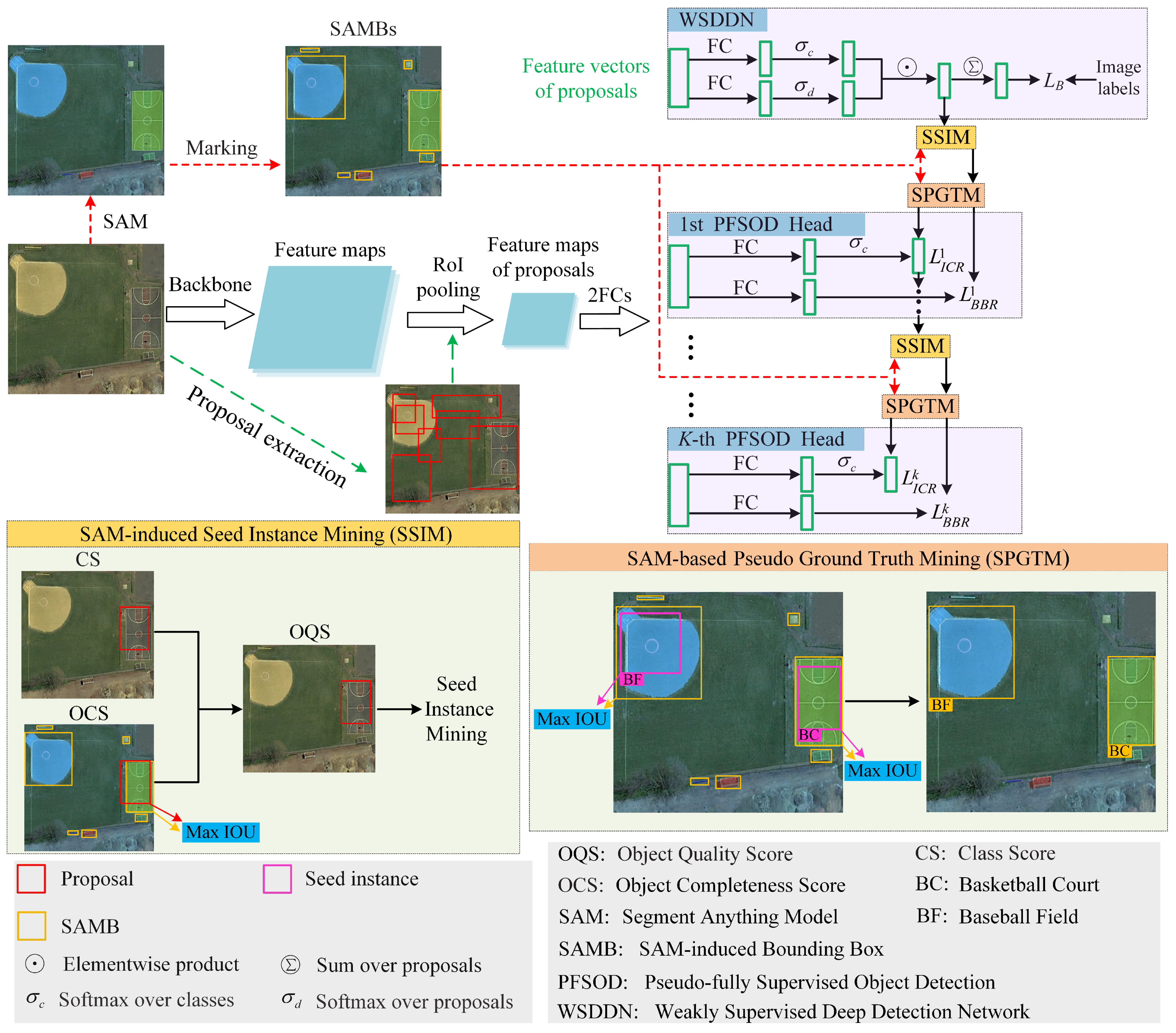
As shown in Figure 1 and Section 3, our SPFS model utilizes the “OICR+BBR” as the basic WSOD framework, and the proposed SSIM and SPGTM modules are incorporated into it. Firstly, the RSI is fed into the backbone to obtain its feature maps, and the SS algorithm is used to extract the proposals from the RSI. Secondly, the above proposals are projected onto the feature maps, and their feature maps with a fixed size are generated through the RoI pooling operation, then the feature maps of the proposals are fed into two FC layers to extract the feature vector of each proposal. Thirdly, the feature vectors of all proposals are fed into the WSDDN trained by image-level labels to acquire the CS of all proposals, and the related details can be seen in Section 3.1. Fourthly, the segmentation map of the RSI is generated by using SAM (the related details can be seen in Section 4.2), and then, the rectangles are marked on it to obtain the SAMBs. Fifthly, the CSs of all proposals and SAMBs are fed into the SSIM module to mine high-quality SIs, and the related details can be seen in Section 4.3. Sixthly, the SIs and SAMBs are fed into the SPGTM module to obtain the PGT instances of the RSI, and the related details can be seen in Section 4.4. Seventhly, the feature vectors of all proposals are fed into the first PFSOD head trained by the above PGT instances to refine the CSs of all proposals. Steps 5∼step 7 are repeated K-times to accomplish the training of K PFSOD heads, and the related details can be seen in Section 4.5. Finally, the K trained PFSOD heads are jointly used to infer the detection results.
4.2. Segment Anything Model
SAM [51] is a proposed vision foundation model based on deep learning technology. Over eleven million images with over one billion masks are used to train SAM through a multi-stage learning scheme; thus, SAM can learn more complex image features and the morphology of foreground objects. Compared to traditional image-segmentation methods [52,53,54], SAM can precisely segment various objects with any shape and category in more complex scenarios, such as RSIs. Furthermore, SAM has an excellent capability in terms of being real time and in terms of accuracy, whether on static images or dynamic videos, which provides powerful support for various practical applications.
4.3. SAM-Induced Seed Instance Mining
First of all, the segmentation map of the input RSI is inferred by SAM, which is a powerful universal segmentation model, as shown in the top-left corner of Figure 1; each segment is visualized with different colors. Secondly, the SAMB of each segment is marked according to the coordinates of the four vertices of each segment; consequently, each segment is tightly enclosed by its SAMB.
Thirdly, the OCS of proposal , denoted as , is calculated through the following equation:
where B denotes the assemble of all SAMBs, denotes the number of SAMBs, denotes the nth SAMB in B, denotes the IoU between and , and denotes the operation of taking the maximum value. Equation (5) is used to measure the completeness by which each proposal covers the foreground object by using the advantages of SAM, which can precisely and fully cover each object.
Fourthly, the OQS of for category v in the kth ICR branch, denoted as , is calculated through the following equation:
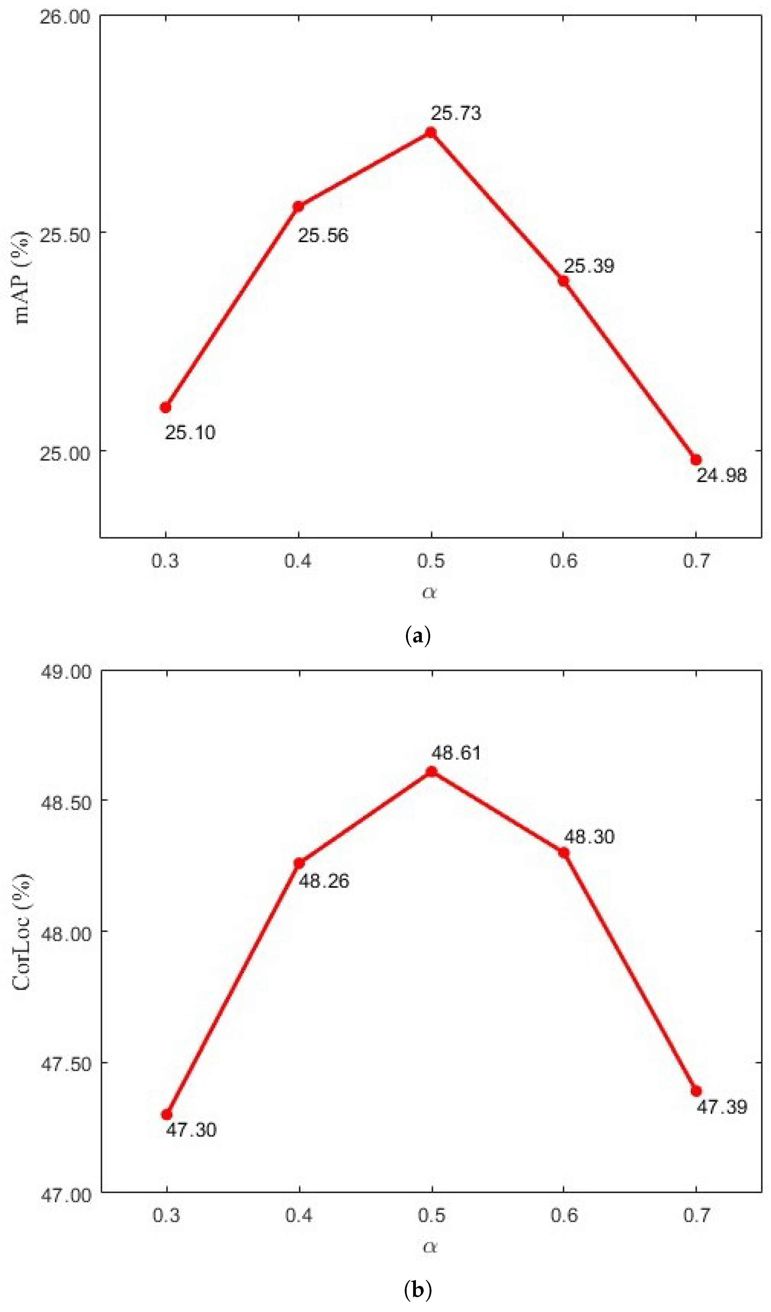
where is used to adjust the relative weight between and As shown in Equation (6), the OQS of each proposal is composed of the CS and OCS; consequently, the SIs mined through the OQS have accurate category information and can cover the objects as much as possible. Inspired by MHQ-PSLs [9] and SGPLM-IR [11], is defined as follows:
where , , and T denote the current iteration steps, the total iteration steps, and the threshold of the iteration steps, respectively. The rationale of using Equation (7) is as follows. Our model was not well optimized at the beginning of the training; therefore, the reliability of is not sufficient. At this point, should be given a small value. As training continues, the dependability of increases; thus, the value of gradually increases. Considering the importance of , the upper bound of should be restricted.
Finally, the assemble of all SIs of category v in the kth ICR branch, denoted as , is mined by using and the mining strategy proposed by MIST [32], where denotes the lth SI in and denotes the number of SIs in .
4.4. SAM-Based Pseudo-Ground Truth Mining
Guided by the aforementioned SIs, the SPGTM module is used to mine the PGT instances from the SAMBs. On the one hand, the SIs usually contain accurate category information, although they only focus on the most salient part of the object. On the other hand, the foreground objects can be accurately localized by the SAMBs; however, the category information of the SAMBs is lacking. Consequently, the proposed SPGTM module mines the PGT instances of each PFSOD head by integrating the advantages of the SI and SAMB. The core idea of the SPGTM module is as follows. Some SAMBs that are considered as PGT instances are selected from the assemble of all SAMBs according to the spatial relationship between the SAMBs and SIs, and the categories of the selected SAMBs are copied from the matched SIs. The details of the SPGTM module can be seen in Algorithm 1.
4.5. Pseudo-Fully Supervised Training of Object-Detection Head
The aforementioned is used to train the kth PFSOD head in a fully supervised manner. The assemble of positive samples of category v in the kth PFSOD head, denoted as , is mined from the proposals according to the spatial distance between the proposals and . Specifically, the proposal is considered as a member of if , . At this point, Equations (3) and (4) can be reformulated as follows:
where if , and otherwise, . The training loss of the kth PFSOD head, denoted as , is attained as follows:
| Algorithm 1 SPGTM. |
| Input: B and // B denotes the assemble of all SAMBs, and denotes the assemble of the SIs of all categories in the kth ICR branch. Output: Assemble the PGT instance in the kth PFSOD head ()
|
4.6. Overall Training Loss and Inference
The total training loss of our SPFS model, denoted as L, is defined as follows:
In the inference stage, SAM is not involved, and the average of the output of K PFSOD heads is used to infer the final detection results.
5. Experiments
5.1. Experiment Setup
5.1.1. Datasets
Our method was assessed on two RSI benchmarks, i.e., NWPU VHR-10.v2 [55,56] and DIOR [57]. The NWPU VHR-10.v2 dataset includes 1172 RSIs of 400 × 400 pixels, containing 10 categories and 2775 instances. The DIOR dataset includes 23,463 RSIs of 800 × 800 pixels, containing 20 categories and 192,472 instances. The 879 and 11,725 RSIs are used for training on the NWPU VHR-10.v2 and DIOR datasets, respectively, and the rest of the RSIs are used for testing. The detailed information of the two datasets is shown in Figure 2.
5.1.2. Metrics
This article utilizes the mean average precision (mAP) and correct localization (CorLoc) [58] to assess the overall detection and localization accuracy, respectively.
5.1.3. Implementation Details
The VGG-16 [59] pre-trained on ImageNet [60] was adopted as the backbone of our SPFS model. The number of PFSOD heads was set to 3, i.e., K = 3. The IoU threshold of NMS was set to 0.3 [41,61,62,63,64]. The stochastic gradient descent (SGD) algorithm [65,66,67,68] was used to optimize our model. The initial learning rate, batch size, momentum, and weight decay were set to 0.1, 8, 0.9, and 0.005, respectively. The total training iterations were set to 30K and 60K on the NWPU VHR-10.v2 and DIOR datasets, respectively. A step learning rate decay strategy was adopted, where the learning rate was reduced by 10% at iterations 20K and 26K on the NWPU VHR-10.v2 dataset, and the learning rate was reduced by 10% at iterations 50K and 56K on the DIOR dataset. All of training samples were augmented through rotation with 90° and 180° and horizontally flipping. The input images were stochastically resized to six scales for multi-scale training and testing. Our experiments were based on the PyTorch framework running on 8 GPUs (8 × 24-GB memory, Titan RTX, NVIDIA, Santa Clara, CA, USA).
5.2. Parameter Analysis
5.2.1. Parameter
As shown in Section 4.3, was used to adjust the weight between two scores, and it was analyzed on the DIOR dataset, as shown in Figure 3; both the mAP and CorLoc achieved the highest scores when was set to 0.5.
5.2.2. Parameter K
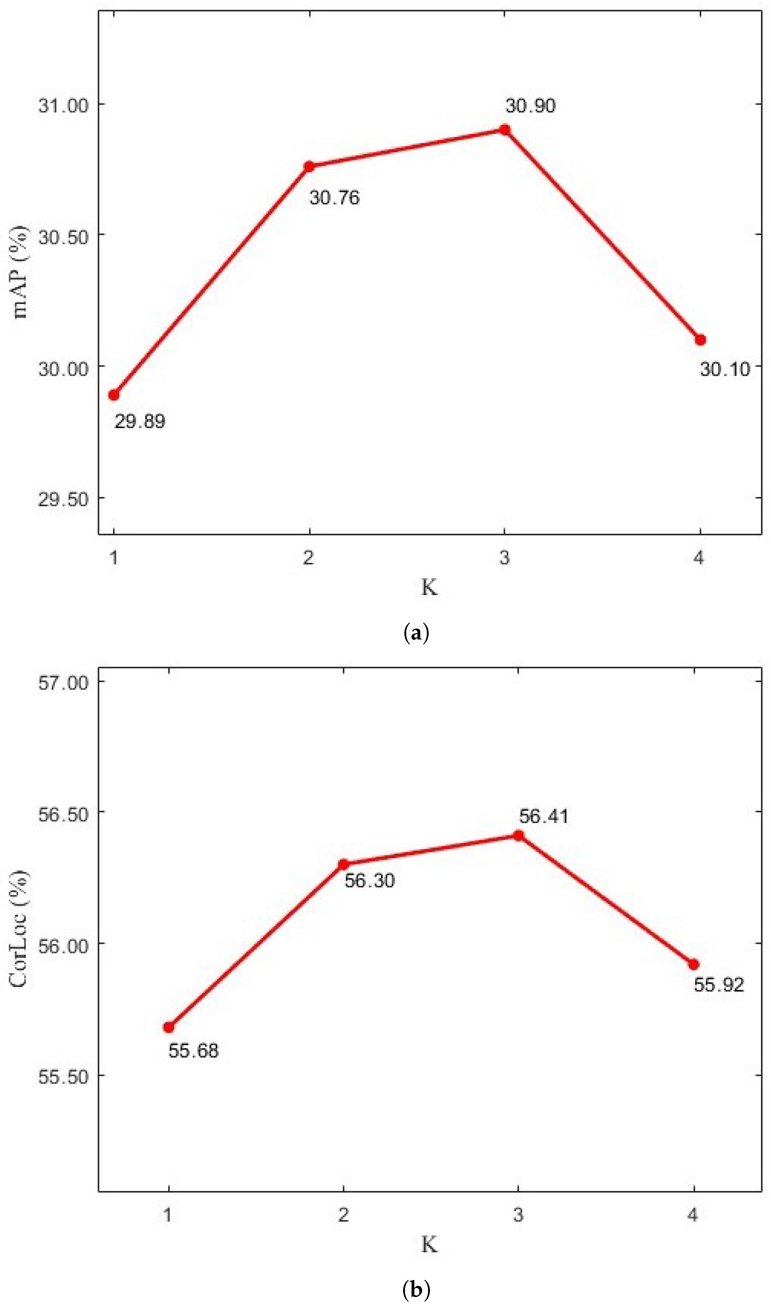
K (the number of PFSOD Heads) was analyzed on the DIOR dataset, as shown in Figure 4; both the mAP and CorLoc achieved the highest scores when K was set to 3.
5.3. Ablation Study
The ablation studies were conducted on the more challenging DIOR dataset to verify the effectiveness of the SSIM and SPGTM modules. As mentioned before, the “OICR+BBR” was adopted as the baseline [10,32,50]. As shown in Table 1, the mAP (CorLoc) increased by 5.63% and 6.71% (5.82% and 7.10%) when the SSIM and SPGTM modules were separately added to the baseline, respectively, which validates the effectiveness of the two modules. The mAP (CorLoc) improved by 10.80% (13.62%) when both the SSIM and SPGTM modules were added to the baseline, which proves the validity of the combination of the two modules.
5.4. Comparisons with Other Methods
5.4.1. Comparisons in Terms of mAP
As shown in Table 2 and Table 3, the mAP of our method achieved 73.4% (30.9%) on the NWPU VHR-10.v2 (DIOR) dataset, which outperformed the WSDDN [30], OICR [31], PCL [37], MELM [69], MIST [32], DCL [70], PCIR [41], MIG [34], TCA [42], SAE [64], SPG [38], MHQ-PSL [9], SGPLM-IR [11], RINet [62], and AE-IS [13]. Obviously, our method gave the optimal performance in terms of the mAP on the two RSI datasets.
5.4.2. Comparisons in Terms of CorLoc
As shown in Table 4 and Table 5, the CorLoc of our method achieved 78.7% (56.4%) on the NWPU VHR-10.v2 (DIOR) dataset, which outperformed the WSDDN, OICR, PCL, MELM, MIST, PCIR, MIG, TCA, SAE, SPG, MHQ-PSL, SGPLM-IR, RINet, and AE-IS. Obviously, our method also gave the best performance in terms of CorLoc on the two RSI datasets.
In conclusion, the overall capability of our method was superior to the other WSOD methods.
In addition, as shown in Table 2 and Table 3, our model was compared with two FSOD methods, i.e., fast R-CNN [1] and faster R-CNN [2]; the comparison results showed that our model significantly narrowed the gap between the WSOD and FSOD methods. Note that the capability of our method was almost comparable with the 2 FSOD methods on the NWPU VHR-10.v2 dataset.
5.5. Subjective Evaluation
6. Conclusions
A novel SPFS model that includes the SSIM and SPGTM modules is proposed in this article. First of all, the SIs mined by the CS tend to concentrate on the most significant parts of the target; moreover, they are unreliable because the reliability of the CS is not sufficient for RSIs with complex backgrounds. The SSIM module was proposed to address the aforementioned problem, which mines the SIs by using the OQS, which can represent the comprehensive characteristic of the category and the completeness of the target. Secondly, the localization capability of current methods is restricted because it solely depends on the proposals generated by the SS or EB, which is an early method and does not use the deep learning techniques. The SPGTM module was proposed to address the aforementioned problem, which can make full use of the advantages of SAM to obtain good-quality PGT instances, for which the localization was more accurate than the traditional proposals, and the PFSOD heads were trained by the PGT instances in a fully supervised manner. The ablation experiments verified the validity of the SSIM, SPGTM, and their integration. The quantitative comparisons with 15 WSOD methods demonstrated the excellent capability of our method.
Author Contributions
Conceptualization, X.Q.; formal analysis, X.Q.; funding acquisition, X.Q.; methodology, X.Q. and C.L.; project administration, W.W.; resources, W.W.; software, C.L.; supervision, W.W.; validation, W.W. and Z.C.; writing—original draft, C.L.; writing—review and editing, X.Q. and Z.C. All authors have read and agreed to the published version of the manuscript.
Funding
This work is supported by the National Natural Science Foundation of China (Grant No. 62076223), the Key Research Project of Henan Province Universities (Grant No. 24ZX005), and the Key Science and Technology Program of Henan Province (Grant No. 232102211018).
Data Availability Statement
The NWPU VHR-10.v2 and DIOR datasets are available at the following URLs: https://drive.google.com/file/d/15xd4TASVAC2irRf02GA4LqYFbH7QITR-/view (accessed on 15 March 2023) and https://drive.google.com/drive/folders/1UdlgHk49iu6WpcJ5467iT-UqNPpx__CC (accessed on 15 March 2023), respectively.
Conflicts of Interest
The authors declare no conflicts of interest.
Abbreviations
The following abbreviations are used in this manuscript:
| WSOD | weakly supervised object detection |
| RSI | remote sensing image |
| SI | seed instance |
| PGT | pseudo-ground truth |
| SSIM | SAM-induced seed instance mining |
| SPGTM | SAM-based pseudo-ground truth mining |
| OCS | object completeness score |
| OQS | object quality score |
| PFSOD | pseudo-fully supervised object detection |
References
- Girshick, R. Fast r-cnn. In Proceedings of the IEEE International Conference on Computer Vision, Washington, DC, USA, 7–13 December 2015; pp. 1440–1448. [Google Scholar]
- Ren, S.; He, K.; Girshick, R.; Sun, J. Faster R-CNN: Towards real-time object detection with region proposal networks. IEEE Trans. Pattern Anal. Mach. Intell. 2016, 39, 1137–1149. [Google Scholar] [CrossRef]
- Qian, X.; Wu, B.; Cheng, G.; Yao, X.; Wang, W.; Han, J. Building a Bridge of Bounding Box Regression Between Oriented and Horizontal Object Detection in Remote Sensing Images. IEEE Trans. Geosci. Remote Sens. 2023, 61, 1–9. [Google Scholar] [CrossRef]
- Li, L.; Yao, X.; Wang, X.; Hong, D.; Cheng, G.; Han, J. Robust Few-Shot Aerial Image Object Detection via Unbiased Proposals Filtration. IEEE Trans. Geosci. Remote Sens. 2023, 61, 1–11. [Google Scholar] [CrossRef]
- Cheng, G.; Li, Q.; Wang, G.; Xie, X.; Min, L.; Han, J. SFRNet: Fine-Grained Oriented Object Recognition via Separate Feature Refinement. IEEE Trans. Geosci. Remote Sens. 2023, 61, 1–10. [Google Scholar] [CrossRef]
- Xie, X.; Lang, C.; Miao, S.; Cheng, G.; Li, K.; Han, J. Mutual-Assistance Learning for Object Detection. IEEE Trans. Pattern Anal. Mach. Intell. 2023, 45, 15171–15184. [Google Scholar] [CrossRef]
- Xie, X.; Cheng, G.; Li, Q.; Miao, S.; Li, K.; Han, J. Fewer is more: Efficient object detection in large aerial images. Sci. China Inf. Sci. 2024, 67, 112106. [Google Scholar] [CrossRef]
- Liang, Y.; Feng, J.; Zhang, X.; Zhang, J.; Jiao, L. MidNet: An anchor-and-angle-free detector for oriented ship detection in aerial images. IEEE Trans. Geosci. Remote Sens. 2023, 61, 1–13. [Google Scholar] [CrossRef]
- Qian, X.; Huo, Y.; Cheng, G.; Gao, C.; Yao, X.; Wang, W. Mining High-Quality Pseudoinstance Soft Labels for Weakly Supervised Object Detection in Remote Sensing Images. IEEE Trans. Geosci. Remote Sens. 2023, 61, 1–15. [Google Scholar] [CrossRef]
- Qian, X.; Huo, Y.; Cheng, G.; Yao, X.; Li, K.; Ren, H.; Wang, W. Incorporating the completeness and difficulty of proposals into weakly supervised object detection in remote sensing images. IEEE J. Sel. Top. Appl. Earth Obs. Remote Sens. 2022, 15, 1902–1911. [Google Scholar] [CrossRef]
- Qian, X.; Li, C.; Wang, W.; Yao, X.; Cheng, G. Semantic segmentation guided pseudo label mining and instance re-detection for weakly supervised object detection in remote sensing images. Int. J. Appl. Earth Obs. Geoinf. 2023, 119, 103301. [Google Scholar] [CrossRef]
- Qian, X.; Wang, C.; Li, C.; Li, Z.; Zeng, L.; Wang, W.; Wu, Q. Multiscale Image Splitting Based Feature Enhancement and Instance Difficulty Aware Training for Weakly Supervised Object Detection in Remote Sensing Images. IEEE J. Sel. Top. Appl. Earth Obs. Remote Sens. 2023, 16, 7497–7506. [Google Scholar] [CrossRef]
- Xie, X.; Cheng, G.; Feng, X.; Yao, X.; Qian, X.; Han, J. Attention Erasing and Instance Sampling for Weakly Supervised Object Detection. IEEE Trans. Geosci. Remote Sens. 2024, 62, 1–10. [Google Scholar] [CrossRef]
- Wu, Z.; Wen, J.; Xu, Y.; Yang, J.; Li, X.; Zhang, D. Enhanced spatial feature learning for weakly supervised object detection. IEEE Trans. Neural Netw. Learn. Syst. 2022, 35, 961–972. [Google Scholar] [CrossRef]
- Wu, Z.; Wen, J.; Xu, Y.; Yang, J.; Zhang, D. Multiple instance detection networks with adaptive instance refinement. IEEE Trans. Multimed. 2021, 25, 267–279. [Google Scholar] [CrossRef]
- Zhang, D.; Li, H.; Zeng, W.; Fang, C.; Cheng, L.; Cheng, M.M.; Han, J. Weakly Supervised Semantic Segmentation via Alternate Self-Dual Teaching. IEEE Trans. Image Process. 2023, 72, 1. [Google Scholar] [CrossRef]
- Zhang, D.; Guo, G.; Zeng, W.; Li, L.; Han, J. Generalized weakly supervised object localization. IEEE Trans. Neural Netw. Learn. Syst. 2022, 35, 5395–5406. [Google Scholar] [CrossRef]
- Tong, W.; Chen, W.; Han, W.; Li, X.; Wang, L. Channel-attention-based DenseNet network for remote sensing image scene classification. IEEE J. Sel. Top. Appl. Earth Obs. Remote Sens. 2020, 60, 4121–4132. [Google Scholar] [CrossRef]
- Chen, W.; Ouyang, S.; Tong, W.; Li, X.; Zheng, X.; Wang, L. GCSANet: A global context spatial attention deep learning network for remote sensing scene classification. IEEE J. Sel. Top. Appl. Earth Obs. Remote Sens. 2022, 60, 1150–1162. [Google Scholar] [CrossRef]
- Tekumalla, R.; Banda, J.M. TweetDIS: A large twitter dataset for natural disasters built using weak supervision. In Proceedings of the 2022 IEEE International Conference on Big Data (Big Data), Osaka, Japan, 17–20 December 2022; Volume 60, pp. 4816–4823. [Google Scholar] [CrossRef]
- Presa-Reyes, M.; Tao, Y.; Chen, S.C.; Shyu, M.L. Deep learning with weak supervision for disaster scene description in low-altitude imagery. IEEE Trans. Geosci. Remote Sens. 2021, 60, 1–10. [Google Scholar] [CrossRef]
- Tang, W.; Deng, C.; Han, Y.; Huang, Y.; Zhao, B. SRARNet: A unified framework for joint superresolution and aircraft recognition. IEEE J. Sel. Top. Appl. Earth Obs. Remote Sens. 2020, 14, 327–336. [Google Scholar] [CrossRef]
- He, Q.; Sun, X.; Yan, Z.; Li, B.; Fu, K. Multi-object tracking in satellite videos with graph-based multitask modeling. IEEE Trans. Geosci. Remote Sens. 2022, 60, 1–13. [Google Scholar] [CrossRef]
- Lin, S.; Zhang, M.; Cheng, X.; Shi, L.; Gamba, P.; Wang, H. Dynamic Low-Rank and Sparse Priors Constrained Deep Autoencoders for Hyperspectral Anomaly Detection. IEEE Trans. Instrum. Meas. 2023, 73, 2500518. [Google Scholar] [CrossRef]
- Lin, S.; Zhang, M.; Cheng, X.; Zhou, K.; Zhao, S.; Wang, H. Hyperspectral Anomaly Detection via Sparse Representation and Collaborative Representation. IEEE J. Sel. Top. Appl. Earth Obs. Remote Sens. 2023, 16, 946–961. [Google Scholar] [CrossRef]
- Lin, S.; Zhang, M.; Cheng, X.; Zhou, K.; Zhao, S.; Wang, H. Dual Collaborative Constraints Regularized Low-Rank and Sparse Representation via Robust Dictionaries Construction for Hyperspectral Anomaly Detection. IEEE J. Sel. Top. Appl. Earth Obs. Remote Sens. 2023, 16, 2009–2024. [Google Scholar] [CrossRef]
- Cheng, X.; Zhang, M.; Lin, S.; Li, Y.; Wang, H. Deep Self-Representation Learning Framework for Hyperspectral Anomaly Detection. IEEE Trans. Instrum. Meas. 2023, 73, 5002016. [Google Scholar] [CrossRef]
- Cheng, X.; Zhang, M.; Lin, S.; Zhou, K.; Zhao, S.; Wang, H. Two-Stream Isolation Forest Based on Deep Features for Hyperspectral Anomaly Detection. IEEE Geosci. Remote Sens. Lett. 2023, 20, 1–5. [Google Scholar] [CrossRef]
- Huo, Y.; Qian, X.; Li, C.; Wang, W. Multiple Instance Complementary Detection and Difficulty Evaluation for Weakly Supervised Object Detection in Remote Sensing Images. IEEE Geosci. Remote Sens. Lett. 2023, 20, 1–5. [Google Scholar] [CrossRef]
- Bilen, H.; Vedaldi, A. Weakly supervised deep detection networks. In Proceedings of the IEEE Conference on Computer Vision and Pattern Recognition (CVPR), Las Vegas, NV, USA, 27–30 June 2016; pp. 2846–2854. [Google Scholar]
- Tang, P.; Wang, X.; Bai, X.; Liu, W. Multiple instance detection network with online instance classifier refinement. In Proceedings of the IEEE Conference on Computer Vision and Pattern Recognition (CVPR), Honolulu, HI, USA, 21–26 July 2017; pp. 2843–2851. [Google Scholar]
- Ren, Z.; Yu, Z.; Yang, X.; Liu, M.Y.; Lee, Y.J.; Schwing, A.G.; Kautz, J. Instance-aware, context-focused, and memory-efficient weakly supervised object detection. In Proceedings of the IEEE/CVF Conference on Computer Vision and Pattern Recognition, Seattle, WA, USA, 13–19 June 2020; pp. 10598–10607. [Google Scholar]
- Yin, Y.; Deng, J.; Zhou, W.; Li, L.; Li, H. Fi-wsod: Foreground information guided weakly supervised object detection. IEEE Trans. Multimed. 2022, 25, 1890–1902. [Google Scholar] [CrossRef]
- Wang, B.; Zhao, Y.; Li, X. Multiple instance graph learning for weakly supervised remote sensing object detection. IEEE Trans. Geosci. Remote Sens. 2021, 60, 1–12. [Google Scholar] [CrossRef]
- Uijlings, J.R.; Van De Sande, K.E.; Gevers, T.; Smeulders, A.W. Selective search for object recognition. Int. J. Comput. Vis. 2013, 104, 154–171. [Google Scholar] [CrossRef]
- Wei, Y.; Shen, Z.; Cheng, B.; Shi, H.; Xiong, J.; Feng, J.; Huang, T. Ts2c: Tight box mining with surrounding segmentation context for weakly supervised object detection. In Proceedings of the European Conference on Computer Vision (ECCV), Munich, Germany, 8–14 September 2018; pp. 434–450. [Google Scholar] [CrossRef]
- Tang, P.; Wang, X.; Bai, S.; Shen, W.; Bai, X.; Liu, W.; Yuille, A. PCL: Proposal Cluster Learning for Weakly Supervised Object Detection. IEEE Trans. Pattern Anal. Mach. Intell. 2020, 42, 176–191. [Google Scholar] [CrossRef]
- Cheng, G.; Xie, X.; Chen, W.; Feng, X.; Yao, X.; Han, J. Self-guided proposal generation for weakly supervised object detection. IEEE Trans. Geosci. Remote Sens. 2022, 60, 1–11. [Google Scholar] [CrossRef]
- Xia, R.; Li, G.; Huang, Z.; Meng, H.; Pang, Y. CBASH: Combined backbone and advanced selection heads with object semantic proposals for weakly supervised object detection. IEEE Trans. Circuits Syst. Video Technol. 2022, 32, 6502–6514. [Google Scholar] [CrossRef]
- Wu, Z.; Liu, C.; Wen, J.; Xu, Y.; Yang, J.; Li, X. Selecting high-quality proposals for weakly supervised object detection with bottom-up aggregated attention and phase-aware loss. IEEE Trans. Image Process. 2022, 32, 682–693. [Google Scholar] [CrossRef]
- Feng, X.; Han, J.; Yao, X.; Cheng, G. Progressive contextual instance refinement for weakly supervised object detection in remote sensing images. IEEE Trans. Geosci. Remote Sens. 2020, 58, 8002–8012. [Google Scholar] [CrossRef]
- Feng, X.; Han, J.; Yao, X.; Cheng, G. TCANet: Triple context-aware network for weakly supervised object detection in remote sensing images. IEEE Trans. Geosci. Remote Sens. 2021, 59, 6946–6955. [Google Scholar] [CrossRef]
- Zitnick, C.L.; Dollár, P. Edge boxes: Locating object proposals from edges. In Proceedings of the Computer Vision–ECCV 2014: 13th European Conference, Zurich, Switzerland, 6–12 September 2014; Proceedings, Part V 13, 2014. pp. 391–405. [Google Scholar] [CrossRef]
- Lin, C.; Wang, S.; Xu, D.; Lu, Y.; Zhang, W. Object instance mining for weakly supervised object detection. Proc. AAAI Conf. Artif. Intell. 2020, 34, 11482–11489. [Google Scholar] [CrossRef]
- Feng, J.; Liang, Y.; Zhang, X.; Zhang, J.; Jiao, L. SDANet: Semantic-embedded density adaptive network for moving vehicle detection in satellite videos. IEEE Trans. Image Process. 2023, 32, 1788–1801. [Google Scholar] [CrossRef]
- Feng, J.; Bai, G.; Li, D.; Zhang, X.; Shang, R.; Jiao, L. MR-selection: A meta-reinforcement learning approach for zero-shot hyperspectral band selection. IEEE Trans. Geosci. Remote Sens. 2022, 61, 1–20. [Google Scholar] [CrossRef]
- Qian, X.; Zeng, Y.; Wang, W.; Zhang, Q. Co-Saliency Detection Guided by Group Weakly Supervised Learning. IEEE Trans. Multimed. 2023, 25, 1810–1818. [Google Scholar] [CrossRef]
- Feng, J.; Gao, Z.; Shang, R.; Zhang, X.; Jiao, L. Multi-complementary generative adversarial networks with contrastive learning for hyperspectral image classification. IEEE Trans. Geosci. Remote Sens. 2023, 61, 1–18. [Google Scholar] [CrossRef]
- Qian, X.; Zhang, N.; Wang, W. Smooth giou loss for oriented object detection in remote sensing images. Remote Sens. 2023, 15, 1259. [Google Scholar] [CrossRef]
- Seo, J.; Bae, W.; Sutherland, D.J.; Noh, J.; Kim, D. Object Discovery via Contrastive Learning for Weakly Supervised Object Detection. In Proceedings of the Computer Vision—ECCV 2022; Springer Nature: Cham, Switzerland, 2022; pp. 312–329. [Google Scholar]
- Kirillov, A.; Mintun, E.; Ravi, N.; Mao, H.; Rolland, C.; Gustafson, L.; Xiao, T.; Whitehead, S.; Berg, A.C.; Lo, W.Y.; et al. Segment anything. arXiv 2023, arXiv:2304.02643. [Google Scholar] [CrossRef]
- Zhou, B.; Khosla, A.; Lapedriza, A.; Oliva, A.; Torralba, A. Learning deep features for discriminative localization. In Proceedings of the IEEE Conference on Computer Vision and Pattern Recognition, New York, NY, USA, 15–17 June 2016; pp. 2921–2929. [Google Scholar] [CrossRef]
- Selvaraju, R.R.; Cogswell, M.; Das, A.; Vedantam, R.; Parikh, D.; Batra, D. Grad-cam: Visual explanations from deep networks via gradient-based localization. In Proceedings of the IEEE International Conference on Computer Vision, Venice, Italy, 22–29 October 2017; pp. 618–626. [Google Scholar] [CrossRef]
- He, K.; Gkioxari, G.; Dollár, P.; Girshick, R. Mask r-cnn. In Proceedings of the IEEE International Conference on Computer Vision, Venice, Italy, 22–29 October 2017; pp. 2961–2969. [Google Scholar] [CrossRef]
- Cheng, G.; Zhou, P.; Han, J. Learning Rotation-Invariant Convolutional Neural Networks for Object Detection in VHR Optical Remote Sensing Images. IEEE Trans. Geosci. Remote Sens. 2016, 54, 7405–7415. [Google Scholar] [CrossRef]
- Li, K.; Cheng, G.; Bu, S.; You, X. Rotation-Insensitive and Context-Augmented Object Detection in Remote Sensing Images. IEEE Trans. Geosci. Remote Sens. 2018, 56, 2337–2348. [Google Scholar] [CrossRef]
- Li, K.; Wan, G.; Cheng, G.; Meng, L.; Han, J. Object detection in optical remote sensing images: A survey and a new benchmark. ISPRS J. Photogramm. Remote Sens. 2020, 159, 296–307. [Google Scholar] [CrossRef]
- Deselaers, T.; Alexe, B.; Ferrari, V. Weakly supervised localization and learning with generic knowledge. Int. J. Comput. Vis. 2012, 100, 275–293. [Google Scholar] [CrossRef]
- Simonyan, K.; Zisserman, A. Very deep convolutional networks for large-scale image recognition. arXiv 2014, arXiv:1409.1556. [Google Scholar]
- Krizhevsky, A.; Sutskever, I.; Hinton, G.E. ImageNet Classification with Deep Convolutional Neural Networks. Adv. Neural Inf. Process. Syst. 2012, 25, 1097–1105. [Google Scholar] [CrossRef]
- Hosang, J.; Benenson, R.; Schiele, B. Learning non-maximum suppression. In Proceedings of the IEEE Conference on Computer Vision and Pattern Recognition (CVPR), Honolulu, HI, USA, 21–26 July 2017; pp. 4507–4515. [Google Scholar]
- Feng, X.; Yao, X.; Cheng, G.; Han, J. Weakly Supervised Rotation-Invariant Aerial Object Detection Network. In Proceedings of the 2022 IEEE/CVF Conference on Computer Vision and Pattern Recognition (CVPR), New Orleans, LA, USA, 18–24 June 2022; pp. 14126–14135. [Google Scholar] [CrossRef]
- Chen, Z.; Fu, Z.; Jiang, R.; Chen, Y.; Hua, X.S. Slv: Spatial likelihood voting for weakly supervised object detection. In Proceedings of the IEEE/CVF Conference on Computer Vision and Pattern Recognition, Seattle, WA, USA, 13–19 June 2020; pp. 12995–13004. [Google Scholar] [CrossRef]
- Feng, X.; Yao, X.; Cheng, G.; Han, J.; Han, J. SAENet: Self-Supervised Adversarial and Equivariant Network for Weakly Supervised Object Detection in Remote Sensing Images. IEEE Trans. Geosci. Remote Sens. 2022, 60, 1–11. [Google Scholar] [CrossRef]
- Yang, K.; Zhang, P.; Qiao, P.; Wang, Z.; Dai, H.; Shen, T.; Li, D.; Dou, Y. Rethinking Segmentation Guidance for Weakly Supervised Object Detection. In Proceedings of the 2020 IEEE/CVF Conference on Computer Vision and Pattern Recognition Workshops (CVPRW), Seattle, WA, USA, 14–19 June 2020; pp. 4069–4073. [Google Scholar] [CrossRef]
- Wang, G.; Zhang, X.; Peng, Z.; Jia, X.; Tang, X.; Jiao, L. MOL: Towards accurate weakly supervised remote sensing object detection via Multi-view nOisy Learning. ISPRS J. Photogramm. Remote Sens. 2023, 196, 457–470. [Google Scholar] [CrossRef]
- Chen, M.; Tian, Y.; Li, Z.; Li, E.; Liang, Z. Online Progressive Instance-Balanced Sampling for Weakly Supervised Vibration Damper Detection. IEEE Trans. Instrum. Meas. 2023, 72, 1–14. [Google Scholar] [CrossRef]
- Wang, G.; Zhang, X.; Peng, Z.; Tang, X.; Zhou, H.; Jiao, L. Absolute wrong makes better: Boosting weakly supervised object detection via negative deterministic information. arXiv 2022, arXiv:2204.10068. [Google Scholar] [CrossRef]
- Wan, F.; Wei, P.; Jiao, J.; Han, Z.; Ye, Q. Min-entropy latent model for weakly supervised object detection. In Proceedings of the IEEE Conference Computer Vision and Pattern Recognition, Salt Lake City, UT, USA, 18–22 June 2018; pp. 1297–1306. [Google Scholar]
- Yao, X.; Feng, X.; Han, J.; Cheng, G.; Guo, L. Automatic weakly supervised object detection from high spatial resolution remote sensing images via dynamic curriculum learning. IEEE Trans. Geosci. Remote Sens. 2020, 59, 675–685. [Google Scholar] [CrossRef]
Figure 1.
The framework of the proposed method. The WSDDN, SSIM, and SPGTM modules and PFSOD heads are introduced in Section 3.1, Section 4.2, Section 4.3, and Section 4.4, respectively.
Figure 1.
The framework of the proposed method. The WSDDN, SSIM, and SPGTM modules and PFSOD heads are introduced in Section 3.1, Section 4.2, Section 4.3, and Section 4.4, respectively.

Figure 2.
The number of object instances for each category in the two datasets.

Figure 3.
The values of (a) mAP and (b) CorLoc with respect to different on the DIOR dataset.

Figure 4.
The values of (a) mAP and (b) CorLoc with respect to different K on the DIOR dataset.

Figure 5.
Visualization of some results of the SPFS model on the NWPU VHR-10.v2 dataset.

Figure 6.
Visualization of some results of the SPFS model on the DIOR dataset.


Table 1.
Ablation studies of SSIM and SPGTM on the DIOR dataset.
| Baseline | SSIM | SPGTM | mAP | CorLoc |
|---|---|---|---|---|
| ✓ | 20.10 | 42.79 | ||
| ✓ | ✓ | 25.73 | 48.61 | |
| ✓ | ✓ | 26.81 | 49.89 | |
| ✓ | ✓ | ✓ | 30.90 | 56.41 |
Table 2.
The comparisons of average precision (%) with other methods on the NWPU VHR-10.v2 dataset. The bold font denotes the best result. The same below.
Table 2.
The comparisons of average precision (%) with other methods on the NWPU VHR-10.v2 dataset. The bold font denotes the best result. The same below.
| Method | Airplane | Ship | Storage Tank | Baseball Diamond | Tennis Court | Basketball Court | Ground Track Field | Harbor | Bridge | Vehicle | mAP |
|---|---|---|---|---|---|---|---|---|---|---|---|
| Fast R-CNN [1] | 90.91 | 90.60 | 89.29 | 47.32 | 100.00 | 85.85 | 84.86 | 88.22 | 80.29 | 69.84 | 82.72 |
| Faster R-CNN [2] | 90.90 | 86.30 | 90.53 | 98.24 | 89.72 | 69.64 | 100.00 | 80.11 | 61.49 | 78.14 | 84.51 |
| WSDDN [30] | 30.08 | 41.72 | 35.98 | 88.90 | 12.86 | 23.85 | 99.43 | 13.94 | 1.92 | 3.60 | 35.12 |
| OICR [31] | 13.66 | 67.35 | 57.16 | 55.16 | 13.64 | 39.66 | 92.80 | 0.23 | 1.84 | 3.73 | 34.52 |
| PCL [37] | 26.00 | 63.76 | 2.50 | 89.80 | 64.45 | 76.07 | 77.94 | 0.00 | 1.30 | 15.67 | 39.41 |
| MELM [69] | 80.86 | 69.30 | 10.48 | 90.17 | 12.84 | 20.14 | 99.17 | 17.10 | 14.17 | 8.68 | 42.29 |
| MIST [32] | 69.69 | 49.16 | 48.55 | 80.91 | 27.08 | 79.85 | 91.34 | 46.99 | 8.29 | 13.36 | 51.52 |
| DCL [70] | 72.70 | 74.25 | 37.05 | 82.64 | 36.88 | 42.27 | 83.95 | 39.57 | 16.82 | 35.00 | 52.11 |
| PCIR [41] | 90.78 | 78.81 | 36.40 | 90.80 | 22.64 | 52.16 | 88.51 | 42.36 | 11.74 | 35.49 | 54.97 |
| MIG [34] | 88.69 | 71.61 | 75.17 | 94.19 | 37.45 | 47.68 | 100.00 | 27.27 | 8.33 | 9.06 | 55.95 |
| TCA [42] | 89.43 | 78.18 | 78.42 | 90.80 | 35.27 | 50.36 | 90.91 | 42.44 | 4.11 | 28.30 | 58.82 |
| SAE [64] | 82.91 | 74.47 | 50.20 | 96.74 | 55.66 | 72.94 | 100.00 | 36.46 | 6.33 | 31.89 | 60.76 |
| SPG [38] | 90.42 | 81.00 | 59.53 | 92.31 | 35.64 | 51.44 | 99.92 | 58.71 | 16.99 | 42.99 | 62.89 |
| MHQ-PSL [9] | 87.60 | 81.00 | 57.30 | 94.00 | 36.40 | 80.40 | 100.00 | 56.90 | 9.80 | 35.60 | 63.80 |
| SGPLM-IR [11] | 90.70 | 79.90 | 69.30 | 97.50 | 41.60 | 77.50 | 100.00 | 44.40 | 17.20 | 33.50 | 65.20 |
| RINet [62] | 90.30 | 86.30 | 79.60 | 90.70 | 58.20 | 80.40 | 100.00 | 57.70 | 18.90 | 41.60 | 70.40 |
| AE-IS [13] | 91.00 | 88.20 | 78.30 | 93.20 | 60.60 | 82.40 | 100.00 | 60.40 | 19.60 | 45.80 | 72.00 |
| SPFS (ours) | 91.23 | 83.32 | 73.64 | 90.56 | 73.10 | 85.28 | 100.00 | 63.59 | 10.24 | 63.52 | 73.45 |
Table 3.
The comparisons of average precision (%) with other methods on the DIOR dataset.
| Method | Airplane | Airport | Baseball Field | Basketball Court | Bridge | Chimney | Dam | Expressway Service Area | Expressway Toll Station | Golf Field | |
|---|---|---|---|---|---|---|---|---|---|---|---|
| Fast R-CNN [1] | 44.17 | 66.79 | 66.96 | 60.49 | 15.56 | 72.28 | 51.95 | 65.87 | 44.76 | 72.11 | |
| Faster R-CNN [2] | 50.28 | 62.60 | 66.04 | 80.88 | 28.80 | 68.17 | 47.26 | 58.51 | 48.06 | 60.44 | |
| WSDDN [30] | 9.06 | 39.68 | 37.81 | 20.16 | 0.25 | 12.28 | 0.57 | 0.65 | 11.88 | 4.90 | |
| OICR [31] | 8.70 | 28.26 | 44.05 | 18.22 | 1.30 | 20.15 | 0.09 | 0.65 | 29.89 | 13.80 | |
| PCL [37] | 21.52 | 35.19 | 59.80 | 23.49 | 2.95 | 43.71 | 0.12 | 0.90 | 1.49 | 2.88 | |
| MELM [69] | 28.14 | 3.23 | 62.51 | 28.72 | 0.06 | 62.51 | 0.21 | 28.39 | 13.09 | 15.15 | |
| MIST [32] | 32.01 | 39.87 | 62.71 | 28.97 | 7.46 | 12.87 | 0.31 | 5.14 | 17.38 | 51.02 | |
| DCL [70] | 20.89 | 22.70 | 54.21 | 11.50 | 6.03 | 61.01 | 0.09 | 1.07 | 31.01 | 30.87 | |
| PCIR [41] | 30.37 | 36.06 | 54.22 | 26.60 | 9.09 | 58.59 | 0.22 | 9.65 | 36.18 | 32.59 | |
| MIG [34] | 22.20 | 52.57 | 62.76 | 25.78 | 8.47 | 67.42 | 0.66 | 8.85 | 28.71 | 57.28 | |
| TCA [42] | 25.13 | 30.84 | 62.92 | 40.00 | 4.13 | 67.78 | 8.07 | 23.80 | 29.89 | 22.34 | |
| SAE [64] | 20.57 | 62.41 | 62.65 | 23.54 | 7.59 | 64.62 | 0.22 | 34.52 | 30.62 | 55.38 | |
| SPG [38] | 31.32 | 36.66 | 62.79 | 29.10 | 6.08 | 62.66 | 0.31 | 15.00 | 30.10 | 35.00 | |
| MHQ-PSL [9] | 29.10 | 49.80 | 70.90 | 41.40 | 7.20 | 45.50 | 0.20 | 35.40 | 36.80 | 60.80 | |
| SGPLM-IR [11] | 39.10 | 64.60 | 64.40 | 26.90 | 6.30 | 62.30 | 0.90 | 12.20 | 26.30 | 55.30 | |
| RINet [62] | 26.20 | 57.40 | 62.70 | 25.10 | 9.90 | 69.20 | 1.40 | 13.30 | 36.20 | 51.40 | |
| AE-IS [13] | 31.80 | 50.90 | 63.20 | 29.40 | 8.90 | 68.70 | 1.30 | 15.10 | 35.50 | 51.60 | |
| SPFS (ours) | 35.94 | 62.89 | 66.08 | 30.53 | 9.71 | 69.77 | 1.93 | 12.88 | 34.90 | 50.49 | |
| Method | Ground Track Field | Harbor | Overpass | Ship | Stadium | Storage Tank | Tennis Court | Train Station | Vehicle | Windmill | mAP |
| Fast R-CNN [1] | 62.93 | 46.18 | 38.03 | 32.13 | 70.98 | 35.04 | 58.27 | 37.91 | 19.20 | 38.10 | 49.98 |
| Faster R-CNN [2] | 67.00 | 43.86 | 46.87 | 58.48 | 52.37 | 42.35 | 79.52 | 48.02 | 34.77 | 65.44 | 55.49 |
| WSDDN [30] | 42.53 | 4.66 | 1.06 | 0.70 | 63.03 | 3.95 | 6.06 | 0.51 | 4.55 | 1.14 | 13.27 |
| OICR [31] | 57.39 | 10.66 | 11.06 | 9.09 | 59.29 | 7.10 | 0.68 | 0.14 | 9.09 | 0.41 | 16.50 |
| PCL [37] | 56.36 | 16.76 | 11.05 | 9.09 | 57.62 | 9.09 | 2.47 | 0.12 | 4.55 | 4.5 | 18.19 |
| MELM [69] | 41.05 | 26.12 | 0.43 | 9.09 | 8.28 | 15.02 | 20.57 | 9.81 | 0.04 | 0.53 | 18.65 |
| MIST [32] | 49.48 | 5.36 | 12.24 | 29.43 | 35.53 | 25.36 | 0.81 | 4.59 | 22.22 | 0.80 | 22.18 |
| DCL [70] | 56.45 | 5.05 | 2.65 | 9.09 | 63.65 | 9.09 | 10.36 | 0.02 | 7.27 | 0.79 | 20.19 |
| PCIR [41] | 58.51 | 8.60 | 21.63 | 12.09 | 64.28 | 9.09 | 13.62 | 0.30 | 9.09 | 7.52 | 24.92 |
| MIG [34] | 47.73 | 23.77 | 0.77 | 6.42 | 54.13 | 13.15 | 4.12 | 14.76 | 0.23 | 2.43 | 25.11 |
| TCA [42] | 53.85 | 24.84 | 11.06 | 9.09 | 46.40 | 13.74 | 30.98 | 1.47 | 9.09 | 1.00 | 25.82 |
| SAE [64] | 52.70 | 17.57 | 6.85 | 9.09 | 51.59 | 15.43 | 1.69 | 14.44 | 1.41 | 9.16 | 27.10 |
| SPG [38] | 48.02 | 27.11 | 12.00 | 10.02 | 60.04 | 15.10 | 21.00 | 9.92 | 3.15 | 0.06 | 25.77 |
| MHQ-PSL [9] | 48.50 | 14.00 | 25.10 | 18.50 | 48.90 | 11.70 | 11.90 | 3.50 | 11.30 | 1.70 | 28.60 |
| SGPLM-IR [11] | 60.60 | 9.40 | 23.10 | 13.40 | 57.40 | 17.70 | 1.50 | 14.00 | 11.50 | 3.50 | 28.50 |
| RINet [62] | 53.90 | 28.60 | 4.80 | 9.10 | 52.70 | 15.80 | 20.60 | 12.90 | 9.10 | 4.70 | 28.30 |
| AE-IS [13] | 52.30 | 28.80 | 13.30 | 11.20 | 56.90 | 16.30 | 22.40 | 14.00 | 8.00 | 2.60 | 29.10 |
| SPFS (ours) | 56.92 | 25.29 | 26.30 | 15.18 | 52.29 | 12.62 | 25.81 | 13.88 | 11.61 | 3.10 | 30.90 |
Table 4.
The comparisons of correct localization (%) with other methods on the NWPU VHR-10.v2 dataset.
Table 4.
The comparisons of correct localization (%) with other methods on the NWPU VHR-10.v2 dataset.
| Method | Airplane | Ship | Storage Tank | Baseball Diamond | Tennis Court | Basketball Court | Ground Track Field | Harbor | Bridge | Vehicle | mAP |
|---|---|---|---|---|---|---|---|---|---|---|---|
| WSDDN [30] | 22.32 | 36.81 | 39.95 | 92.48 | 17.96 | 24.24 | 99.26 | 14.83 | 1.69 | 2.89 | 35.24 |
| OICR [31] | 29.41 | 83.33 | 20.51 | 81.76 | 40.85 | 32.08 | 86.60 | 7.41 | 3.70 | 14.44 | 40.01 |
| PCL [37] | 11.76 | 50.00 | 12.82 | 98.65 | 84.51 | 77.36 | 90.72 | 0.00 | 9.26 | 15.56 | 45.06 |
| MELM [69] | 85.96 | 77.42 | 21.43 | 98.33 | 10.71 | 43.48 | 95.00 | 40.00 | 11.76 | 14.63 | 49.87 |
| MIST [32] | 90.20 | 82.50 | 80.30 | 98.60 | 48.50 | 87.40 | 98.30 | 66.50 | 14.60 | 35.80 | 70.30 |
| PCIR [41] | 100.00 | 93.06 | 64.10 | 99.32 | 64.79 | 79.25 | 89.69 | 62.96 | 13.26 | 52.22 | 71.87 |
| MIG [34] | 97.79 | 90.26 | 87.18 | 98.65 | 54.93 | 64.15 | 100.00 | 74.07 | 12.96 | 21.57 | 70.16 |
| TCA [42] | 96.91 | 91.78 | 95.13 | 88.65 | 66.90 | 62.83 | 95.98 | 54.18 | 19.63 | 55.50 | 72.76 |
| SAE [64] | 97.06 | 91.67 | 87.81 | 98.65 | 40.86 | 81.13 | 100.00 | 70.37 | 14.81 | 52.22 | 73.46 |
| SPG [38] | 98.06 | 92.67 | 70.08 | 99.65 | 51.86 | 80.12 | 96.20 | 72.44 | 12.99 | 60.02 | 73.41 |
| MHQ-PSL [9] | 94.40 | 86.60 | 68.50 | 97.80 | 69.80 | 87.50 | 100.00 | 68.60 | 16.00 | 56.60 | 74.60 |
| SGPLM-IR [11] | 98.20 | 93.80 | 89.30 | 99.10 | 50.20 | 88.90 | 100.00 | 71.00 | 12.30 | 51.20 | 75.40 |
| AE-IS [13] | 98.30 | 94.20 | 72.40 | 100.00 | 56.80 | 83.60 | 98.40 | 76.80 | 18.20 | 62.40 | 76.10 |
| SPFS (ours) | 95.49 | 90.32 | 81.53 | 90.18 | 70.10 | 89.94 | 100.0 | 78.90 | 19.38 | 70.81 | 78.67 |
Table 5.
The comparisons of correct localization (%) with other methods on the DIOR dataset.
| Method | Airplane | Airport | Baseball Field | Basketball Court | Bridge | Chimney | Dam | Expressway Service Area | Expressway Toll Station | Golf Field | |
|---|---|---|---|---|---|---|---|---|---|---|---|
| WSDDN [30] | 5.72 | 59.88 | 94.24 | 55.94 | 4.92 | 23.40 | 1.03 | 6.79 | 44.52 | 12.75 | |
| OICR [31] | 15.98 | 51.45 | 94.77 | 55.79 | 2.63 | 23.89 | 0.00 | 4.82 | 56.68 | 22.42 | |
| PCL [37] | 61.14 | 46.86 | 95.39 | 63.61 | 7.32 | 95.07 | 0.21 | 5.71 | 5.14 | 50.77 | |
| MELM [69] | 76.98 | 28.94 | 92.66 | 63.01 | 13.00 | 90.09 | 0.21 | 37.88 | 16.96 | 44.62 | |
| MIST [32] | 91.60 | 53.20 | 93.50 | 66.30 | 10.80 | 30.70 | 1.50 | 14.03 | 35.20 | 47.50 | |
| PCIR [41] | 93.10 | 45.60 | 95.50 | 68.30 | 3.60 | 92.10 | 0.20 | 5.40 | 58.40 | 47.50 | |
| MIG [34] | 76.98 | 46.86 | 95.39 | 63.61 | 23.00 | 95.07 | 0.21 | 16.96 | 57.88 | 50.77 | |
| TCA [42] | 81.58 | 51.33 | 96.17 | 73.45 | 5.03 | 94.69 | 15.89 | 32.79 | 45.95 | 48.56 | |
| SAE [64] | 91.20 | 69.37 | 95.48 | 67.52 | 18.88 | 97.78 | 0.21 | 70.54 | 54.32 | 51.43 | |
| SPG [38] | 80.48 | 32.04 | 98.68 | 65.00 | 15.20 | 96.08 | 22.52 | 16.99 | 46.08 | 50.96 | |
| MHQ-PSL [9] | 85.50 | 68.90 | 96.80 | 75.80 | 11.60 | 94.70 | 0.80 | 67.50 | 60.50 | 46.50 | |
| SGPLM-IR [11] | 92.20 | 58.30 | 97.80 | 74.20 | 16.20 | 95.20 | 0.30 | 51.30 | 56.20 | 52.30 | |
| RINet [62] | 92.70 | 80.90 | 92.70 | 69.50 | 8.60 | 90.10 | 0.20 | 71.30 | 62.00 | 65.50 | |
| AE-IS [13] | 91.40 | 78.60 | 96.10 | 68.80 | 16.00 | 92.30 | 22.80 | 68.90 | 60.60 | 62.70 | |
| SPFS (ours) | 90.82 | 80.13 | 98.59 | 65.50 | 19.45 | 90.38 | 2.35 | 70.61 | 62.24 | 66.51 | |
| Method | Ground Track Field | Harbor | Overpass | Ship | Stadium | Storage Tank | Tennis Court | Train Station | Vehicle | Windmill | mAP |
| WSDDN [30] | 89.90 | 5.45 | 10.00 | 22.96 | 98.54 | 79.61 | 15.06 | 3.45 | 11.56 | 3.22 | 32.44 |
| OICR [31] | 91.41 | 18.18 | 18.70 | 31.80 | 98.28 | 81.29 | 7.45 | 1.22 | 15.83 | 1.98 | 34.77 |
| PCL [37] | 89.39 | 42.12 | 19.78 | 37.94 | 97.93 | 80.65 | 13.77 | 0.20 | 10.50 | 6.94 | 41.52 |
| MELM [69] | 88.08 | 49.39 | 15.65 | 28.19 | 98.28 | 82.97 | 22.75 | 10.34 | 4.62 | 2.23 | 43.34 |
| MIST [32] | 87.10 | 38.60 | 23.40 | 50.70 | 80.50 | 89.20 | 22.40 | 11.50 | 22.20 | 2.40 | 43.60 |
| PCIR [41] | 88.60 | 15.80 | 5.20 | 39.50 | 98.10 | 85.60 | 13.40 | 56.50 | 9.70 | 0.60 | 46.10 |
| MIG [34] | 89.39 | 42.12 | 19.78 | 37.94 | 97.93 | 80.65 | 13.77 | 10.34 | 10.50 | 6.94 | 46.80 |
| TCA [42] | 85.26 | 38.91 | 20.17 | 30.63 | 84.59 | 91.46 | 56.28 | 3.79 | 10.45 | 1.25 | 48.41 |
| SAE [64] | 88.28 | 48.03 | 2.28 | 33.56 | 14.11 | 83.35 | 65.59 | 19.88 | 16.41 | 2.85 | 49.42 |
| SPG [38] | 89.18 | 49.45 | 22.00 | 35.16 | 98.61 | 90.04 | 32.56 | 12.73 | 9.98 | 2.34 | 48.30 |
| MHQ-PSL [9] | 75.20 | 50.50 | 28.30 | 39.70 | 92.60 | 77.00 | 55.10 | 10.10 | 20.90 | 5.60 | 53.20 |
| SGPLM-IR [11] | 91.70 | 48.60 | 23.00 | 32.70 | 98.80 | 89.30 | 43.50 | 19.50 | 18.30 | 4.00 | 53.20 |
| RINet [62] | 85.10 | 51.40 | 15.70 | 44.60 | 98.60 | 80.30 | 14.80 | 22.70 | 6.90 | 2.60 | 52.80 |
| AE-IS [13] | 88.20 | 50.90 | 23.40 | 40.20 | 98.80 | 91.50 | 33.20 | 18.40 | 12.30 | 2.50 | 55.90 |
| SPFS (ours) | 93.28 | 50.81 | 25.56 | 42.61 | 95.78 | 83.55 | 49.54 | 15.69 | 18.89 | 5.88 | 56.41 |
Disclaimer/Publisher’s Note: The statements, opinions and data contained in all publications are solely those of the individual author(s) and contributor(s) and not of MDPI and/or the editor(s). MDPI and/or the editor(s) disclaim responsibility for any injury to people or property resulting from any ideas, methods, instructions or products referred to in the content. |
© 2024 by the authors. Licensee MDPI, Basel, Switzerland. This article is an open access article distributed under the terms and conditions of the Creative Commons Attribution (CC BY) license (https://creativecommons.org/licenses/by/4.0/).
Share and Cite
MDPI and ACS Style
Qian, X.; Lin, C.; Chen, Z.; Wang, W. SAM-Induced Pseudo Fully Supervised Learning for Weakly Supervised Object Detection in Remote Sensing Images. Remote Sens. 2024, 16, 1532. https://doi.org/10.3390/rs16091532
AMA Style
Qian X, Lin C, Chen Z, Wang W. SAM-Induced Pseudo Fully Supervised Learning for Weakly Supervised Object Detection in Remote Sensing Images. Remote Sensing. 2024; 16(9):1532. https://doi.org/10.3390/rs16091532
Chicago/Turabian StyleQian, Xiaoliang, Chenyang Lin, Zhiwu Chen, and Wei Wang. 2024. "SAM-Induced Pseudo Fully Supervised Learning for Weakly Supervised Object Detection in Remote Sensing Images" Remote Sensing 16, no. 9: 1532. https://doi.org/10.3390/rs16091532
Note that from the first issue of 2016, this journal uses article numbers instead of page numbers. See further details here.