
Can Arctic Sea Ice Influence the Extremely Cold Days and Nights in Winter over the Tibetan Plateau?


1
Jinan Meteorological Bureau, Jinan 250102, China
2
School of Urban and Environmental Sciences, Huaiyin Normal University, Huai’an 223000, China
*
Author to whom correspondence should be addressed.
Atmosphere 2022, 13(2), 246; https://doi.org/10.3390/atmos13020246
Submission received: 21 December 2021
/
Revised: 19 January 2022
/
Accepted: 27 January 2022
/
Published: 31 January 2022
(This article belongs to the Special Issue The Water Cycle and Climate Change)
Abstract
:The Arctic, Antarctic, and Tibetan Plateau (TP) are the northernmost, the southernmost, and the highest places of the Earth, respectively, known as Earth’s “three poles”. The Arctic and TP are the “North Pole” and “Third Pole”, and they exert a significant influence on the regional and global climate. This study analyzed the changing characteristics of Arctic sea ice and explored relationships between extreme cold days on the TP and sea ice concentration in the Arctic. From 1979 to 2019, the sea ice concentration of August–October decreased significantly. The low concentration of sea ice leads to a warmer Arctic and causes cold air over the Arctic to be unstable and more likely to move into the southern. Over the TP, the frequent cold air activities lead to more extreme cold events. This article aims to investigate the response characteristics of atmospheric circulation via the NCAR–CAM5.1 model (National Center for Atmospheric Research Community Atmosphere Model, Version 5.1). In order to verify the mechanism of Arctic sea ice concentration impacts on the extreme low temperature of the TP, we designed three experimental plans with different sea ice concentrations and sea surface temperatures (SST). In the two sensitivity experiments, the decrease in sea ice concentration and the increase in SST from August to October in the key areas are amplified simultaneously. The simulation results show that the increases in atmosphere thickness of 950–500 hPa in the Arctic from November to the following February reduce the meridional thickness-gradients between the Arctic and the middle latitudes. The westerly flow in middle–high latitudes weakened. As a result, the polar vortex over the Arctic is more likely to move south. There are negative geopotential height anomalies at 500 hPa over the Arctic and TP and positive anomalies over Eurasia. The anticyclonic system at 500 hPa slightly strengthens in the high latitudes of Eurasia (northerly winds in the TP). Strongly negative anomalies of temperature in the northern parts of the TP generate the cold source. To the north of the TP, the strengthened meridional propagation in middle–high latitudes causes more cold extremes.
1. Introduction
Sea ice concentration in the Arctic has declined, and sea ice ranges have broken several lowest records since satellite monitoring began in 1979 [1,2,3]. The change in sea ice could trigger a series of changes in the ocean and atmosphere [4,5]. Lenton et al. demonstrated that a small perturbation of the sea ice in the Arctic could influence the earth system [6]. The melting of sea ice warms the Arctic area and weakens the thickness and temperature gradients between the Arctic and middle latitude areas [7,8]. During the years of low sea ice concentration in the Arctic, the westerly wind in the lower troposphere can be weakened or even turn into the easterly wind, which is abnormal in the middle latitude [9]. The decline of the sea ice can change the atmospheric circulation and strengthen meridional propagation. It can also weaken the meridional gradient of the tropospheric potential vorticity and cause the warm-Arctic–cold-Eurasia pattern [10]. On most high–latitude continents in the Northern Hemisphere, the incidence of obstruction events increases during the winter [11,12,13]. The subsequent cold weather would influence most areas in the Northern Hemisphere [12,14]. The numerical experiments of Peings et al. showed that the reduction in sea ice will strengthen heat exchange between the polar and the middle latitude areas, which can bring cold air from the Arctic to the middle–high latitude areas in the Northern Hemisphere [13].
Generally, the sea ice in the Arctic melted from April to August. Much more solar radiation energy was absorbed by the ocean, which is later released into the air in winter, resulting in a distinct Arctic amplification phenomenon [8,15]. The temperature differences between the polar and the equatorial areas also impact the climate of China [16,17]. From November to the following February, there is a positive correlation between the Arctic sea ice area and the surface temperature in Eurasian middle–high latitude areas [18]. The sea ice in spring can be the foreboding element for summer monsoons in East Asia and changes in summer precipitation in China [19,20]. In China, Xie et al. found that the warmer and colder winter generally occurs in years with more and less autumn Arctic sea ice, respectively [21].
The TP is often called the “third pole” in the world [22]. The TP has a large area with complex orography, and it is regarded as an area that is more sensitive to global climate change [23,24,25,26,27]. It is widely recognized as one of the most vulnerable areas in ecological terms and critical to future human activities on Earth [28,29].
Climate change over the Arctic Pole and TP can trigger a series of climate responses and global climate change [30]. The climate change of TP can be related to the climate change in the Arctic. For instance, the change of location and polar vortex intensity significantly affects the frequency and intensity of cold air in the northeast of TP [31]. Does the sea ice reduction in the Arctic lead to more extreme weather over the TP? What is the atmospheric circulation mechanism behind the relations? As a result of the lack of high-quality in situ data of long time series over TP, there are still uncertainties in the attribution and quantification of climate change between the Arctic and the “third pole”. This study analyzes the characteristics of the sea ice in the Arctic. Then, we explore how the changes in the Arctic sea ice concentration influence the extremely low temperature on the “third pole”.
2. Materials and Methods
2.1. Data and Statistical Methods
The daily maximum and minimum temperatures of 125 stations over the TP during the period 1979–2019 are obtained from the China Meteorological Administration (http://data.cma.cn/, accessed on 1 March 2021) [32]. Monthly average sea ice concentration and SST data (1° × 1°) are obtained from the Hadley Center [33]. The cold indices are calculated by applying the method in Table 1 [34]. Empirical orthogonal function (EOF) can decompose, observing data irregularly distributed in a limited area, and the decomposed spatial distribution has specific physical significance. The first mode of EOF represents the most important spatial characteristic field of raw data. The first mode time coefficient can represent the time variation characteristics of the meteorological elementary field. EOF has obvious advantages in extracting the spatial–temporal variation characteristics of physical quantities, which is widely used in the earth sciences [35].
The Eliassen–Palm flux (EP flux) is a powerful tool for studying planetary wave propagation. The vector arrow of EP flux represents the propagation direction of wave energy, and its horizontal and vertical components demonstrate the momentum flux and heat flux of vortices, respectively. Its divergence indicates the generation or dissipation of waves. The study selected waves 4–7 to calculate the EP flux on the longitude circle plane. The harmonic analysis of temperature field and wind field are carried out, and the disturbance amplitude distribution of arbitrary wave number is obtained. Vector F is defined under the spherical logarithmic pressure coordinate (p coordinate) as the expression of the quasi-geostrophic condition, as follows:
where is the air density, is the derivative of the potential reference temperature for pressure p, a is the radius of the Earth, is the latitude, is the Coriolis parameter, and , and are the corresponding disturbances of the wind and temperature fields caused by quasi-steady planetary waves. is the divergence of the EP flux [36].
2.2. Community Atmosphere Model, Version 5.1.1 (CAM5.1.1) Simulations
The atmospheric model used in this study is the Community Atmosphere Model, Version 5.1.1 (CAM5.1.1). It is the atmospheric component of the National Center for Atmospheric Research (NCAR) earth system model (Community Earth System Model 1.0.4, CESM1.0.4) and is coupled to the Community Land Model (CLM) [37]. The significant improvements in this version concern cloud properties, including a more natural seasonal cycle of Arctic clouds [38]. It can be coupled with ocean and sea ice models. In the model, the active ocean and sea ice components are replaced by data ocean and thermodynamic sea ice components (more detailed information of the model components and their coupling can be found at https://www.cesm.ucar.edu/models/cesm1.0/cam/, accessed on 9 October 2021). The model is widely used in the studies of the interaction between SST, sea ice and atmospheric circulation [13,39].
In the Section 3.3, based on statistical analysis, the relationships between the numbers of cold events over the TP and the Arctic sea ice are systematically studied. The result reflects that there is a negative correlation between the number of extreme cold days over the TP from November to the following February and the sea ice concentration in the key areas from August to October (the key areas in the Arctic are located at areas A and B of Figure 1 and Figure 2).
In order to explore how the change of the key areas’ sea ice concentration affects atmospheric circulation, we designed three experimental plans: one control experiment (CTL) and two sensitivity simulations. The SST is also considered in the experiments for the change of sea ice has direct impacts on the changes of SST. The model resolution in this study is 1.9° latitude and 2.5° longitude with 30 vertical levels. The CTL is a 26-year simulation, a prescribed annually repeating sea ice concentration and SST is specified in the model using the ensemble mean of the model historical simulations during 1982–2001. In the CTL, the sea ice concentration and SST are set close to levels of year 2000, the concentration of greenhouse gases and aerosol are fixed at the level of the year 2000. The two sensitivity experiments are performed with the simulation length of 16 years. In the first sensitivity experiment (2010c), the sea ice concentration and SST in the key areas from August to October are replaced with the ensemble mean of monthly Hadley Centre observations from August to October of 2002–2012. Other conditions of 2010c are the same as CTL. The 2010c is designed to assess the impact on the early 21st century sea ice concentration and SST in the key areas’ conditions on the atmospheric circulation. In the second sensitivity experiment (2090c), the sea ice concentration and SST in the key areas from August to October are set to the 2089 to 2099 ensemble mean which was derived from the simulations performed for phase 5 of the Coupled Model Intercomparison Project (CMIP5) with the Community Climate System Model, version 4 (CCSM4). CCSM4 is the previous version of the coupled ocean–atmosphere model from CESM. Other components in the second sensitivity experiment are the same as in the 2010c. The 2089 to 2099 climatological annual cycle of sea ice concentration and SST are taken from the 6-member ensemble mean of the twenty-first-century simulations performed under the 8.5 W·m−2 representative concentration pathway (RCP85) scenario. The 2090c is designed to assess the impact of the RCP8.5 high emission scenario sea ice concentration and SST in the key areas’ conditions on the atmospheric circulation. The same as in CTL, radiative forcing in the two sensitivity experiments are fixed at the level of the year 2000. Hence, comparisons between two sensitivity simulations and CTL reflect the response solely forced by the projected decrease in sea ice concentration and the increase in SST but ocean–atmospheric interactions induced by sea ice and SST changes are permitted. Figure 1 and Figure 2 show the differences of sea ice concentration and SST between the sensitivity experiments and the control experiment. Additionally, in the two sensitivity experiments, the decrease in sea ice concentration and the increase in SST from August to October in the key areas are amplified at the same time. For the three experimental plans, the ensemble means results are obtained for analysis.
3. Results
3.1. Changes in Sea Ice Concentration in the Arctic
Since 1979, the sea ice of the Arctic has melted faster than ever before [40]. The data of monthly average sea ice concentration from the Hadley Center are used for the analysis. It can be found that the sea ice concentration in winter and spring is relatively stable. However, it reduces significantly in summer and autumn, especially in August to October (Figure 3). Therefore, this study selects August to October from 1979 to 2019 (41 years) as the main study period.
Using EOF, the analysis shows that, from August to October in 1979 to 2019, the sea ice concentration near the Norwegian Sea is out of phase compared to that of other regions in the Arctic (Figure 4). After 2000, the Arctic sea ice has decreased significantly in most areas of 30° E to 90° W. The Arctic sea ice concentration reduction in the other months is less than that in August to October.
3.2. Relationship between Arctic Sea Ice Concentration and Extremely Low Temperature in the TP
Lag-related analysis suggests a highly positive correlation between the Arctic sea ice concentration in August to October and the average temperature of the TP in November to the following February (Figure 5).
The correlation between the time coefficient of the first mode shown by the EOF decomposition of the number of cold days and cold nights over the TP in November to the following February and the Arctic sea ice concentration during August to October was analyzed (Figure 6a,b). The sea ice concentration index of the key areas is selected: A: eastern Laptev Sea–East Siberian Sea (120° E~180° E, 70° N~80° N) and B: Beaufort Sea–Baffin Bay (150° W~60° W, 70° N~80° N), on the basis of the location of the significant area of the correlation coefficient. We find a negative correlation between the Arctic sea ice concentration with cold days and cold nights. It indicates that there will be more cold days over the TP, with less sea ice in the key areas. The Arctic sea ice concentration in the key areas from August to October is standardized (Figure 6c), reflecting the interdecadal variation of the Arctic sea ice concentration from August to October. After the middle-1990s, the ratio in the key areas of the Arctic begins to decrease from August to October. Since the beginning of the 21st century, the decreasing trend has accelerated, consistent with the increasing number of low-temperature days over the TP.
The regression between cold days during November to the following February and the detrend of sea ice concentration in the key areas during August to October (Figure 7) shows that the numbers of regression coefficients in most areas of the TP are negative. However, the southern part of the TP is mainly affected by the southwestern monsoon, and the cold air is blocked by orography. In the southern part of the TP, the regression coefficient is positive in a small area, while it is negative in most other highlands. The number of cold days during November to the following February increased in most areas of the plateau. The regression analysis (Figure not shown) of the number of cold nights has the same distribution pattern and conclusion as the number of cold days. It indicates that, when the sea ice in the key areas is less from August to October, the number of low–temperature days over the TP will be more significant from November to the following February.
3.3. Possible Mechanisms
The results of the sensitivity experiment and control experiment are analyzed. The differences of the 500 hPa geopotential height field between 2010c and CTL (Figure 8a) indicate that the geopotential height in Aleutian and North Atlantic increases is larger when the prescribed sea ice concentration decreases and SST increases. It means the Aleutian low and westerly jet at 500 hPa both weaken. In the west of Eurasia and the south of TP, the geopotential height at 500 hPa also weakens significantly. The “wave–like” pattern will occur in the areas from the North Atlantic Ocean to the south of the TP, and the meridional wind strengthens, causing the cold air in the north to spread southward. The differences between the 2090c and CTL (Figure 8b) show that, as the forcing strengthens, the 500 hPa geopotential height at the pole and TP weaken, and the geopotential heights strengthen in the northern part of Eurasia.
Differences of the 500 hPa wind field reveal a connection between the wind field differences of the 2010c minus CTL at 500 hPa and the height field (Figure 9a). When the forcing on the sea ice and the SST is amplified over the key areas, an apparent anticyclonic circulation presents over the western part of the TP. When the westerly wind weakens, the cold air from the northern part spreads to the low-latitude areas, from the polar cold air can invade southward and induce low-temperature weather in the middle–high latitudes of Eurasia. Meanwhile, there is a significant northerly wind to the north of the TP, but there is no significant northerly wind in the plateau. The distribution of the differences between 2090c and CTL (Figure 9b) reveals that when the forcing continues to strengthen, the westerly wind to the north of the TP weakens. In contrast, the northerly wind over the TP and the significant anticyclonic system in the middle–high latitudes of Eurasia and Siberia will strengthen. The formation and expansion of the anticyclonic system are favorable for the invasion by cold air from the northern source area to the south, bringing cold air to the plateau.
The differences of the 70°–110° E average meridional circulation and temperature between 2010c and CTL are shown in Figure 10a, with the comparison of CTL and 2010c. As the northerly flow on the north side of the plateau strengthens, the temperature differences from the Arctic to plateau below 300 hPa are abnormally negative. The Arctic temperature will not increase significantly as sea ice decreases at all. However, the actual sea ice reduction in August to October causes a significant increase in the Arctic temperature from November to the following February. The comparison between CTL and 2090c (Figure 10b) shows a positive temperature anomaly from the lower level in the Arctic from November to the following February. At the same time, there is a strong negative temperature anomaly in the middle–high latitudes to the north of the TP, which becomes a more substantial cold source. This leads to intensification of the meridional wind, and thus the northerly airflow over the TP strengthens.
Atmospheric thickness is large at the equator and thin at the poles, thus creating a meridional gradient. The decrease in the Arctic sea ice can change the thickness gradient between the middle–high latitudes and the Arctic. The differences of 950—500 hPa atmospheric thickness of 2010c minus CTL and 2090c minus CTL (Figure 11) indicated that, with the decrease in sea ice and the increase in SST in the Arctic, the atmospheric thickness in the Arctic increases and that in the middle–high latitudes of the northern hemisphere decreases. The thickness gradient in the Arctic and middle–high latitude areas is significantly weakened, leading to the weakened westerly wind. This circulation can strengthen meridional propagation, and the polar vortex over the Arctic is more likely to move south. The blocking situation is more likely to occur in the middle–high latitudes. The intensity of the polar vortex weakens, the low-pressure trough deepens, and the cold air bursts southward under the guidance of the upper airflow, all bringing more cold air to the TP.
The differences of 70°–110° E average wave 4–7 EP flux and divergence (Figure 12) show that when the increase in Arctic SST and the decrease in sea ice concentration are imposed in the key regions of the Arctic during August to October, the fluctuation from north to south over the north of the TP is strong during November to the following February. The differences of the EP divergence are negative. This is the convergence area over the middle–high latitudes above 500 hPa. This means that the westerly wind in middle–high latitudes weakens, and the meridional propagation is strengthened by the weakened westerly wind. With the increase in Arctic SST and the decrease in sea ice concentration, the negative anomaly center of the divergence moves to the middle and lower troposphere. It shows that, when the forcing of the sea ice and SST strengthen from August to October, the westerly wind on the middle–high latitudes of the Northern Hemisphere weakens, and the meridional propagation strengthens. It is more likely to cause the cold air in the north of the plateau to move southward from November to the following February.
4. Conclusions and Discussion
There is a yearly decreasing trend of the average value of sea ice concentration from August to October per year in the period 1979–2019 in most parts of the Arctic. When the ice of the key sea areas is less from August to October, the extremely low temperature over the TP is more prevalent from November to the following February. Based on the numerical simulation results, this study analyzes the atmospheric circulation mechanism of the correlations between the Arctic sea ice, SST, and the TP of middle latitude. The anticyclonic system in Siberia strengthens from November to the following February, when the sea ice of the key sea areas is less from August to October. On the middle–high latitudes to the north of the TP, the strong negative temperature anomaly can form a more substantial cold source. The atmospheric thickness gradient between the Arctic and the middle–high latitudes is reduced. Therefore, the westerly wind weakens, and the meridional propagation in middle–high latitudes strengthens. As a result, the cold air is more likely to invade the plateau through the airflow from north to south, and the extreme low-temperature events increase on the TP.
It is worth noting that similar sea ice forcing can lead to different atmospheric circulation responses, while the opposite sea ice forcing can lead to similar atmospheric circulation responses. It is due to the prominent nonlinear characteristics of atmospheric circulation responses [41]. The sea ice in different regions, intensities, and seasons will also have various effects [42,43]. In addition, the correlation between the Arctic and middle latitudes is also strongly affected by the background of atmospheric circulation and the SST background state [44]. The impact degree of the Arctic sea ice change on middle latitude weather and climate, as well as its influential process and the causal correlation, all require further study. Numerical experiments have to be carried out by using more and better models combined with more extended observation data. The integration research by multiple data, patterns, set members, and methods is the future orientation of research.
Author Contributions
Y.J.: Conceptualization, Writing—Original Draft, Resources, Formal analysis, Validation; Y.Z.: Investigation, Methodology, Funding acquisition, Project administration; P.H.: Writing—Review & Editing, Data Curation. All authors have read and agreed to the published version of the manuscript.
Funding
This study is supported by the Initial Scientific Research Fund of Young in Shandong Meteorological Bureau (2020SDQN11), the National Natural Science Foundation of China (41907384), and the Huaishang Talent Foundation (42ZYQ00).
Institutional Review Board Statement
Not applicable.
Informed Consent Statement
Not applicable.
Acknowledgments
We are very grateful to the reviewers for their constructive comments and suggestions.
Conflicts of Interest
The authors declare no conflict of interest.
References
- Maslanik, J.A.; Fowler, C.; Stroeve, J.; Drobot, S.; Zwally, J.; Yi, D.; Emery, W. A younger, thinner Arctic ice cover: Increased potential for rapid, extensive sea ice loss. Geophys. Res. Lett. 2007, 34, 497–507. [Google Scholar] [CrossRef] [Green Version]
- Bader, J.; Mesquita, M.D.S.; Hodges, K.I.; Keenlyside, N.; Østerhus, S.; Miles, M. A review on Northern Hemisphere sea-ice, storminess and the North Atlantic Oscillation: Observations and projected changes. Atmos. Res. 2011, 101, 809–834. [Google Scholar] [CrossRef]
- Perovich, D.K.; Polashenski, C. Albedo evolution of seasonal Arctic sea ice. Geophys. Res. Lett. 2012, 39, 142–148. [Google Scholar] [CrossRef]
- Intergovernmental Panel on Climate Change. Special Report on the Ocean and Cryosphere in a Changing Climate; IPCC: Geneva, Switzerland, 2019. [Google Scholar]
- Wang, K.; Zhang, T.J.; Mu, C.C.; Zhong, X.Y.; Peng, X.Q.; Cao, B.; Lu, L.; Zheng, L.; Wu, X.D.; Liu, J. From the Third Pole to the Arctic: Changes and impacts of the climate and cryosphere. J. Glaciol. Geocryol. 2020, 42, 104–123. [Google Scholar]
- Lenton, T.M.; Held, H.; Kriegler, E.; Hall, J.W.; Lucht, W.; Rahmstorf, S.; Schellnhuber, H.J. Tipping elements in the Earth’s climate system. Proc. Natl. Acad. Sci. USA 2008, 105, 1786–1793. [Google Scholar] [CrossRef] [Green Version]
- Petoukhov, V.; Semenov, V.A. A link between reduced Barents-Kara sea ice and cold winter extremes over northern continents. J. Geophys. Res. Atmos. 2010, 115, 6128. [Google Scholar] [CrossRef]
- Francis, J.A.; Vavrus, S.J. Evidence linking Arctic amplification to extreme weather in mid-latitudes. Geophys. Res. Lett. 2012, 39, 1017–1029. [Google Scholar] [CrossRef]
- Overland, J.E.; Wang, M. Large-scale atmospheric circulation changes are associated with the recent loss of Arctic sea ice. Tellus Ser. Adynamic Meteorol. Oceanogr. 2010, 62, 1–9. [Google Scholar] [CrossRef] [Green Version]
- Chen, Y.H.; Duan, A.M.; Li, D.L. Connection between winter Arctic sea ice and west Tibetan Plateau snow depth through the NAO. Int. J. Climatol. 2020, 41, 846–861. [Google Scholar] [CrossRef]
- Screen, J.A.; Simmonds, I. Increasing fall-winter energy loss from the Arctic Ocean and its role in Arctic temperature amplification. Geophys. Res. Lett. 2010, 37, 127–137. [Google Scholar] [CrossRef] [Green Version]
- Liu, J.; Curry, J.A.; Wang, H.; Song, M.; Horton, R.M. Impact of declining Arctic sea ice on winter snowfall. Proc. Natl. Acad. Sci. USA 2012, 109, 4074–4079. [Google Scholar] [CrossRef] [PubMed] [Green Version]
- Peings, Y.; Magnusdottir, G. Response of the wintertime Northern Hemisphere atmospheric circulation to current and projected Arctic sea ice decline: A numerical study with CAM5. J. Clim. 2014, 27, 244–264. [Google Scholar] [CrossRef] [Green Version]
- Zhang, R.N.; Sun, C.; Zhang, R.H.; Jia, L.W.; Li, W.J. The impact of Arctic sea ice on the inter-annual variations of summer Ural blocking. Int. J. Climatol. 2018, 38, 4632–4650. [Google Scholar] [CrossRef]
- Screen, J.A.; Simmonds, I. The central role of diminishing sea ice in recent Arctic temperature amplification. Nature 2010, 464, 1334–1337. [Google Scholar] [CrossRef] [PubMed] [Green Version]
- Li, L.; Guan, Z.Y.; Cai, J.X. Interannual variation of winter temperature difference between polar and equatorial regions associated with East Asian climate anomalies. Chin. Sci. Bull. 2014, 59, 2720–2727. [Google Scholar] [CrossRef]
- Jiao, Y.; You, Q.L.; Lin, H.B.; Min, J.Z. Relationship of Arctic sea ice coverage anomalies in summer−autumn and extreme cold days over the Tibetan Plateau in autumn–winter and the mechanism. Clim. Environ. Res. 2017, 22, 435–445. (In Chinese) [Google Scholar]
- Wu, B.; Bian, L.; Zhang, R. Effects of the winter AO and the Arctic sea ice variations on climate variation over East Asia. Chin. J. Polar Res. 2004, 16, 211–220. [Google Scholar]
- Honda, M.; Jun, I.; Shozo, Y. Influence of low Arctic sea ice minima on anomalously cold Eurasian winters. Geophys. Res. Lett. 2009, 36, L08707. [Google Scholar] [CrossRef]
- Hopsch, S.; Cohen, J.; Dethloff, K. Analysis of a link between fall Arctic sea ice concentration and atmospheric patterns in the following winter. Tellus A Dyn. Meteorol. Oceanogr. 2012, 64, 18624. [Google Scholar] [CrossRef] [Green Version]
- Xie, Y.K.; Liu, Y.Z.; Huang, J.P. The influence of the autumn arctic sea ice on winter air temperature in China. Acta Meteorol. Sin. 2014, 72, 703–710. [Google Scholar]
- Qiu, J. China: The third pole. Nat. News 2008, 454, 393–396. [Google Scholar] [CrossRef] [PubMed] [Green Version]
- Liu, X.D.; Baode, C. Climatic warming in the Tibetan Plateau during recent decades. Int. J. Climatol. 2000, 20, 1729–1742. [Google Scholar] [CrossRef]
- Yang, K.; Wu, H.; Qin, J.; Lin, C.; Tang, W.; Chen, Y. Recent climate changes over the Tibetan Plateau and their impacts on energy and water cycle: A review. Glob. Planet. Chang. 2014, 112, 79–91. [Google Scholar] [CrossRef]
- Qiu, J. Trouble in Tibet. Nat. News 2016, 529, 142. [Google Scholar] [CrossRef] [Green Version]
- Wang, C.; Yang, K.; Li, Y.L.; Wu, D.; Bo, Y. Impacts of spatiotemporal anomalies of Tibetan Plateau snow cover on summer precipitation in eastern China. J. Clim. 2017, 30, 885–903. [Google Scholar] [CrossRef]
- Wang, Z.; Yang, S.; Lau, N.C.; Duan, A. Teleconnection between summer NAO and East China rainfall variations: A bridge effect of the Tibetan Plateau. J. Clim. 2018, 31, 6433–6444. [Google Scholar] [CrossRef]
- Gao, J.; Yao, T.; Masson-Delmotte, V.; Steen-Larsen, H.C.; Wang, W. Collapsing glaciers threaten Asia’s water supplies. Nature 2019, 565, 19–21. [Google Scholar] [CrossRef] [Green Version]
- Yao, T.D.; Piao, S.L.; Shen, M.G.; Gao, J.; Yang, W.; Zhang, G.Q.; Lei, Y.B.; Gao, Y.; Zhu, L.P.; Xu, B.Q.; et al. Chained Impacts on Modern Environment of Interaction between Westerlies and Indian Monsoon on Tibetan Plateau. Bull. Chin. Acad. Sci. 2017, 32, 976–984. [Google Scholar]
- You, Q.L.; Cai, Z.Y.; Pepin, N.; Chen, D.L.; Ahrens, B.; Jiang, Z.H.; Wu, F.Y.; Kangz, S.C.; Zhang, R.N.; Wu, T.H.; et al. Warming amplification over the Arctic Pole and Third Pole: Trends, mechanisms and consequences. Earth-Sci. Rev. 2021, 217, 103625. [Google Scholar] [CrossRef]
- Shi, S.B.; Zhang, T.F.; Ma, Z.L.; Li, W.Z.; Yang, Y.H. Variation characteristics of cold air processes in northeastern Tibetan Plateau. Arid Land Geogr. 2019, 42, 232–243. [Google Scholar]
- Zhao, F.; Xiong, A.; Zhang, X.Y. Technical Characteristics of the Architecture Design of China Integrated Meteorological Information Sharing System. J. Appl. Meteorol. Sci. 2017, 28, 750–758. [Google Scholar]
- Parker, D.E.; Folland, C.K.; Bevan, A.C.; Ward, M.N.; Jackson, M.; Maskell, K. Marine surface data for analysis of climatic fluctuations on interannual-to-century time scales. In Natural Climate Variability on Decade-to-Century Time Scales; Martinson, D.G., Ed.; National Academy Press: Washington, DC, USA, 1995; pp. 123–152. [Google Scholar]
- Braud, I.; Obled, C.; Phamdinhtuan, A. Empirical orthogonal function (EOF) analysis of spatial random fields: Theory, accuracy of the numerical approximations and sampling effects. Stoch. Hydrol. Hydraul. 1993, 7, 146–160. [Google Scholar] [CrossRef]
- Peterson, T.C. Climate Change Indices. WMO Bull. 2005, 54, 83–86. [Google Scholar]
- Andrews, D.G.; Holton, J.R.; Leovy, C.B. Middle Atmospheric Dynamics; Academic Press: New York, NY, USA, 1987. [Google Scholar]
- Neale, R.B.; Chen, C.C.; Gettelman, A.; Lauritzen, P.P.; Park, S.; Williamson, D.W.; Conley, A.J.; Garcia, R.; Kinnison, D.; Lamarque, J.F.; et al. Description of the NCAR Community Atmosphere Model (CAM 5.0); NCAR Technical Note NCAR/TN-486 + STR; NCAR: Boulder, CO, USA, 2012; 298p. [Google Scholar]
- Kay, J.E.; Holland, M.M.; Bitz, C.M.; Blanchard-Wrigglesworth, E.; Gettelman, A.; Conley, A.; Bailey, D. The influence of local feedbacks and northward heat transport on the equilibrium Arctic climate response to increased greenhouse gas forcing. J. Clim. 2012, 25, 5433–5450. [Google Scholar] [CrossRef]
- Song, M.R.; Wang, S.Y.; Zhu, Z.; Liu, J.P. Nonlinear changes in cold spell and heat wave arising from Arctic sea-ice loss. Adv. Clim. Chang. Res. 2021, 12, 553–562. [Google Scholar] [CrossRef]
- Wu, F.M.; He, J.H.; Qi, L. Arctic Sea ice declining and its impact on the cold Eurasian winters: A review. Adv. Earth Sci. 2014, 29, 913–921. [Google Scholar]
- Chen, H.W.; Zhang, F.; Alley, R.B. The robustness of midlatitude weather pattern changes due to Arctic sea ice loss. J. Clim. 2016, 29, 7831–7849. [Google Scholar] [CrossRef]
- Screen, J.A. Simulated atmospheric response to regional and pan-Arctic sea ice loss. J. Clim. 2017, 30, 3945–3962. [Google Scholar] [CrossRef] [Green Version]
- Chen, H.W.; Alley, R.B.; Zhang, F. Interannual Arctic sea ice variability and associated winter weather patterns: A regional perspective for 1979–2014. J. Geophys. Res. Atmos. 2016, 121, 14433–14455. [Google Scholar] [CrossRef] [Green Version]
- Screen, J.A.; Deser, C.; Smith, D.M.; Zhang, X.D.; Blackport, R.; Kushner, J.; Oudar, T.; McCusker, K.; Sun, L. Consistency and discrepancy in the atmospheric response to Arctic sea-ice loss across climate models. Nat. Geosci. 2018, 11, 155–163. [Google Scholar] [CrossRef]
Figure 1.
The sea ice concentration differences ((a), unit: %) and the differences of SST ((b), unit: °C) in the Arctic at the key areas when joined in the model climate condition (the differences are 2010c minus CTL).
Figure 1.
The sea ice concentration differences ((a), unit: %) and the differences of SST ((b), unit: °C) in the Arctic at the key areas when joined in the model climate condition (the differences are 2010c minus CTL).

Figure 2.
The sea ice concentration differences ((a), unit: %) and the differences of SST ((b), unit: °C) in the Arctic at the key areas when joined in the model climate condition (the differences are 2090c minus CTL).
Figure 2.
The sea ice concentration differences ((a), unit: %) and the differences of SST ((b), unit: °C) in the Arctic at the key areas when joined in the model climate condition (the differences are 2090c minus CTL).

Figure 3.
The bars for the annual cycle (1979–2019) of anomaly (%) to Arctic sea ice concentration. The line stands for the monthly sea ice concentration rate changing trends (1979–2019). The cross signifies the months that have passed the 0.05 significance level test.
Figure 3.
The bars for the annual cycle (1979–2019) of anomaly (%) to Arctic sea ice concentration. The line stands for the monthly sea ice concentration rate changing trends (1979–2019). The cross signifies the months that have passed the 0.05 significance level test.

Figure 4.
The first mode spatial distribution (a) and time index (b) of EOF analysis on Arctic sea ice from August to October in 1979 to 2019.
Figure 4.
The first mode spatial distribution (a) and time index (b) of EOF analysis on Arctic sea ice from August to October in 1979 to 2019.
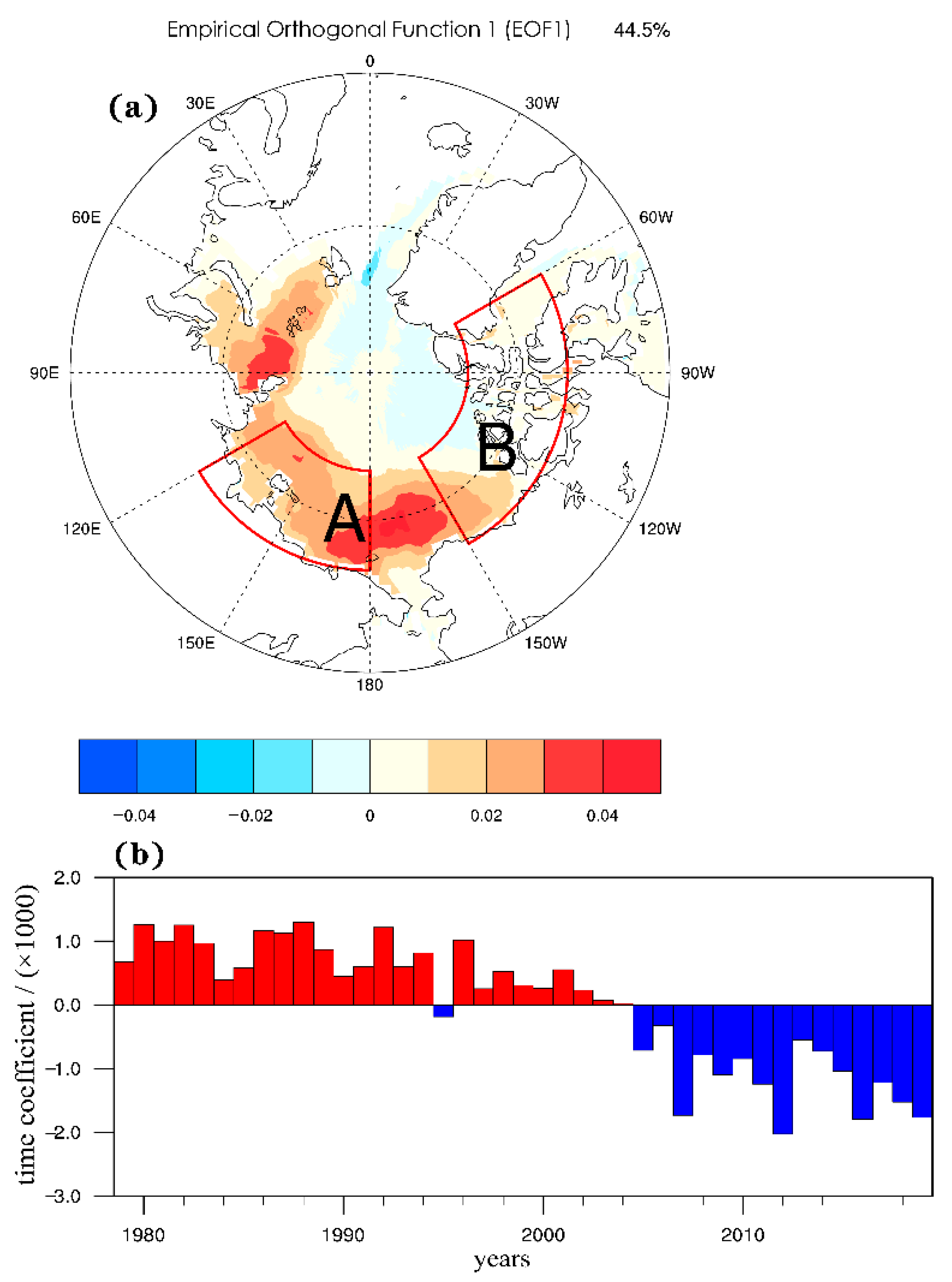
Figure 5.
The lag-related (temperature since September) relation between the sea ice concentration of the Arctic during August to October from 1979 to 2019 and the average temperature in the TP.
Figure 5.
The lag-related (temperature since September) relation between the sea ice concentration of the Arctic during August to October from 1979 to 2019 and the average temperature in the TP.

Figure 6.
Correlation between (a) number of cold days and (b) cold nights over the TP during November to the following February with Arctic sea ice concentration during August to October from 1979 to 2019 (shaded areas are for values that pass the 0.05 significance test), (c) standardized time series of Arctic sea ice concentration during August to October from 1979 to 2019 (the solid black line shows the 9-year moving average curve).

Figure 7.
The regression between cold days during November to the following February and detrend of sea ice concentration in the vital area during August to October (station marking green dots through a 0.05 significance test).
Figure 7.
The regression between cold days during November to the following February and detrend of sea ice concentration in the vital area during August to October (station marking green dots through a 0.05 significance test).

Figure 8.
500 hPa height field differences ((a): 2010c minus CTL. (b): 2090c minus CTL. unit: dagpm. The black net areas passed the 0.05 significance level test).
Figure 8.
500 hPa height field differences ((a): 2010c minus CTL. (b): 2090c minus CTL. unit: dagpm. The black net areas passed the 0.05 significance level test).
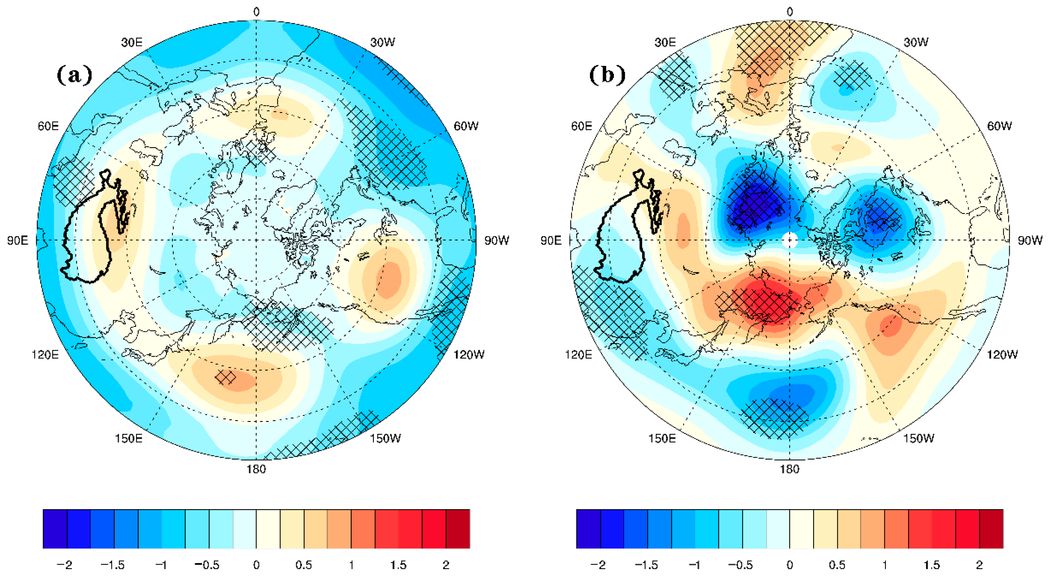
Figure 9.
500 hPa horizontal wind field differences ((a): 2010c minus CTL. (b): 2090c minus CTL. unit: m s−1, the shaded region passed the 0.05 significance level test).
Figure 9.
500 hPa horizontal wind field differences ((a): 2010c minus CTL. (b): 2090c minus CTL. unit: m s−1, the shaded region passed the 0.05 significance level test).

Figure 10.
The differences of 70°–110° E average latitude circulation (unit: m s−1) and temperature (shading, unit: °C) ((a): 2010c minus CTL. (b): 2090c minus CTL, the black shading is terrain).
Figure 10.
The differences of 70°–110° E average latitude circulation (unit: m s−1) and temperature (shading, unit: °C) ((a): 2010c minus CTL. (b): 2090c minus CTL, the black shading is terrain).

Figure 11.
Atmospheric thickness differences of 950–500 hPa (unit: dagpm. (a): 2010c minus CTL. (b): 2090c minus CTL, the white shading is where no data are available).
Figure 11.
Atmospheric thickness differences of 950–500 hPa (unit: dagpm. (a): 2010c minus CTL. (b): 2090c minus CTL, the white shading is where no data are available).

Figure 12.
The differences of EP flux (vector, unit: kg s−2) and the divergence (shading, unit: m s−1 d−1) on the average wave 4–7 at 70°–110° E ((a): 2010c minus CTL, (b): 2090c minus CTL, the black shading is terrain).
Figure 12.
The differences of EP flux (vector, unit: kg s−2) and the divergence (shading, unit: m s−1 d−1) on the average wave 4–7 at 70°–110° E ((a): 2010c minus CTL, (b): 2090c minus CTL, the black shading is terrain).


Table 1.
Definition of cold indices of extreme temperature.
| Cold Index of Extreme Temperature | Definition (Unit: Day) |
|---|---|
| The number of cold days (TX10P) | Days with daily maximum temperature less than 10% percentile (The quantile is based on the period from 1981 to 2010) |
| The number of cold nights(TN10P) | Days with daily minimum temperature less than 10% percentile (The quantile is based on the period from 1981 to 2010) |
Publisher’s Note: MDPI stays neutral with regard to jurisdictional claims in published maps and institutional affiliations. |
© 2022 by the authors. Licensee MDPI, Basel, Switzerland. This article is an open access article distributed under the terms and conditions of the Creative Commons Attribution (CC BY) license (https://creativecommons.org/licenses/by/4.0/).
Share and Cite
MDPI and ACS Style
Jiao, Y.; Zhang, Y.; Hu, P. Can Arctic Sea Ice Influence the Extremely Cold Days and Nights in Winter over the Tibetan Plateau? Atmosphere 2022, 13, 246. https://doi.org/10.3390/atmos13020246
AMA Style
Jiao Y, Zhang Y, Hu P. Can Arctic Sea Ice Influence the Extremely Cold Days and Nights in Winter over the Tibetan Plateau? Atmosphere. 2022; 13(2):246. https://doi.org/10.3390/atmos13020246
Chicago/Turabian StyleJiao, Yang, Yuqing Zhang, and Peng Hu. 2022. "Can Arctic Sea Ice Influence the Extremely Cold Days and Nights in Winter over the Tibetan Plateau?" Atmosphere 13, no. 2: 246. https://doi.org/10.3390/atmos13020246
Note that from the first issue of 2016, this journal uses article numbers instead of page numbers. See further details here.