Article

Investigating Vertical Distributions and Driving Factors of Black Carbon in the Atmospheric Boundary Layer Using Unmanned Aerial Vehicle Measurements in Shanghai, China

1
Center for Intelligent Transportation Systems and Unmanned Aerial Systems Applications, School of Naval Architecture, Ocean and Civil Engineering, Shanghai Jiao Tong University, Shanghai 200240, China
2
Merchant Marine College, Shanghai Maritime University, Shanghai 201306, China
*
Author to whom correspondence should be addressed.
Atmosphere 2023, 14(10), 1472; https://doi.org/10.3390/atmos14101472
Submission received: 26 August 2023 / Revised: 20 September 2023 / Accepted: 21 September 2023 / Published: 23 September 2023
(This article belongs to the Special Issue Urban VOC Emission, Transport, and Chemistry (VOC/ETC))

Abstract

:
Black carbon (BC) is a significant component of fine particulate matter (PM2.5, with aerodynamic diameters ≤ 2.5 μm), and its spatial distribution greatly affects the global radiation budget. However, the vertical distributions and key driving factors of BC in the atmospheric boundary layer, where BC is mostly concentrated, remain unclear. In this study, gradient measurements of BC were made using an unmanned aerial vehicle (UAV) platform from ground level to 500 m above ground level (AGL) during and after the 2016 G20 control period in Shanghai. Generally, vertical profiles of BC from local time (LT) 9 to 17 on all experimental days demonstrated an upward trend with increasing height. The BC emitted from chimneys was initially released at higher altitudes, resulting in the positive gradients of vertical BC profiles. Furthermore, with the progressive development of the boundary layer height from LT 9 to 15, the average concentration of BC per vertical profile decreased. However, meteorological conditions unfavorable for dispersions caused by particularly high temperatures, low wind speed, unfavorable boundary layer conditions, or especially high relative humidity, and hygroscopic growth owing to the extremely high relative humidity, led to an overall increase in vertical BC and ground-based PM2.5 and BC. Despite the impact of adverse meteorological conditions, emission control measures during the control period not only effectively decreased the BC concentration but also reduced the proportion of BC in PM2.5 in the atmospheric boundary layer. The results of this study can provide valuable observations for evaluating numerical model results and important implications for making control strategies of BC in the future.

1. Introduction

Owing to the strong economic development for the last few decades, China has experienced severe and persistent haze pollution [1,2,3]. BC, also referred to as soot, is an essential component of PM2.5. When compared to the total mass of PM2.5, BC contributes a fraction of about 5–15% to the total aerosol mass concentration in urban air [4]. However, BC is an important particulate pollutant because of its adverse health impacts [5,6,7]. Anthropogenic sources of BC derive from the incomplete combustion of fossil fuels and biomass burning. As a result, some toxic and hazardous materials such as polycyclic aromatic hydrocarbons absorbed on the surface of BC are carcinogenic, teratogenic, and mutagenic when inhaled. Additionally, BC plays a unique and important role in global climate change [8,9,10,11,12]. BC has been proved to be the second most vital warming element after carbon dioxide in the global atmospheric system [13]. The strong absorption of a wide range of solar radiation by BC has a great potential to exacerbate global warming. As a byproduct of the incomplete combustion process, BC is typically in the fine submicron size range and is initially hydrophobic [14]. Therefore, BC has a long atmospheric lifetime, allowing it to be transported to higher regions of the atmosphere, both horizontally and vertically [15]. Until now, most studies focusing on the surface-level characteristics of BC have revealed the urgent need to investigate the vertical variation of BC in order to better understand its indirect climate impact and improve model simulations [16].
Vertical profiles of BC in previous studies were obtained using towers, aircraft, tethered/free-flying balloons, and UAVs. Sun et al. (2020) [17] obtained vertical profiles of BC using a 356 m meteorological tower in Shenzhen in December 2017. Generally, BC decreased with increasing height. Zhao et al. (2015) [18] recorded vertical profiles of BC by using aircraft measurements around Beijing between April and June 2012. Generally, BC decreased with increasing height within 1000 m. Li et al. (2015) [16] measured vertical profiles of BC using a tethered balloon within 1000 m in Shanghai in December 2013. In the morning, BC profiles decreased with increasing height. During noon and afternoon, BC profiles were homogenously distributed with height. In the early evening and late evening, BC profiles first decreased with increasing height, and then increased with increasing altitude. Lu et al. (2019) [19] acquired vertical profiles of BC using a tethered balloon within 1000 m in Shouxian from 14 December 2016 to 4 January 2017. Four profile types were categorized: I: uniform vertical distributions (38%, mainly occurring during the periods of 11:00–17:00), II: higher values at lower altitudes (29%, mainly occurring from 20:00 to 8:00 the following day), III: bimodal distributions with high values near the ground and at higher altitudes (17%, mainly occurring around midnight), and IV: unimodal distributions with high values at higher altitudes (11%, mainly occurring during the periods of 11:00–17:00). Liu et al. (2020) [20] measured vertical profiles of BC using a UAV within 500 m in Macau during February and March 2018. In general, BC decreased with increasing height. Wu et al. (2021) [21] measured vertical profiles of BC using a UAV within 900 m in Shenzhen in December 2017 and August 2018. Generally, BC decreased with increasing height.
The eleventh international forum for the governments and central bank governors from 20 major economies, known as the G20 Summit, was held in Hangzhou, China on 4–5 September 2016. This was one of the most important international events for China. In order to improve air quality during the 2016 G20 Summit, stringent emission control measures were implemented in Hangzhou and its surrounding cities by the Chinese government before and during the summit. Considering the impact of regional transport, diverse control intensities were adopted in Hangzhou and its surrounding areas. The surrounding areas were divided into the core control area, the strict control area, and the general control area according to the distances of 50 km, 100 km, and 300 km, respectively, from the Hangzhou International Expo Center, which was the main venue of the 2016 G20 Summit [22]. Shanghai, whose downtown was about 162 km northwest of the main venue, was under the general control area. A “G20 Blue” program was put into effect in Shanghai from 24 August to 6 September in 2016. The 14-day emission control scheme consisted of halting or curbing production in factories, traffic restriction, and so on [23]. As one of the most important chemical industry bases in Shanghai, Jinshan District is located in the southwest of the city and is close to the north shore of Hangzhou Bay. Hence, strict emission control measures were adopted in Jinshan District during the 14-day control period.
To evaluate the effects of these short-term emission control actions on air quality improvements during the 2016 G20 Summit, some studies, including in situ observation and model simulation, have been conducted [22,23,24,25,26,27]. Su et al. (2017) [24] monitored vertical profiles of ozone (O3) concentration from 25 August to 18 September 2016 in Hangzhou and found that meteorological conditions instead of short-term control measures dominated the variations in O3 concentration. Zhao et al. (2017) [25] analyzed the ground-based concentration of air pollutants including PM2.5, inhalable particles (PM10), sulfur dioxide (SO2), nitrogen dioxide (NO2), carbon monoxide (CO), and O3 from 24 August to 6 September 2015 and 2016 in Hangzhou and its surrounding regions, and detected that safeguard measures were effective in improving air quality in Hangzhou and its surrounding cities during the summit. Ji et al. (2018) [22] reported the in situ observations of aerosol chemistry and gaseous precursors from 15 August to 12 September, 2016 in Hangzhou, and discovered that short-term control strategies contributed to suppressing particulate pollution while regional transport may counteract the effects of the control strategies to a certain extent. Wu et al. (2019) [26] analyzed the concentration of six air pollutants (PM2.5, PM10, O3, NO2, SO2, and CO) from five monitoring sites and the chemical compositions of PM2.5 from the meteorological station in Hangzhou from 24 August to 6 September 2016 and previous years. The results showed that the air quality in Hangzhou improved dramatically after the implementation of stringent pollution control measures. Li et al. (2019) [23] examined the concentration of atmospheric pollutants and chemical composition of PM2.5 from two supersites in Shanghai from 24 August to 6 September 2014, 2015, and 2016, and found that pollutant levels were significantly reduced resulting from the implementation of strict control measures. Zheng et al. (2019) [27] carried out in situ experiments on atmospheric volatile organic compounds (VOCs) at two supersites in Shanghai from 24 August to 15 September, 2016, and suggested emissions reduction from industrial sources contributed greatly to lowering the abundance and reactivity of VOCs. However, up to now, no studies have been published on the vertical profiles of BC to evaluate the effects of implementing strict emissions controls.
The 2016 G20 Summit offered a great chance to study the impacts of man-made emissions on air quality. In this study, the UAV-based platform was employed to acquire vertical profiles of BC concentration on 24–25 August and 12–13 September 2016 in Jinshan District, Shanghai. The four-day analysis of data measured with the UAV was conducted during and after the 2016 G20 controlled period to analyze the vertical profiles of BC from ground level to 500 m AGL under the joint effect of emissions reduction measures and meteorological factors. The findings of this study can offer significant insights for assessing the accuracy of numerical models and offer crucial guidance for devising future BC control strategies.

2. Materials and Methods

2.1. Experimental Site and UAV Platform

The experimental site of this study is located in Langxia Town, Jinshan District, Shanghai, China, as indicated in Figure 1. Adjacent to Zhejiang Province, Langxia Town is situated in the southwest of central Jinshan District in Shanghai and is approximately 60 km from the city center. As one of the most essential chemical industry bases in Shanghai, Jinshan District was considered a strictly controlled area by the Shanghai Municipal Bureau of Ecology and Environment from 24 August to 6 September 2016 [28]. The Jinshan District primarily encompasses three major industrial zones: the Jinshan Industrial Zone, the Jinshan No. 2 Industrial Zone, and the Shanghai Chemical Industry Park. Numerous chemical parks, petrochemical factories, and power plants are densely concentrated within the boundaries of Jinshan District [29]. As shown in panel A of Figure 1, the experiment site is approximately 110 km northeast of the main venue of the 2016 G20 Summit in Hangzhou. Additionally, as demonstrated in panel B of Figure 1, the site is approximately 15 km west of the Jinshan Industrial Zone and approximately 12 km northwest of the Jinshan No. 2 Industrial Zone. In order to achieve ultra-low emissions during the 2016 G20 control period, two coal-fired power plants located in the Jinshan Industrial Zone and the Jinshan No. 2 Industrial Zone were required to utilize low-sulfur coals, standardize the operation of flue gas treatment facilities, and limit production by 30%. To strictly control the emissions of unorganized organic waste gas in the chemical industries, some enterprises in the Jinshan No. 2 Industrial Zone implemented production suspension, and some enterprises implemented production limitation [30].
The UAV platform consisted of two major parts. The six-rotor UAV, powered by six portable batteries, acted as the carrier. Additionally, a metal cabin was self-designed to carry the portable monitoring instruments needed, which was securely installed underneath the UAV. The UAV had a built-in GPS recording the location and height of the UAV during the experiment’s every second. Moreover, miniature sensors were also placed inside the cabin under the UAV to collect data on PM2.5, BC, meteorological factors (including temperature and relative humidity (RH)), and other pollutants. The mass concentration of PM2.5 was measured using a personal aerosol monitor (mode AM510, TSI, Shoreview, MN, USA). The mass concentration of BC was measured using a microAeth (mode AE51, AethLabs, San Francisco, CA, USA), whose measurement principle was to measure the rate of change in absorption of transmitted light at 880 nanometers caused by continuous collection of aerosol deposit on the filter [31]. The AM510 and AE51 logged the concentration of PM2.5 and BC every second, respectively. Inside the cabin, there was also a temperature and RH data logger (mode HOBO U12-011, Onset, Bourne, MA, USA). The U12-011 data logger was used to collect instantaneous temperature and RH data every second. Additionally, to minimize the interference caused by factors such as flying speed and the rotors of the UAV, the air inlets of the AM510 and AE51 aerosol monitor were positioned above the UAV [32,33].

2.2. Experimental Design and Data Analysis

To assess the effects of emission control measures on BC, the total research period was divided into two stages. In 2016, 24–25 August and 12–13 September were defined as “control period” and “normal period”, respectively. The normal period was the reference stage without emission control measures, while the control period was the stage with stringent pollution control measures. Here, the UAV platform was used to collect vertical profiles of BC. The UAV was controlled to ascend at a steady speed of 2 m·s−1 from the ground level and was kept hovering for one minute every 50 m until 500 m, and then descended at the same steady speed without hovering. Considering the limit of battery capacity and flight safety, 2 m·s−1 was the proper speed for ascending and descending, and 1 min was the suitable hovering period to obtain enough BC concentration samples. All the data for different flights, as indicated in Table 1, were averaged at the same height during every hovering period, ensuring that the results were accurate and reliable. As the UAV was battery-powered, the flying area was not affected by the output of the UAV. However, the air flow was disturbed by the UAV during the period of ascension. For this reason, the data from the descending process are not used in this study.
To ensure the quality and reliability of the experiments, all devices were calibrated before the beginning of each experiment. To obtain a full picture of vertical profiles of BC, the pocket-sized AE 51 used under the UAV was taken to the Pudong environmental monitor station and compared with a standard instrument (mode Aethalometer AE31, Magee Scientific, Berkeley, CA, USA). As indicated by panel A of Figure 2, a 44 h continuous comparison was conducted between the AE51 and AE31 on one-hour averages, and the results showed a linear association between the AE51 and AE31 data (y = 1.69×x − 0.01, R2 = 0.88). The results indicated that measured values of AE51 were almost 1.7 times those measured using AE31; the difference was attributed to different aerosol deposition velocities and mass attenuation cross-section parameters of the two instruments [34]. The comparison results indicated that AE51 was suitable for collecting BC data during the flight period. To acquire surface and vertical profiles of BC, two identical devices (AE51) were equipped on the ground and under the UAV simultaneously to collect BC data. The ground-level AE51, hourly measuring ground-level BC, was fixed on a tripod and was approximately 1.5 m above the ground. The data from the two devices were compared on the ground before the UAV experiments started on 24 August 2016. As presented in panel B of Figure 2, the results indicate that the average values and standard deviations of BC concentration were 2.35 ± 0.45 and 2.32 ± 0.47 μg·m−3 for UAV-based AE51 and ground-based AE51, respectively.
In this study, meteorological data consisted of planetary boundary layer height (PBLH), atmospheric stability, wind speed, wind direction, T, and RH. Hourly background PM2.5 and meteorological parameters including wind speed, wind direction, T, and RH, were derived from a local atmospheric environment monitoring station located in Langxia Town and within 100 m of the experiment site. Additionally, PBLH and atmospheric stability were acquired from the website of the Air Resource Laboratory (https://www.ready.noaa.gov/archives.php (accessed on 20 September 2023)). Additionally, clusters of the 72 h backward trajectories at the height of 10 m were computed to identify the origins of air masses on 24–25 August and 12–13 September 2016, using the HYSPLIT Trajectory Model [35,36]. The model utilized meteorological parameters from the Global Data Assimilation System with a 1-degree global resolution. Conventional observations of wind speed, cloud amount, light intensity, and other factors were employed by Pasquill [37] to classify atmospheric stability conditions into seven dispersion levels, labeled as A (extremely unstable), B (unstable), C (weakly unstable), D (neutral), E (weakly stable), F (stable), and G (extremely stable), respectively.

3. Results and Discussion

3.1. General Overview of Surface PM2.5, BC, and Meteorological Parameters

In 2016, the four-day hourly background PM2.5 and meteorological parameters (including PBLH, atmospheric stability, wind speed, wind direction, temperature, and RH) during the control period (24–25 August) and the normal period (12–13 September) were illustrated in Figure 3. As one of the primary chemical constituents of PM2.5 [38,39], the hourly ground-level BC during the drone flight time period (from LT 9 to 18 on 24 August and from LT 9 to 17 on 25 August) is also presented in panel A1 of Figure 3 for the purpose of comparison. However, the hourly measurement of ground-level BC could not be achieved during the normal period due to equipment failure of the ground-based AE51. On the whole, the 24 h average background PM2.5 during the control period (33.13 μg·m−3 on 24 August and 33.18 μg·m−3 on 25 August) was significantly lower than those during the normal period (47.92 μg·m−3 on 12 September and 46.13 μg·m−3 on 13 September). It was noteworthy that the PM2.5 at LT 6 and 7 on 13 September surpassed the Chinese National Ambient Air Quality Standards (75 μg·m−3), as indicated by the blue dotted line in panels A1 and B1 of Figure 3. Additionally, the average ground-level BC was lower on 25 August (0.99 μg·m−3) than on 24 August (1.87 μg·m−3). This implies that the effect of emission control actions played a positive role in reducing PM2.5 and BC concentration at ground level.
As presented in panel A1 of Figure 3, the variation tendency of ground-level BC was in perfect accord with background PM2.5 on 24 August. The comparison between ground-level PM2.5 and BC is illustrated in Figure 4. As presented in panel A1 of Figure 4, the linear relationship (y = 0.03*x + 0.64, R2 = 0.79) between PM2.5 and BC on 24 August was remarkably similar to that found in a previous study (y = 0.031*x − 0.63, R2 = 0.74) [40], and the powerful correlation coefficient (R2 = 0.79) on 24 August showed that ground-level PM2.5 and BC were highly likely to originate from the same emission sources. However, the situation was exactly the opposite on 25 August, as indicated in panel A1 of Figure 3 and panel A2 of Figure 4. The significantly negative linear correlation between PM2.5 and BC concentration on 25 August showed that air masses entering on 25 August possessed a low concentration of BC at ground level, which was evidenced by the BC/PM2.5 ratios. As displayed in panels A2 and B2 of Figure 4, the BC/PM2.5 ratios at ground level were obtained during the control period. The highest BC/PM2.5 ratio, recorded at LT 9 on both 24 August and 25 August was 0.069 and 0.067, respectively. Clearly, the maximum BC/PM2.5 ratio on both days was extremely similar, which was likely caused by traffic emissions during the morning rush hour, because the road to the parking lot was close to the experimental location of ground-level AE51. On 24 August, the BC/PM2.5 ratios varied from 0.036 to 0.055 from LT 10 to 18, and there was an obviously increasing trend in the BC/PM2.5 ratios from LT 12 to 18. Contrarily, on 25 August, the range of the BC/PM2.5 ratios was between 0.012 and 0.038 from LT 10 to 17, and the BC/PM2.5 ratios exhibited a significantly declining tendency from LT 10 to 14. Additionally, the average BC/PM2.5 ratio from LT 9 to 17 on 24 August (0.044) was 1.64 times higher than the corresponding average ratio on 25 August (0.027). As displayed in Figure 5, the air masses from LT 9 to 17 on 24 August and 25 August indeed derived from distinct clustering categories. The air mass from LT 9 to 17 on 24 August was part of cluster 1, while the air mass from LT 9 to 17 on 25 August belonged to cluster 3. As a result, the proportion of BC in PM2.5 within the air mass of cluster 3 was lower than that within the air mass of cluster 1.
As presented in panel A1 of Figure 3, on 24 August, the PM2.5 continued to rise from LT 9 to 14, reaching a peak value of 60 μg·m−3 at LT 14, and then dropped rapidly from 60 μg·m−3 at LT 15 to 29 μg·m−3 at LT 18. Meanwhile, the BC also demonstrated an increasing tendency from LT 9 to 16, peaking at a maximum value of 2.498 μg·m−3 at LT 16, and then rapidly decreased to 1.582 μg·m−3 at LT 18. On 25 August, the PM2.5 had an increasing trend from LT 9 to 14, reaching a peak value of 50 μg·m−3 at LT 14, and then remained at approximately 48 μg·m−3 from LT 15 to 17. At the same time, the BC significantly decreased from 1.734 μg·m−3 at LT 9 to 0.609 μg·m−3 at LT 14, followed by a gradual increase until LT 17. As presented in panel B1 of Figure 3, on 12 September, the PM2.5 exhibited a considerable decline from LT 8 to 10, then gradually decreased to LT 14, and eventually had a slight increase at LT 17 and 18. On 12 September, there was also a rapid decline in PM2.5 from LT 8 to 9, subsequently followed by a gradual decrease until LT 15, and ultimately increased until LT 18. Notably, the PM2.5 peaked at around LT 14 on 24–25 August, whereas the PM2.5 reached its lowest point at approximately LT 15 on 12–13 September. As illustrated in Figure 5, 72 h backward trajectories during the control and normal period were grouped by clusters. The averaged PM2.5 were 36.72 μg·m−3 for cluster 1, 30.79 μg·m−3 for cluster 2(1), 54.60 μg·m−3 for cluster 2(2), 38.63 μg·m−3 for cluster 3, and 43.58 μg·m−3 for cluster 4, respectively. According to the Chinese National Ambient Air Quality Standards, air masses were considered polluted when the PM2.5 concentration exceeded 75 μg·m−3. Generally, the average PM2.5 was less than 75 μg·m−3 in all clusters. Therefore, there were no significant local emissions or long-range transmission of pollutants during the control and normal periods. It is a well-established fact that local emissions significantly reduced during the control period, whereas no such restrictions were imposed during the normal period. The air masses of cluster 2(1) and cluster 2(2) originated from the same direction, but the average PM2.5 for cluster 2(1) (30.79 μg·m−3) was lower than that for cluster 2(2) (54.60 μg·m−3), which was probably due to local emission reduction during the control period.
In general, meteorological parameters contribute greatly to air pollutant concentration changes in addition to local emission intensities and long-range transmission of pollutants [1]. PBLH is a particularly important factor, as it impacts the vertical diffusion of air pollutants through turbulence [41]. As presented in panel B3 of Figure 3, the height of the boundary layer surpassed 500 m from LT 8 to 17 on 12–13 September. Furthermore, the dispersion and accumulation of pollutants can be substantially influenced by atmospheric stability [20]. As illustrated in panel B3 of Figure 3, the atmospheric stability was predominantly C (weakly unstable) from LT 8 to 17 on 12–13 September, conducive to the dispersion of pollutant concentrations. In addition, the average wind speed from LT 8 to 17 was 2.91 m·s−1 and 3.06 m·s−1 on 12 September and 13 September, respectively. These wind speeds were faster than the average wind speed during other time periods on the same days (1.34 m·s−1 and 1.25 m·s−1 on 12 September and 13 September, respectively). Consequently, as a result of the cumulative effects of an unstable atmospheric condition, a well-developed boundary layer height, and augmented wind speed, the PM2.5 attained its minimum level at approximately LT 15 on both 12 September and 13 September. Additionally, the average PM2.5 from LT 8 to 17 on 12 September and 13 September was 38 μg·m−3 and 37 μg·m−3, respectively. These values were notably lower than the average PM2.5 observed during other time periods on the same days (55 μg·m−3 and 53 μg·m−3 on 12 September and 13 September, respectively). However, as illustrated in panels A3 and B3 of Figure 3, the atmospheric stability was primarily D (neutral) from LT 8 to 17 on 24–25 August, which was found to be more stable in comparison to 12–13 September. Worse still, the average temperatures from LT 8 to 18 on 24 August and 25 August were 34.58 °C and 35.20 °C, respectively. These temperatures were approximately 5 °C higher than the average temperature during the same period on 12 September (29.35 °C) and 13 September (28.99 °C). Generally, particularly high temperatures and low wind speed in summer tend to enhance the stability of the atmosphere, thereby hindering the dispersion and dilution of pollutants [42]. Obviously, the temperatures exceeded 35 °C from LT 11 to 15 on 24 August, and the wind speed remained relatively low during the same period. Therefore, it was highly probable that the peak PM2.5 concentration at LT 14 on 24 August was due to meteorological conditions unfavorable for dispersion, which were caused by the particularly high temperatures and relatively low wind speeds. Following the decrease in temperatures and the increase in wind speeds after LT 16 on 24 August, the PM2.5 began to decline. As demonstrated in Figure 6, the variation in PM2.5 on 25 August was the least significant compared to the other three days. This also indicated that, in comparison to the remaining three days, the atmospheric condition on 25 August was the most stable. Like 24 August, the peak PM2.5 concentration was 50 μg·m−3 at LT 14 on 25 August. Nevertheless, the boundary layer height on 25 August dropped rapidly from 1236 m at LT 14 to 255 m at LT 17. Additionally, the PM2.5 remained approximately 49 μg·m−3 from LT 14 to 17 on 25 August, despite the increased wind speeds. As a result, the higher PM2.5 between LT 14 and 17 on 25 August was attribute to meteorological conditions unfavorable for dispersion, which were caused by the particularly high temperatures and unfavorable boundary layer condition. However, the decrease in black carbon concentration on 25 August was probably due to the reduction in local emission sources and the external air masses from the sea having low black carbon concentration.

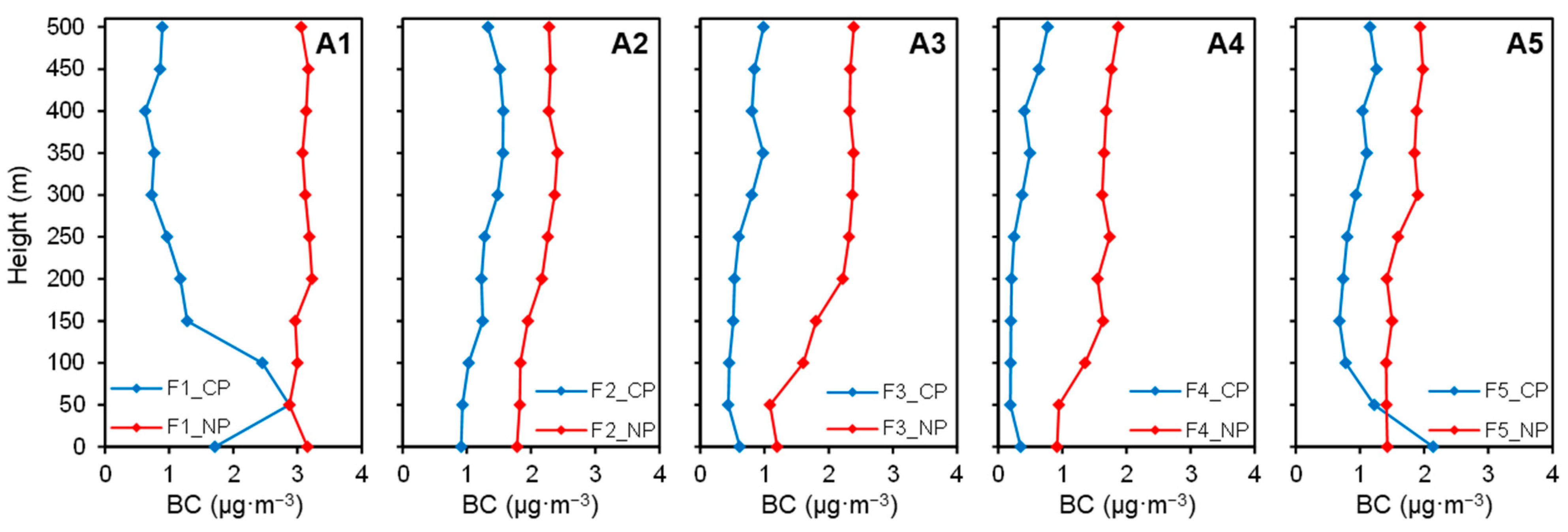
3.2. Vertical Distribution of BC

As presented in Table 1, the UAV-based platform successfully completed a total of twenty vertical observation missions from LT 8 to 17 on both 24–25 August and 12–13 September, 2016. Within this group, a total of ten effective vertical observation flights were completed during the control period (24–25 August) of environmental air quality guarantee measure implementation, while an additional ten effective vertical observation flights were conducted during the normal period (12–13 September) when these guarantee measures were not in place. The BC was averaged every 50 m until 500 m, with the UAV hovering for one minute at each of these heights during every flight. As demonstrated in panels A3 and B3 of Figure 3, the altitude of the atmospheric boundary layer consistently exceeded the maximum flight altitude of the UAV (500 m) during the period of drone experiments, except for LT 17 on 25 August. However, the fifth flight on 25 August was conducted around LT 17. As presented in Figure 7 and Tables S1 and S2, vertical profiles of BC and meteorological parameters (including temperature and RH) were measured using the UAV during the control period. August 24 marked the commencement of pollution reduction measures, with 25 August serving as the subsequent day of their implementation.
On 24 August, the BC of the first UAV flight decreased by 60% from 2.113 μg·m−3 at ground level to 0.843 μg·m−3 at 100 m AGL, and then the BC fluctuated around 0.750 μg·m−3 between 100 and 500 m AGL, accompanied by a minor downward tendency. Between LT 8 and 9, it was highly probable that the elevated BC concentration in the vicinity of the ground was attributable to traffic emissions during the morning rush hour, because the road to the parking lot was close to the drone’s launch site. This conclusion agreed well with a previous study [16] conducted in Fengxian District, Shanghai. During the second UAV flight, the BC was mixed uniformly from ground level to 500 m AGL due to the development of the boundary layer, with a slight upward trend. Similar to the second flight, an increasing trend was also observed in the BC of the third UAV flight. Nonetheless, the upward trend of the third flight was more significant, with an ascent gradient of 0.111 μg·m−3 per 50 m. In previous studies [16,20], the BC decreased with increasing height within the boundary layer height. However, the trend of BC with altitude in this study was different from that reported in previous studies. Given the fact that, although the factory production was reduced at this time, the BC emitted from chimneys was initially released at a higher altitude, resulting in an increase in BC concentration in the air. Additionally, the BC on the fourth UAV flight experienced an overall rise from ground level to 500 m AGL, notwithstanding the fact that the fourth flight was conducted under the most favorable boundary layer conditions. Like the variations observed in background PM2.5 around LT 14 on 24 August, the overall rise in temperatures during the fourth flight as presented in panel A2 of Figure 7 probably led to adverse meteorological conditions, which resulted in the increased BC concentration, despite the reduction in local emissions and the absence of long-range transport of pollution. As shown in Table S1, the PM2.5 concentration was also higher in the fourth flight. During the fifth UAV flight, the BC decreased by 59% from 2.100 μg·m−3 at ground level to 0.868 μg·m−3 at 100 m AGL, and the positive gradient of BC concentration from 150 to 500 m AGL was 0.123 μg·m−3 per 50 m. Similarly to the first flight, traffic emission during the evening rush hour was also probably responsible for the rise in BC concentration from ground level to 100 m AGL during the fifth flight.
On 25 August, the BC of the first UAV flight demonstrated a general downward trend, except for notably high values at 50 and 100 m AGL. As the boundary layer height developed, the pollution caused by traffic emissions during the morning rush hour was elevated. The BC in the second flight, third flight, and fourth flight all showed a slight increasing trend with increasing altitude. With the progressive development of the boundary layer height, the overall BC concentration in the second flight, third flight, and fourth flight gradually decreased. As presented in panel B3 of Figure 3, as the boundary layer continuously rose from LT 8 to 14, the atmospheric stability varied from E (weakly stable) to C (weakly unstable). As a result, the less stable the atmospheric stability, the lower the BC concentration was. This is because, when the atmospheric stability was less stable, the turbulence was more intense, making it easier for pollutants to be diluted and dispersed [43]. Additionally, the slight inversion presented below 100 m AGL on 25 August did not produce a significant impact on the BC concentration. This was probably attributed to the thinner and more rapid dissipation of inversion layers during summer. Like on the 24 August, the BC in the fifth UAV flight on 25 August decreased by 64% from 2.141 μg·m−3 at ground level to 0.779 μg·m−3 at 100 m AGL, and the BC showed a slight increasing trend from 150 to 500 m AGL. Similarly, traffic emissions during the evening rush hour could also be a contributing factor to the increased BC concentration below 100 m AGL in the fifth UAV flight. It was worth noting that the overall BC concentration for the fifth flight on 25 August was significantly higher than that of the third and fourth flights. As illustrated in panel A3 of Figure 3, this was potentially caused by the steep drop in the height of the boundary layer from LT 14 to 17. As presented in Table S2, the PM2.5 concentration was also higher in the fifth flight.
As illustrated in Figure 8, a comprehensive comparison of the BC for each individual flight mission monitored by drones on 24 August and 25 August was presented, with the influence of traffic emissions during rush hours being excluded from the analysis. It was observed that the average BC for the second flight, third flight, and fourth flight on 25 August were, respectively 26%, 54%, and 85% lower than those recorded on 24 August. Compared to other flights, the average BC in the fourth flight on 24 August was particularly high, which was probably due to adverse meteorological conditions, which were caused by the overall rise in temperatures during the fourth flight. Nevertheless, after excluding the impact of traffic emissions, the average BC for the fifth flight on 25 August only decreased by 0.102 μg·m−3 in comparison to that on 24 August, while the BC for the first flight on 25 August was unexpectedly found to increase by 0.162 μg·m−3 compared to that on 24 August. Obviously, stable meteorological conditions on 25 August probably obstructed the dispersion of BC for the first and fifth flight.
As presented in Figure 9 and Tables S3 and S4, vertical profiles of BC and meteorological parameters (including temperature and RH) during the normal period were measured with the UAV. On 12 September, the BC from the ground to 500 m AGL for the first flight was mixed uniformly, with small-scale fluctuations around 3.598 μg·m−3. Additionally, the BC in the first flight demonstrated a slight increasing trend with height. The variation trend of BC in the second flight was similar to that of the first flight. However, the average BC concentration for the first flight was 36% higher than that for the second flight, which is probably attributable to unfavorable atmospheric dispersion conditions and hygroscopic growth, which were both likely caused by the extremely high RH (72–84%) experienced during the first flight. As indicated in the previous study [44], regardless of hydrophilic aerosol particles (such as sulfuric acid, ammonium sulfate, and ammonium nitrate) or hydrophobic aerosol particles (such as sandstorms and black carbon), when the RH is less than 80%, hygroscopic growth is slow; however, when the RH is between 80 and 95%, hygroscopic growth accelerates. In another study [45], two severe pollution processes occurred under weak wind (wind speed ≤ 3 m·s−1) and high relative humidity (≥80%). Additionally, high relative humidity reduces turbulent heat exchange, leading to unfavorable conditions for atmospheric dispersion [46]. As illustrated in Table S3, the PM2.5 concentration was also higher in the first flight. In the third flight, the BC demonstrated a tendency to increase with altitude as well. However, the gradient from ground level to 150 m AGL in the third flight was 0.332 μg·m−3 per 50 m, higher than the gradient from 150 to 500 m AGL (0.048 μg·m−3 per 50 m). The BC in the fourth and fifth flight also showed a minor increasing trend with altitude from ground level to 500 m AGL, with the gradients of 0.065 and 0.062 μg·m−3 per 50 m, respectively. Overall, the average BC concentration progressively diminished from the first flight to the fifth flight on 12 September.
On 13 September, the BC in the first flight decreased from ground to 50 m AGL, then held steady around 2.370 μg·m−3 from 50 to 150 m AGL, and then increased from 150 to 200 m AGL, and finally a slight decrease in the BC concentration was observed between 200 and 500 m AGL. The trends in the changes in BC for the second and third flight exhibited a high degree of similarity. The BC concentration exhibited a slight increasing trend from the ground to 150 m AGL, as well as from 200 to 500 m AGL. Nevertheless, the elevation in BC was more prominent from 150 to 200 m AGL. Moreover, the BC in the fourth flight demonstrated the most significant increasing gradient on 13 September, which was 0.126 μg·m−3 per 50 m. The BC in the fifth flight fluctuated around 1.730 μg·m−3 and 2.177 μg·m−3 from ground to 200 m AGL and from 200 to 500 m AGL, respectively. However, the BC concentration notably increased from 200 to 300 m AGL in the fifth flight. Overall, the concentration of BC on 13 September was primarily concentrated within the range of 1–3 μg·m−3 as presented in panel B1 of Figure 9.

3.3. Effect of Emission Control Actions on Vertical Profiles of BC

Vertical profiles of the BC measured with the UAV were obtained during the control and normal period to evaluate the effects of emission control measures on vertical profiles of BC. As 25 August was the second day of implementation of emission reduction measures, vertical profiles of the BC on 25 August were regarded as samples after implementation of emission reduction measures during control period. Additionally, the average of vertical profiles of BC on 12 September and 13 September were used as samples during the normal period. Vertical profiles of BC during each within the two periods were compared separately. The first to fifth flights were conducted during the control and normal period, specifically from LT 8 to 9, LT 9 to 10, LT 11 to 12, LT 14 to 15, and LT 16 to 17.
As presented in panel A1 of Figure 10, upon exclusion of the effects of traffic emissions, the BC of the first flight from 150 to 500 m AGL during the control period demonstrated a downward trend with increasing altitude. Furthermore, the BC of the first flight during the normal period was uniformly mixed, with minimal fluctuations around 3.086 μg·m−3. During the normal period, the influence of traffic emissions during the morning rush hour on BC concentration was found to be insignificant, because the drone’s launch site during the normal period was situated at a considerable distance from the road leading to the parking lot. Additionally, the average BC of the first flight from 150 to 500 m AGL during the normal period was 3.4 times that during the control period. As illustrated in panel A2 of Figure 10, the variations in BC of the second flight during the control and normal period exhibited a similar pattern, both demonstrating a minor increasing tendency with increasing altitude from ground to 500 m, with the gradient of 0.041 and 0.050 μg·m−3 per 50 m, respectively. Nevertheless, the average BC of the second flight during the normal period was 1.7 times that during the control period. As shown in panels A3 and A4 of Figure 10, the BC for the third and fourth flight during the control and normal period also exhibited an upward trend with altitude. In addition, the upward trend in BC for the third and fourth flight from the ground to 150 m AGL was more pronounced during the normal period. Furthermore, the average BC for the third and fourth flight during the normal period were found to be 2.9 and 4.1 times greater, respectively, than those obtained during the control period. As demonstrated in panel A5 of Figure 10, the BC of the fifth flight during the control period decreased from ground level to 150 m AGL, probably due to the influence of traffic emissions during evening rush hour. Considering the takeoff times of the fifth flight during the normal period were approximately LT 16, and the drone’s launch site was situated at a considerable distance from the road leading to the parking lot, the BC of the fifth flight during the normal period was not influenced by traffic emissions during evening rush hour. The changes in BC from 150 to 500 m AGL for the fifth flight during the control and normal period also demonstrated a slightly increasing trend with increasing altitude, but the average BC from 150 to 500 m AGL for the fifth flight during the normal period was 1.8 times greater than that during the control period. In summary, the emission reduction measures during the control period played a significant role in reducing the BC concentration within 500 m AGL, with the sole exception being the influence of traffic emissions during morning and evening rush hours.
As illustrated in Figure 11, the box diagrams depicted the BC and the BC/PM2.5 ratios for five flights measured using the UAV during the control and normal period, with the influence of rush hours on BC concentration being excluded. Overall, the average BC and the average BC/PM2.5 ratio for the five flights during the normal period were both higher than the corresponding values for the five flights during the control period as presented in Figure 11. This is likely attributable to the primary focus on stringent control on emissions from coal-fired power plants and rigorous coal quality management as key elements in the early stages of emissions reduction efforts in Jinshan District, Shanghai. When unaffected by traffic emissions, the BC/PM2.5 ratios during the control period were primarily distributed within the range of 0.033–0.059. Conversely, when influenced by traffic emissions, the BC/PM2.5 ratios were found to be very high, with a distribution between 0.092 and 0.188. Moreover, the BC/PM2.5 ratios for all flights during the normal period were relatively concentrated, the majority of which fell between 0.063 and 0.075. Therefore, following the exclusion of the effects of traffic emissions during peak hours, the implementation of emission reduction measures during the control period not only effectively mitigated the BC concentration from ground to 500 m AGL but also diminished the proportion of BC in PM2.5. Upon comparison with the BC/PM2.5 ratios (8.0 ± 3.2% in February and 9.6 ± 7.5% in March) in the previous study [20], it was observed that the BC/PM2.5 ratios in the present study were lower. This discrepancy could be attributed to the fact that the previous study was performed during winter, while this study was conducted in summer.

4. Conclusions

UAV-based vertical profiles of BC during and after the 2016 G20 Summit were measured in Jinshan District, Shanghai. In total, twenty vertical observation missions (ten during the control period and ten during the normal period) were presented to analyze gradient measurements of BC from the ground level to 500 m AGL under the joint effect of short-term emission control measures and meteorological factors. In addition, the background PM2.5 and meteorological parameters (including PBLH, atmospheric stability, wind speed, wind direction, temperature, and RH) during the control and normal period were also presented to assess the effect of emission control actions at ground level. Additionally, the hourly ground-level BC during the drone flight time period was also displayed for the purpose of comparison. Furthermore, the ground-level BC/PM2.5 ratios during the control period and UAV-based BC/PM2.5 ratios during the control and normal period were also presented.
On the whole, the average background PM2.5 during the control period was significantly lower than that during the normal period. Additionally, the average ground-level BC on 25 August was lower than that on 24 August. The results imply that the effect of emission control actions played an effective role in reducing pollutant concentration at ground level. The linear relationship between ground-level PM2.5 and BC on 24 August showed that they were highly likely to originate from the same emission sources, but the situation was exactly the opposite on 25 August. After excluding the impact of rush-hour traffic emissions, the BC/PM2.5 ratios on 24 August varied from 0.036 to 0.055, while the range of the BC/PM2.5 ratios was between 0.012 and 0.038 on 25 August. The results of clusters of the 72 h backward trajectories during the control and normal period revealed that there was probably no significant long-range transmission of pollutants. However, the PM2.5 peaked at around LT 14 during the control period was mainly due to meteorological conditions unfavorable for dispersion, which were caused by particularly high temperatures, low wind speed or unfavorable boundary layer conditions.
During the control and normal period, vertical profiles of BC observed from the ground to 500 m AGL from LT 9 to 16 demonstrated a clearly increasing trend with respect to height. This phenomenon was attributable to chimney emissions that were initially released at higher altitudes. The increasing gradient ranged from 0.037 to 0.068 μg·m−3 per 50 m during the control period, and varied from 0.050 to 0.120 μg·m−3 per 50 m during the normal period. Additionally, with the continuous development of the boundary layer height, the average concentration of BC per vertical profile decreased from LT 9 to 15 on all experimental days, except for 24 August. As the average BC in the fourth flight on 24 August was particularly high, which was probably due to adverse meteorological conditions caused by the overall rise in temperatures around LT 14. Additionally, the average BC for the first flight on 12 September was notably high, which was attributable to the unfavorable atmospheric dispersion condition and hygroscopic growth caused by the extremely high RH experienced during the first flight. Overall, the average BC concentration and the average BC/PM2.5 ratio per vertical profile during the normal period were both higher than the corresponding values during the control period, with the influence of traffic emissions during rush hours excluded. Moreover, the vertical BC/PM2.5 ratios of all flights during the control period were primarily distributed within the range of 0.033–0.059, while the majority of the vertical BC/PM2.5 ratios during the normal period were between 0.063 and 0.075. As a result, the implementation of pollution reduction measures during the control period effectively reduced the BC concentration and the proportion of BC in PM2.5 from within the atmospheric boundary layer. These conclusions can provide important insights for estimating the accuracy of numerical models and offer primary guidance for devising future BC control strategies.

Supplementary Materials

The following are available online at https://www.mdpi.com/article/10.3390/atmos14101472/s1, Table S1: The average values and standard deviations of black carbon (BC), PM2.5, temperature (T), and relative humidity (RH) during the UAV flights on August 24, 2016; Table S2: The average values and standard deviations of BC, PM2.5, T and RH during the UAV flights on August 25, 2016; Table S3: The average values and standard deviations of BC, PM2.5, T and RH during the UAV flights on September 12, 2016; Table S4. The average values and standard deviations of BC, PM2.5, T and RH during the UAV flights on September 13, 2016.

Author Contributions

Conceptualization, H.W.; methodology, H.W.; software, H.W.; validation, H.W.; formal analysis, H.W.; investigation, H.W.; resources, H.W. and C.H.; data curation, H.W. and C.H.; writing—original draft preparation, H.W.; writing—review and editing, H.W. and C.H.; visualization, H.W.; supervision, H.W.; project administration, C.H.; funding acquisition, C.H. All authors have read and agreed to the published version of the manuscript.

Funding

This research was funded by the National Science Foundation of China, grant number 51909156.

Institutional Review Board Statement

Not applicable.

Informed Consent Statement

Not applicable.

Data Availability Statement

The data are not publicly available, as the data are part of an ongoing study.

Conflicts of Interest

The authors declare no conflict of interest.

References

  1. Chan, C.K.; Yao, X. Air pollution in mega cities in China. Atmos. Environ. 2008, 42, 1–42. [Google Scholar] [CrossRef]
  2. Ouyang, Y.D. China wakes up to the crisis of air pollution. Lancet Respir. Med. 2013, 1, 12. [Google Scholar] [CrossRef] [PubMed]
  3. Parrish, D.D.; Zhu, T. Clean Air for Megacities. Science 2009, 326, 674–675. [Google Scholar] [CrossRef] [PubMed]
  4. Yang, F.; Tan, J.; Zhao, Q.; Du, Z.; He, K.; Ma, Y.; Duan, F.; Chen, G.; Zhao, Q. Characteristics of PM2.5 speciation in representative megacities and across China. Atmos. Chem. Phys. 2011, 11, 5207–5219. [Google Scholar] [CrossRef]
  5. Pope, C.A.; Ezzati, M.; Dockery, D.W. Fine-Particulate Air Pollution and Life Expectancy in the United States. N. Engl. J. Med. 2009, 360, 376–386. [Google Scholar] [CrossRef] [PubMed]
  6. Bond, T.C.; Doherty, S.J.; Fahey, D.W.; Forster, P.M.; Berntsen, T.; DeAngelo, B.J.; Flanner, M.G.; Ghan, S.; Karcher, B.; Koch, D.; et al. Bounding the role of black carbon in the climate system: A scientific assessment. J. Geophys. Res. -Atmos. 2013, 118, 5380–5552. [Google Scholar] [CrossRef]
  7. Wang, L.J.; Bao, S.Y.; Liu, X.L.; Wang, F.; Zhang, J.W.; Dang, P.Y.; Wang, F.L.; Li, B.; Lin, Y. Low-dose exposure to black carbon significantly increase lung injury of cadmium by promoting cellular apoptosis. Ecotoxicol. Environ. Saf. 2021, 224, 112703. [Google Scholar] [CrossRef]
  8. Jacobson, M.Z. Strong radiative heating due to the mixing state of black carbon in atmospheric aerosols. Nature 2001, 409, 695–697. [Google Scholar] [CrossRef]
  9. Menon, S.; Hansen, J.; Nazarenko, L.; Luo, Y.F. Climate effects of black carbon aerosols in China and India. Science 2002, 297, 2250–2253. [Google Scholar] [CrossRef]
  10. Babu, S.S.; Satheesh, S.K.; Moorthy, K.K. Aerosol radiative forcing due to enhanced black carbon at an urban site in India. Geophys. Res. Lett. 2002, 29, 27-1–27-4. [Google Scholar] [CrossRef]
  11. Babu, S.S.; Moorthy, K.K.; Satheesh, S.K. Aerosol black carbon over Arabian Sea during intermonsoon and summer monsoon seasons. Geophys. Res. Lett. 2004, 31. [Google Scholar] [CrossRef]
  12. Reveillet, M.; Dumont, M.; Gascoin, S.; Lafaysse, M.; Nabat, P.; Ribes, A.; Nheili, R.; Tuzet, F.; Menegoz, M.; Morin, S.; et al. Black carbon and dust alter the response of mountain snow cover under climate change. Nat. Commun. 2022, 13, 5279. [Google Scholar] [CrossRef]
  13. Haywood, J.; Boucher, O. Estimates of the direct and indirect radiative forcing due to tropospheric aerosols: A review. Rev. Geophys. 2000, 38, 513–543. [Google Scholar] [CrossRef]
  14. Cooke, W.F.; Wilson, J.J.N. A global black carbon aerosol model. J. Geophys. Res. -Atmos. 1996, 101, 19395–19409. [Google Scholar] [CrossRef]
  15. Moorthy, K.K.; Babu, S.S.; Sunilkumar, S.V.; Gupta, P.K.; Gera, B.S. Altitude profiles of aerosol BC, derived from aircraft measurements over an inland urban location in India. Geophys. Res. Lett. 2004, 31. [Google Scholar] [CrossRef]
  16. Li, J.; Fu, Q.Y.; Huo, J.T.; Wang, D.F.; Yang, W.; Bian, Q.G.; Duan, Y.S.; Zhang, Y.H.; Pan, J.; Lin, Y.F.; et al. Tethered balloon-based black carbon profiles within the lower troposphere of Shanghai in the 2013 East China smog. Atmos. Environ. 2015, 123, 327–338. [Google Scholar] [CrossRef]
  17. Sun, T.L.; Wu, C.; Wu, D.; Liu, B.; Sun, J.Y.; Mao, X.; Yang, H.L.; Deng, T.; Song, L.; Li, M.; et al. Time-resolved black carbon aerosol vertical distribution measurements using a 356-m meteorological tower in Shenzhen. Theor. Appl. Climatol. 2020, 140, 1263–1276. [Google Scholar] [CrossRef]
  18. Zhao, D.L.; Tie, X.X.; Gao, Y.; Zhang, Q.; Tian, H.J.; Bi, K.; Jin, Y.L.; Chen, P.F. In-Situ Aircraft Measurements of the Vertical Distribution of Black Carbon in the Lower Troposphere of Beijing, China, in the Spring and Summer Time. Atmosphere 2015, 6, 713–731. [Google Scholar] [CrossRef]
  19. Lu, Y.; Zhu, B.; Huang, Y.; Shi, S.S.; Wang, H.L.; An, J.L.; Yu, X.N. Vertical distributions of black carbon aerosols over rural areas of the Yangtze River Delta in winter. Sci. Total Environ. 2019, 661, 1–9. [Google Scholar] [CrossRef]
  20. Liu, B.; Wu, C.; Ma, N.; Chen, Q.; Li, Y.W.; Ye, J.H.; Martin, S.T.; Li, Y.J. Vertical profiling of fine particulate matter and black carbon by using unmanned aerial vehicle in Macau, China. Sci. Total Environ. 2020, 709, 136109. [Google Scholar] [CrossRef]
  21. Wu, C.; Liu, B.; Wu, D.; Yang, H.L.; Mao, X.; Tan, J.; Liang, Y.; Sun, J.Y.; Xia, R.; Sun, J.R.; et al. Vertical profiling of black carbon and ozone using a multicopter unmanned aerial vehicle (UAV) in urban Shenzhen of South China. Sci. Total Environ. 2021, 801, 149689. [Google Scholar] [CrossRef] [PubMed]
  22. Ji, Y.; Qin, X.F.; Wang, B.; Xu, J.; Shen, J.D.; Chen, J.M.; Huang, K.; Deng, C.R.; Yan, R.C.; Xu, K.E.; et al. Counteractive effects of regional transport and emission control on the formation of fine particles: A case study during the Hangzhou G20 summit. Atmos. Chem. Phys. 2018, 18, 13581–13600. [Google Scholar] [CrossRef]
  23. Li, H.W.; Wang, D.F.; Cui, L.; Gao, Y.; Huo, J.T.; Wang, X.N.; Zhang, Z.Z.; Tan, Y.; Huang, Y.; Cao, J.J.; et al. Characteristics of atmospheric PM2.5 composition during the implementation of stringent pollution control measures in shanghai for the 2016 G20 summit. Sci. Total Environ. 2019, 648, 1121–1129. [Google Scholar] [CrossRef]
  24. Su, W.J.; Liu, C.; Hu, Q.H.; Fan, G.Q.; Xie, Z.Q.; Huang, X.; Zhang, T.S.; Chen, Z.Y.; Dong, Y.S.; Ji, X.G.; et al. Characterization of ozone in the lower troposphere during the 2016 G20 conference in Hangzhou. Sci. Rep. 2017, 7, 17368. [Google Scholar] [CrossRef] [PubMed]
  25. Zhao, H.; Zheng, Y.; Wei, L.; Guan, Q.; Wang, Z. Evolution and evaluation of air quality in Hangzhou and its surrounding area during the G20 summit. China Environ. Sci. 2017, 37, 2016–2024. [Google Scholar]
  26. Wu, K.; Kang, P.; Tie, X.; Gu, S.; Zhang, X.L.; Wen, X.H.; Kong, L.K.; Wang, S.H.; Chen, Y.Z.; Pan, W.H.; et al. Evolution and Assessment of the Atmospheric Composition in Hangzhou and its Surrounding Areas during the G20 Summit. Aerosol Air Qual. Res. 2019, 19, 2757–2769. [Google Scholar] [CrossRef]
  27. Zheng, S.S.; Xu, X.F.; Zhang, Y.J.; Wang, L.R.; Yang, Y.F.; Jin, S.G.; Yang, X.X. Characteristics and sources of VOCs in urban and suburban environments in Shanghai, China, during the 2016 G20 summit. Atmos. Pollut. Res. 2019, 10, 1766–1779. [Google Scholar] [CrossRef]
  28. Shanghai Municipal Bureau of Ecology and Environment. G20 Summit Shanghai Environmental Air Quality Protection Plan; Shanghai Municipal Bureau of Ecology and Environment: Shanghai, China, 2016. [Google Scholar]
  29. Cai, C.J.; Geng, F.H.; Tie, X.X.; Yu, Q.O.; An, J.L. Characteristics and source apportionment of VOCs measured in Shanghai, China. Atmos. Environ. 2010, 44, 5005–5014. [Google Scholar] [CrossRef]
  30. Shanghai Jinshan District Environmental Protection Bureau. G20 Summit Shanghai Jinshan District Collaborative Environmental Quality Assurance Plan; Shanghai Jinshan District Environmental Protection Bureau: Shanghai, China, 2016. [Google Scholar]
  31. Hagler, G.S.W.; Yelverton, T.L.B.; Vedantham, R.; Hansen, A.D.A.; Turner, J.R. Post-processing Method to Reduce Noise while Preserving High Time Resolution in Aethalometer Real-time Black Carbon Data. Aerosol Air Qual. Res. 2011, 11, 539–546. [Google Scholar] [CrossRef]
  32. Haas, P.; Balistreri, C.; Pontelandolfo, P.; Triscone, G.; Pekoz, H.; Pignatiello, A. Development of an unmanned aerial vehicle UAV for air quality measurements in urban areas. In Proceedings of the 32nd AIAA Applied Aerodynamics Conference, Atlanta, Georgia, USA, 16–20 June 2014; p. 10. [Google Scholar]
  33. Wang, D.; Wang, Z.; Peng, Z.R.; Wang, D. Using unmanned aerial vehicle to investigate the vertical distribution of fine particulate matter. Int. J. Environ. Sci. Technol. 2020, 17, 219–230. [Google Scholar] [CrossRef]
  34. Cheng, Y.H.; Lin, M.H. Real-Time Performance of the microAeth (R) AE51 and the Effects of Aerosol Loading on Its Measurement Results at a Traffic Site. Aerosol Air Qual. Res. 2013, 13, 1853–1863. [Google Scholar] [CrossRef]
  35. Stein, A.F.; Draxler, R.R.; Rolph, G.D.; Stunder, B.J.B.; Cohen, M.D.; Ngan, F. NOAA’S HYSPLIT ATMOSPHERIC TRANSPORT AND DISPERSION MODELING SYSTEM. Bull. Am. Meteorol. Soc. 2015, 96, 2059–2077. [Google Scholar] [CrossRef]
  36. Rolph, G.; Stein, A.; Stunder, B. Real-time Environmental Applications and Display system: READY. Environ. Model. Softw. 2017, 95, 210–228. [Google Scholar] [CrossRef]
  37. Pasquill, F. The Estimation of the Dispersion of Windborne Material. Meteorol Mag. 1961, 90, 33–49. [Google Scholar]
  38. Zheng, M.; Salmon, L.G.; Schauer, J.J.; Zeng, L.M.; Kiang, C.S.; Zhang, Y.H.; Cass, G.R. Seasonal trends in PM2.5 source contributions in Beijing, China. Atmos. Environ. 2005, 39, 3967–3976. [Google Scholar] [CrossRef]
  39. Bisht, D.S.; Tiwari, S.; Dumka, U.C.; Srivastava, A.K.; Safai, P.D.; Ghude, S.D.; Chate, D.M.; Rao, P.S.P.; Ali, K.; Prabhakaran, T.; et al. Tethered balloon-born and ground-based measurements. of black carbon and particulate profiles within the lower troposphere during the foggy period in Delhi, India. Sci. Total Environ. 2016, 573, 894–905. [Google Scholar] [CrossRef] [PubMed]
  40. Li, X.B.; Wang, D.S.; Lu, Q.C.; Peng, Z.R.; Wang, Z.Y. Investigating vertical distribution patterns of lower tropospheric PM2.5 using unmanned aerial vehicle measurements. Atmos. Environ. 2018, 173, 62–71. [Google Scholar] [CrossRef]
  41. Emeis, S.; Schafer, K.; Munkel, C. Surface-based remote sensing of the mixing-layer height—A review. Meteorol. Z. 2008, 17, 621–630. [Google Scholar] [CrossRef]
  42. Yang, P.; Zhu, B.; Gao, J.; Kang, H.; Zhang, L.; Li, Y. A numerical simulate study of the pollution incident of the PM2.5 pollutant island in the summer of Nanjing. China Environ. Sci. 2016, 36, 321–330. [Google Scholar]
  43. Essa, K.S.M.; Mubarak, F.; Elsaid, S.E.M. Effect of the plume rise and wind speed on extreme value of air pollutant concentration. Meteorol. Atmos. Phys. 2006, 93, 247–253. [Google Scholar] [CrossRef]
  44. Wang, L. Radiation Characteristics of Aerosol Particles/Particle System under Different Relative Humidity; Wuhan University of Science and Technology: Wuhan, China, 2022. [Google Scholar]
  45. Wei, X. Observational Study of Black Carbon at Shouxian in Anhui Province; Nanjing University of Information Science & Technology: Nanjing, China, 2020. [Google Scholar]
  46. Petaja, T.; Jarvi, L.; Kerminen, V.M.; Ding, A.J.; Sun, J.N.; Nie, W.; Kujansuu, J.; Virkkula, A.; Yang, X.Q.; Fu, C.B.; et al. Enhanced air pollution via aerosol-boundary layer feedback in China. Sci. Rep. 2016, 6, 18998. [Google Scholar] [CrossRef] [PubMed]
Figure 1. Geographic location of the experiment site shown by red star, (A) main venue of the 2016 G20 shown by red pushpin, (B) parts of Shanghai including Jinshan Industrial zone, Jinshan No. 2 Industrial zone, and Shanghai Chemical Industry Park shown by red solid circles.
Atmosphere 14 01472 g001
Figure 2. Comparison results between instruments: (A) AE51 and AE31; (B) BC_UAV and BC_G refer to UAV-based AE51 and ground-based AE51, respectively.
Atmosphere 14 01472 g002
Figure 3. Comparison between PM2.5, BC, and meteorological parameters during the control period (A1: ground-level PM2.5 and BC, A2: wind direction and wind speed, A3: PBLH and atmospheric stability, and A4: temperature and RH) and the normal period (B1: ground-level PM2.5, B2: wind direction and wind speed, B3: PBLH and atmospheric stability, and B4: temperature and RH).
Atmosphere 14 01472 g003
Figure 4. Comparison between ground-level PM2.5 and BC (A1: on 24 August, B1: on 25 August), and the ratio of PM2.5 and BC (A2: on 24 August, B2: on 25 August).
Atmosphere 14 01472 g004
Figure 5. Clusters of the 72 h backward trajectories and average PM2.5 concentration under each classification. The black star referred to the UAV experimental location.
Atmosphere 14 01472 g005
Figure 6. Box diagrams of background PM2.5 on all experimental days.
Atmosphere 14 01472 g006
Figure 7. Vertical profiles of BC and meteorological parameters measured using the the UAV on 24 August (A1: BC, A2: temperature, and A3: RH) and 25 August (B1: BC, B2: temperature, and B3: RH).
Atmosphere 14 01472 g007
Figure 8. Box diagrams of BC measured using the UAV on 24 August and 25 August. F1_0824, F2_0824, F3_0824, F4_0824, and F5_0824 represent the first, second, third, fourth, and fifth UAV flight on 24 August, respectively. F1_0825, F2_0825, F3_0825, F4_0825, and F5_0825 represent the first, second, third, fourth, and fifth UAV flight on 25 August, respectively.
Atmosphere 14 01472 g008
Figure 9. Vertical profiles of BC and meteorological parameters measured with the UAV on 12 September (A1: BC, A2: temperature, and A3: RH) and 13 September (B1: BC, B2: temperature, and B3: RH).
Atmosphere 14 01472 g009
Figure 10. Vertical profiles of BC measured using the UAV during the control period (CP) and the normal period (NP): the first flight (A1), the second flight (A2), the third flight (A3), the fourth flight (A4), and the fifth flight (A5). F1_CP, F2_CP, F3_CP, F4_CP, and F5_CP represent the first, second, third, fourth, and fifth UAV flight during control period, respectively. F1_NP, F2_NP, F3_NP, F4_NP, and F5_NP represent the first, second, third, fourth, and fifth UAV flight during normal period, respectively.
Atmosphere 14 01472 g010
Figure 11. Box diagrams of BC (A) and the BC/PM2.5 ratios (B) measured using the UAV during the control and normal period. F1_CP, F2_CP, F3_CP, F4_CP, and F5_CP represent the first, second, third, fourth, and fifth UAV flight during control period, respectively. F1_NP, F2_NP, F3_NP, F4_NP, and F5_NP represent the first, second, third, fourth, and fifth UAV flight during normal period, respectively.
Atmosphere 14 01472 g011
Table 1. Experimental design of the UAV platform.
DateFlightsTakeoff TimeControl Period
24 August 201658:46; 9:27; 11:39; 14:41; 16:50YES
25 August 201658:52; 9:32; 11:27; 14:33; 16:47YES
12 September 201658:42; 10:00; 12:00; 14:50; 16:00NO
13 September 201658:24; 10:00; 12:00; 14:00; 16:00NO
Disclaimer/Publisher’s Note: The statements, opinions and data contained in all publications are solely those of the individual author(s) and contributor(s) and not of MDPI and/or the editor(s). MDPI and/or the editor(s) disclaim responsibility for any injury to people or property resulting from any ideas, methods, instructions or products referred to in the content.

