
Emergency Strategies for Gushing Water of Borehole and Numerical Simulation on Circular Diaphragm Wall Excavation with Ring-Beams

1
Department of General Affairs, National Quemoy University, Kinmen 89250, Taiwan
2
Department of Civil Engineering, ChienKuo Technology University, Changhua City 500020, Taiwan
3
Department of Urban Planning and Landscape, National Quemoy University, Kinmen 89250, Taiwan
4
Department of Civil Engineering, National Taipei University of Technology, Taipei 10608, Taiwan
*
Author to whom correspondence should be addressed.
Symmetry 2024, 16(5), 524; https://doi.org/10.3390/sym16050524
Submission received: 25 March 2024
/
Revised: 14 April 2024
/
Accepted: 17 April 2024
/
Published: 26 April 2024
(This article belongs to the Special Issue Symmetry, Finite Element Analysis, and Intelligent Sensing and Monitoring: Applications in Engineering)
Abstract
:This study explores the underground structure and soil retention capabilities of a large-scale circular diaphragm wall (93.5 m in diameter) utilized as a soil retention strategy in deep excavation projects. The symmetrical design of the wall facilitates the use of an unsupported construction method, effectively resisting soil and water pressures. Using PLAXIS 3D 2017 software, this study simulates wall deformation and ground settlement, employing three different soil models to assess behavior under standard and emergency water gushing scenarios. The results show that the hardening soil (HS) model most accurately reflects the actual deformations and settlements. This study also finds that adjusting Young’s modulus for clay significantly impacts the accuracy of soil behavior predictions, while changes in the properties of sand have minimal effects. This research highlights the challenges posed by water gushing and suggests the need for model improvements to capture better the dynamic interactions between soil and water pressure, which could lead to wall tilting. Overall, this study offers innovative and practical value, providing crucial insights for designing and mitigating strategies in large-scale circular deep excavation projects, especially in regions such as Taiwan, where such constructions are rare and face unique challenges.
1. Introduction
1.1. Background
In Taiwan, due to the concentrated development of flat lands and the high value of land, new construction strives to maximize the use of space to meet the growing social demands, leading to the development of high-rise buildings and an increased need for deep excavation projects. Deep excavations are often located near existing buildings, roads, and pipelines, where slight missteps can lead to disasters. The diaphragm wall, also known as a slurry wall, is a reinforced concrete wall constructed below the ground surface in deep excavation projects. It is commonly used to support surrounding soft soil layers and for water retention. This technique is typically applied to the perimeter walls of building pits, for waterproofing underground tunnels or stations, in the construction of anchorage pits for suspension bridges, and as waterproof core walls in reservoir dams. Therefore, this case chose to use a closed, complete circular diaphragm wall instead of the common rectangular or irregular shapes because circular diaphragm walls do not require an internal support system, significantly reducing the construction difficulty and complexity, effectively speeding up the project progress, and reducing the risk of removing support systems.
This case adopts a special construction method aimed at studying its engineering characteristics to provide a reference for the selection of deep excavation construction methods in the future. In recent years, with the development of finite element analysis software, it is often used in basic deep excavation projects to analyze the deformation of the diaphragm wall and the settlement of adjacent strata. The engineering planning stage often utilizes this technology to predict deformations induced by construction. By simulating analyses with software, it aims to prevent possible disasters in the project. This study will simulate the deformation and surface settlement behavior of the circular diaphragm wall using PLAXIS 3D 2017 software, evaluate the practicality of soil parameters, and compare the simulation results with on-site monitoring data to deeply understand the deformation characteristics of the circular diaphragm wall.
1.2. The Literature Review
According to Pu’s study [1], “Research on the Engineering Behavior of Large-Scale Circular Deep Excavation Cases”, the maximum average horizontal displacement (δhm) of the wall during the completion phase of an excavation up to 19.5 m below the surface ranged between 25.29 to 33.09 mm. This research analysis shows that the maximum horizontal displacement (δhm) of the wall induced by deep excavation is between 0.13% and 0.17% of the excavation depth (He). From this case, this study of building settlement behavior in the northeast, southeast, southwest, and northwest construction zones estimates that the maximum building settlement is approximately 0.15% of the excavation depth, and the excavation impact range extends roughly to 4 times the excavation depth.
Kim and Lee’s [2] research in a Korean coastal area examines the effects of deep excavation on the lateral deflection of cylindrical diaphragm walls and ground movement, using field data and numerical models. This study measures wall deflection, rebar stress, and pore water pressure in eight directions and assesses soil property changes before and after excavation. Their numerical analysis, accounting for small-strain nonlinearity and confining pressure reduction, aims to improve prediction accuracy for wall movements. Comparing these predictions with actual measurements highlights the significance of including these factors in nonlinear FEM analyses. Additionally, parametric studies on cylindrical diaphragm walls for coastal excavations inform future project planning and design.
Arai et al. [3] conducted a study using three-dimensional elastoplastic finite element method (FEM) analysis to explore the impact of installing circular diaphragm walls and the following soil excavation on ground movement and stress. The research varied across three wall thicknesses and two excavation sequences to determine their effects on ground displacement and lateral stress within multi-layered soil. The findings revealed that the sequence of construction significantly influences ground displacement and lateral stress, altering the axisymmetry prior to any excavation within the wall. Moreover, it was observed that walls with reduced thickness experienced lower vertical and circumferential stresses after the excavation.
Wang et al. [4] studied a 34 m deep, 130 m diameter circular excavation in Shanghai, constructed using a top-down method with struts and slabs for support. This method means the excavation differs significantly from traditional open-cut circular excavations and should not be directly compared with them.
Tan et al. [5] investigated a pit-in-pit (PIP) excavation project featuring a large outer circular pit and a smaller, deeper rectangular inner pit in mixed strata. Extensively instrumented for safety and behavior analysis, the project showed smaller-than-expected displacements, challenging conventional models. The key to its success was controlling the inner pit’s lateral wall movement. Observations of basal rebound in a variety of materials, including stiff clays and decomposed bedrock, expanded the understanding of subsurface behavior. This study noted deviations in lateral earth pressures due to rock contact forces, diverging from classic theories. Effective strategies included treating the space between pits as passive or active depending on the excavation phase and pre-excavation techniques such as casting the inner wall’s head and socketing the wall toe, enhancing performance cost-effectively.
Xu et al. [6] delve into the behavior of China’s deepest circular excavation (77.3 m) using field monitoring and computational analysis. It reveals that the excavation causes underground diaphragm walls to adopt an elliptical shape, resulting in compressive and tensile stresses across the structure’s reinforcements. Highlighting the necessity of considering 3D deformations and accurately characterizing forces for system stability, this research employs three computational methods to analyze these phenomena. Upon comparing actual measurements with theoretical predictions, the enhanced accuracy of 3D analysis techniques was verified, thereby advancing the design and analysis of deep circular excavations in geotechnical engineering.
According to Lim and Ou [7], unbraced excavation records were used in soft soil. The system employed the diaphragm wall and internal structure as an unbraced support system. This approach was mainly chosen for excavations with large geometric dimensions, as it effectively reduced construction costs and duration. The lateral displacement of the final wall and the ratio of lateral displacement to excavation depth (δhm/He) ranged between 0.27 and 0.55. Along the longitudinal side of the foundation, diaphragm walls exhibited translation at the wall toe position, and wall deformation took on a cantilever shape. On the short side of the foundation, diaphragm walls showed curved deformation, with the maximum deformation position below the final excavation surface.
Chuah and Harry [8] explored a Singaporean engineering case that utilized unbraced deep excavation methods. In this case, internal diaphragm walls and structural panels were used for design and planning. Without any internal bracing, the diaphragm wall could effectively serve its original purpose. This method is suitable for large-scale enclosed excavations. Notably, under unbraced conditions, the wall deformation curve exhibited a cantilever shape. This study employed finite element analysis and utilized PLAXIS for modeling research. While 2D analysis simulations required model simplification and imposed more constraints, 3D modeling effectively captured complete deformations. When dealing with unbraced conditions, effective control of lateral wall deformation and movement is crucial to prevent significant surface settlement.
Chiu et al. [9] studied how different construction methods affect the lateral displacement of diaphragm walls in large-scale, unsupported deep excavations. Using 3D finite element analysis with PLAXIS 3D 2017, they assessed techniques such as back-pull slabs, zoned excavation, and cross walls. Results show that zoned excavation effectively controls lateral displacement on longer sides, while back-pull slabs reduce top wall deformation, enhancing stiffness. Despite their length, cross walls play a crucial role in managing lateral deformation. These findings provide valuable guidance for future projects, especially in regions such as Taiwan, where such excavations are limited.
Clough and O’Rourke [10] pointed out that excavation can lead to imbalanced soil pressures inside and outside the foundation. As soil is excavated, the diaphragm wall will exhibit corresponding displacement towards the excavation area. Additionally, Clough and O’Rourke analyzed various types of retaining structures in stiff clay, residual soil, and sand, summarizing and organizing the maximum surface settlement of the wall. These research results show that the average maximum lateral displacement of the wall is about 0.2% of the excavation depth (H), with only a small portion exceeding 0.5% H. This excess may be attributable to construction issues or insufficient penetration depth of the wall. As for the displacement caused by excavation in soft to moderately stiff clay layers, it is related to the factor of safety against bottom heave (FS) and the relationship between the maximum lateral displacement of the wall and the excavation depth. Relationship between penetration depth and excavation depth.
Ou et al. [11] indicated that the displacement of diaphragm walls increases with the depth of excavation. The maximum wall displacement (δhm) is approximately equal to (0.2~0.5%) of the excavation depth (He), with δhm approaching the upper limit in soft clay. Conversely, the δhm generated by excavation in sandy soils tends to approach the lower limit. Wang et al. [12] pointed out that the ratio of maximum wall displacement to excavation depth, δhm/He, generally falls between 0.1% and 0.4%.
According to Mana and Clough [13], who conducted parameter analysis of deep excavation wall deformations using the finite element method and compared them with on-site monitoring results, factors influencing deep excavation wall deformation behavior include anti-heave safety factors, stiffness of diaphragm walls and support systems, magnitude of support preloading, plan geometry of excavation area, duration of construction, and others.
Masuda et al. [14] analyzed 52 excavation cases; factors affecting excavation can be categorized into two main types: soil stiffness and support stiffness. Eleven factors influencing diaphragm wall deformation are summarized as follows: soil type in the excavation area, properties of the excavated soil, diaphragm wall stiffness, number and spacing of supports, preloading of supports, excavation methods, length of diaphragm wall, presence of ground improvement, scale of excavation, groundwater conditions, and other construction activities.
Hsiung [15], based on deep excavation cases in Taipei, identified that the main factors affecting deformation in deep excavation can be categorized into two major types: diaphragm wall stiffness and soil stiffness. These can be further subdivided into factors such as site geology and soil properties, groundwater conditions, excavation methods (such as top-down or bottom-up), excavation scale (width and depth), foundation types and loads of surrounding structures, stiffness of retaining structures, spacing of supports, timing of support erection, and construction conditions.
A study by Hsu et al. [16] proposes an innovative AI method for forecasting the displacement of diaphragm walls in deep excavation projects. To simplify the analysis, we selected 17 training cases featuring symmetric wall configurations. Our multilayer functional-link network surpassed the traditional backpropagation neural network (BPNN) in predicting displacements at various points, achieving 5% higher accuracy. This network process model serves as a valuable reference for future applications in diverse settings. We utilized local datasets for training, testing, and validation to ensure the effectiveness and accuracy of our approach.
According to Ou et al. [11], based on excavation data from Taipei, Chicago, Johannesburg, and Oslo, the maximum surface settlement (δvm) is approximately 0.5 to 0.75 times δhm. For sandy soils, the settlement tends towards the lower limit, while for cohesive soils, it tends towards the upper limit. In soils with sand–clay interlayers, the settlement falls between these extremes. However, in extremely weak soils, δvm may exceed 1.0 times δhm.
According to Hsieh and Ou [17], research shows that surface settlement induced by deep excavation can mainly be categorized into two types: triangular trough and concave trough. The main difference in the causes of these two types of surface settlement lies in the horizontal deformation and shape of the diaphragm wall. If the diaphragm wall undergoes cantilever-like deformation, it will produce a triangular trough settlement. Conversely, if the diaphragm wall experiences inward displacement, it is more likely to result in concave trough settlement. Predicting wall displacement of the deep excavation.
Utilizing the concept of settlement troughs, the range of surface settlement induced by excavation can be defined. Peck [18] suggested that the approximate range of settlement influence is typically 2 to 4 times the excavation depth (He). Clough and O’Rourke [10] further noted that the extent of surface settlement varies depending on the subsurface conditions. They proposed that in sandy soil layers, the range of surface settlement induced by excavation is around 2 times the He, while in clay layers, it is approximately 3 times the He. Woo and Moh [19], based on characteristics observed in excavation cases in the Taipei Basin, indicated that the range of surface settlement induced by excavation can reach 4 to 5 times He.
Jia et al. [20] studied the behavior of large-diameter circular diaphragm walls during a deep excavation in Shanghai’s soft clay, featuring a 121 m diameter and a depth of 31.1 m. Through extensive field monitoring, this study examined total lateral pressures, including both earth and water pressure, in relation to dewatering in the confined aquifer. It analyzed wall lateral deflections and compared these with other cases, along with evaluating hoop forces and stiffness in the walls and ring beams. Key findings include: (1) The symmetrical excavation approach kept the walls in a state of minor eccentric compression; (2) Calculated lateral pressures closely matched measurements when considering groundwater effects, especially at initial and final stages; (3) Maximum deformation was noted around 10–15 m above the excavation base, attributable to reduced external lateral pressure and increased support system stiffness; (4) An inverse relationship between wall deformation and hoop stiffness was established from 14 similar cases; (5) Ring beams exhibited greater stiffness than wall panels due to integral casting.
Anthony [21] evaluated the stability and safety factor of circular diaphragm wall excavation in clay using the finite element method. This study varied parameters such as the diameter of the circular diaphragm wall (B), the final excavation depth (H), the depth of wall penetration (D), the thickness of the stiff clay layer (T), and the undrained shear strength of the clay (Su). The results showed that the excavation safety factor of the circular diaphragm wall depends on the undrained shear strength (Su) of the clay and the geometric characteristics of the excavation system, along with the thickness of the soil layer, as shown in Table 1.
Yasushi and Osamu [3] conducted an analysis using the three-dimensional elastoplastic finite element method to assess the deformation and stress behavior of circular diaphragm walls in both clay and sandy soils while varying the wall thickness and employing different excavation methods. Their study results indicated that the influence of different excavation methods on wall deformation is limited. Additionally, as the thickness of the diaphragm wall decreases, the deformation of the wall increases, as shown in Figure 1. The research findings from Figure 1 demonstrate that the normalized ratio of horizontal displacement at the bottom of the diaphragm wall to the diameter of the circular diaphragm wall ranges from approximately −0.00009 to −0.00012. A negative value of the normalized ratio indicates horizontal displacement towards the excavation side of the circular diaphragm wall.
The failure behavior of circular diaphragm walls varies with depth and external pressure and is characterized by three main types:
- (1)
- Upper Section Failure: Due to lower external pressures near the surface, leading to minor axial forces, horizontal bending stress causes cracks and deformation more easily. Reinforcement with ring beams, which resist bending moments, is necessary.
- (2)
- Midsection Failure: At the excavation interface, where soil and water pressures peak, both horizontal axial forces and vertical bending stresses are maximized. Failures are dominated by vertical deformations and bending, with horizontal axial forces typically governing. Ring beams may be installed to withstand these forces.
- (3)
- Lower Section Failure: Near the diaphragm wall’s base, external pressure decreases with the support of passive soil pressure, reducing uneven pressure. While the wall remains compressed, failures arise from the soil’s stability issues, such as heaving, piping, or uplift failures.
This section primarily compiles previous research on deep excavation engineering, including the literature on the deformation of retaining walls and ground settlement caused by excavation. In subsequent sections, Section 2 discusses the research methods and analysis steps, Section 3 illustrates the case study introduction along with the numerical simulation and monitoring data validation process, and finally, the conclusions are reported in Section 4.
2. Methodology
2.1. Research Methods and Content
The finite element method is an effective numerical analysis technique that, compared with other numerical methods, offers several advantages: (1) it can be used to solve nonlinear problems, (2) it is well-suited for dealing with heterogeneous materials and anisotropic materials, and (3) it can handle a variety of complex boundary conditions.
Given that the analysis of stress and deformation in soils involves issues such as material nonlinearity, heterogeneity, and complex boundaries, the finite element method is particularly advantageous for addressing these types of problems. Therefore, it is highly appropriate to use the finite element method for analysis in this study. This research utilizes Plaxis 3D 2017 as the analysis tool. Within PLAXIS 3D 2017, there are primarily seven soil constitutive model analysis modes. The models adopted in this study include the Mohr–Coulomb Model (MC), the Hardening Soil Model (HS), and the Hardening Soil Model with Small Strain (HSS).
- Analysis Process
Step 1: Set Model Geometry Boundaries and Define Soil Layer Parameters
In a three-dimensional analysis context, the overall model dimensions are calculated based on the shape, area, and depth of the excavation site. This study uses a boundary range of 10 times the excavation depth, with the geological drilling depth as the boundary for soil layer depth. Engineering characteristics of the soil layers are established based on site drilling investigations and laboratory test results. The groundwater level is set, and the soil parameters used are input and dragged into the defined geometric blocks to complete the setting of material parameters for those blocks.
Step 2: Create the Structural Model and Set Its Parameters
The diaphragm walls and wall piles of the construction site are drawn with Geometry Line and simulated with Plate elements, while each level of circular support is simulated with Beam elements. The roadway is modeled with surfaces and surface loads. Considering the quality of onsite construction and material stress behavior, the stiffness of the aforementioned diaphragm walls and circular supports is reduced to match the actual conditions of onsite construction.
Step 3: Define Mesh and Mesh Density
After defining the geometric model, the mesh is generated. Taking into account the site conditions, such as excavation depth, shape of the excavation site, support system configuration, soil layer boundaries, and surface loads, these factors are incorporated into the analysis mesh. The geometry is divided into finite elements for calculation, and the average element size and the number of generated triangular elements are determined by setting the mesh density.
Step 4: Hydraulic Conditions
PLAXIS performs effective stress analysis, where the total stress comprises the soil’s effective stress and the water’s total stress. The water’s total stress consists of static water pressure, seepage water pressure, and excess pore water pressure. Static and seepage water pressures are generated by the set water level difference, while excess pore water pressure results from loading on the structure in undrained conditions. Projects not involving water pressure may omit setting hydraulic conditions, with the phreatic level set at the bottom of the geometric model.
Step 5: Establish Construction Steps
The initial state activates the diaphragm wall, roadway plate elements, and diaphragm wall pile elements. In Step 1, the first layer of soil excavation begins, accompanied by lowering the water level within the site and installing the first tier of circular beams. This process is repeated until the final excavation is completed.
Step 6: Begin Calculations
The program calculates the initial stress and strain of the initial state. Before starting Step 1, the program sets “reset displacement to zero”, meaning the soil’s permanent deformation before excavation is reset to zero. Then, the calculations proceed following the construction steps of the top-down method.
2.2. Case Introduction
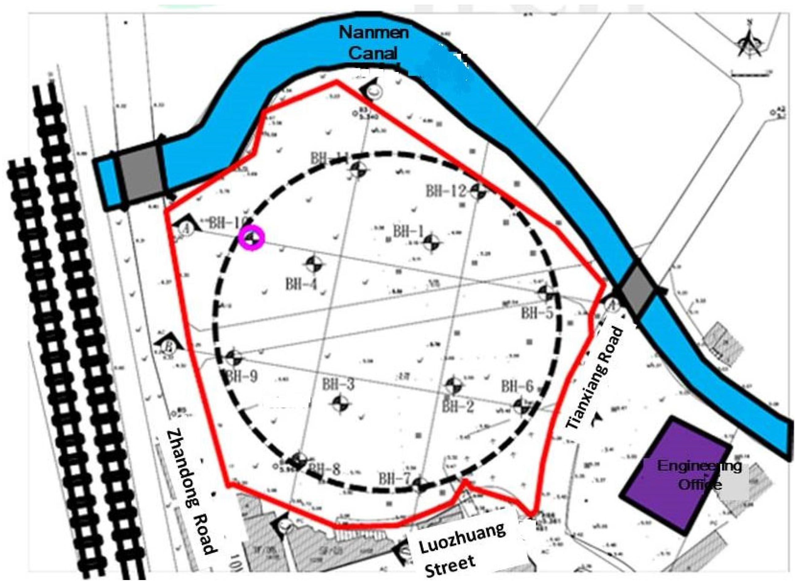
This case study’s site is located at a construction site in Luodong Town, Yilan County. The project involves the construction of a new hotel with four underground levels and twenty-three above-ground levels. The site covers an area of approximately 10,008 square meters and has an irregular shape, although the terrain within the site is flat. To the north of the site, there is an open space and a river, while the south side is adjacent to a neighboring building with 3–5 floors above ground and an open space. On the east side, it is near an 8 m wide Heaven Road, and on the west side, it is close to a 10 m wide Station East Road, with a railway passing further to the west, as shown in Figure 2.
This study adopts a circular diaphragm wall with a diameter of 93.5 m (radius R = 46.75 m) as a soil retention measure (divided into 60 units, with unit lengths of approximately 4.8~4.9 m) and an excavation depth of 17.05 m. Considering the diaphragm wall’s body forms a closed and complete circle, it can effectively transform bending moments into axial compressive forces, eliminating the need for an internal support system and mid-columns. Therefore, during excavation operations, it significantly reduces construction difficulty, effectively accelerates project timelines, and minimizes the risks associated with the removal of the support system.
- (1)
- Soil Layer Overview
The site underwent geological drilling and sampling with a total of twelve holes, designated as BH-1 to BH-12. Among these, the depths of BH-1 and BH-3 are 70 m, BH-2 and BH-4 are 60 m, and BH-5 to BH-12 are 40 m. The locations of the drilling holes are shown in Figure 2, Drilling Location Map. The surface soil layer was drilled using a wash boring method combined with a fishtail drill bit. A standard penetration test (SPT) was conducted every 1.5 m or when there was a change in soil layers, and 2” ψ split-spoon samples were collected for general physical property tests. At appropriate depths within the surface layer, undisturbed 3” ψ thin-wall tube samples were collected for mechanical property testing; when encountering gravel layers, rotary drilling was employed. After compiling and analyzing drilling data from the twelve holes and based on the results of the laboratory tests on the general physical properties of the soil, it can be summarized that the strata within the investigated depth of the site can be generally divided into eleven layers.
- (2)
- Groundwater Level
At the site, 12 m deep water level observation wells were installed in holes BH-6, BH-9, and BH-12. Measurements taken during the survey period indicated that the groundwater level was approximately between GL −1.6 to −2.4 m. Additionally, piezometers were installed in the sandy soil layers at depths of approximately 57 m, 55.6 m, and 31 m in holes BH-2, BH-4, and BH-8, respectively. Measurements from these piezometers showed that the groundwater pressure head in these locations was approximately GL −1.3 to −1.9 m.
- (3)
- Construction Process of the Case
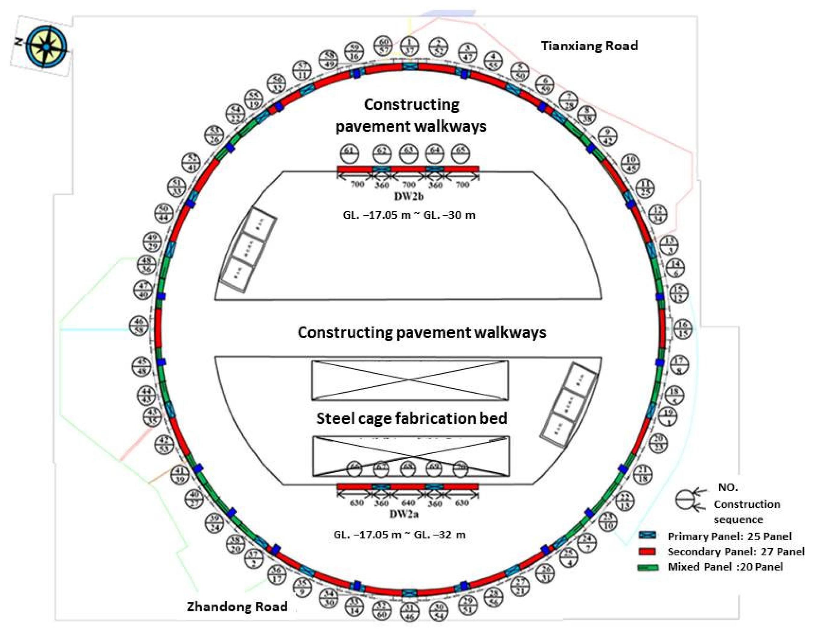
In this case, a circular diaphragm wall with a diameter of 93.5 m (radius R = 46.75 m) was used as a soil retention measure (divided into 60 units, with unit lengths approximately 4.8~4.9 m), with a wall thickness of 1 m and an excavation depth of 17.05 m. The construction process is as follows:
- A.
- Guide Trench for the Diaphragm Wall: An excavator digs to a depth of 3 m, then steel is tied inside, followed by the erection of formwork on the inside of the steel. Finally, concrete is poured outside the formwork to complete the guide trench.
- B.
- Before starting the excavation, dewatering wells are installed around the site to lower the groundwater from GL −1 m to GL −4.7 m. Pumping out water continues until the structure’s weight surpasses the groundwater’s buoyant force, allowing for the sealing of wells. This ensures a stable excavation and a dry work area for construction.
- C.
- Before constructing the roadway, an excavation 8 m wide and 25 cm deep is made. After pouring concrete, the roadway is completed (purpose: to prevent large vehicles from passing and compressing the diaphragm wall).
- D.
- After excavating the diaphragm wall trench to GL −36 m, the steel cage is lowered into the specified position, followed by concrete pouring and backfilling, and the diaphragm wall unit number and construction sequence are indicated in Figure 3.Figure 3. Diaphragm Wall Panel Numbering and Construction Sequence.
![Symmetry 16 00524 g003]()
- E.
- Antiflotation piles are constructed inside the site with the purpose of using the friction between the pile or diaphragm wall body (or cross wall, etc.) and the soil beneath to resist the upward force below the raft foundation slab, as shown in Figure 4.Figure 4. Anti-Flotation Pile (or Wall) Schematic Diagram.
![Symmetry 16 00524 g004]()
- F.
- For the excavation of the first underground layer, excavation proceeds from the inside out in a symmetrical manner, with each layer being 5 m deep to minimize displacement of the diaphragm wall. After the excavation inside the site is completed, the outer construction pavement is broken by an excavator, and excavation continues simultaneously.
- G.
- Excavation continues to the B1F level, and a ring beam is constructed. After exposing the reserved steel bars, the rebar is tied, the formwork is set up, and concrete is poured.
- H.
- The excavation of the second and third underground levels begins (during the curing period of the ring beam, starting with the middle excavation), and after 7 days of ring beam curing, it is excavated from below the ring beam.
- I.
- When excavating to the B3F level, a ring beam is constructed. After exposing the reserved steel bars, the rebar is tied, the formwork is set up, and excavation continues.
- J.
- Excavate the fourth and fifth underground levels (during the ring beam curing period, start with the middle excavation), and after 7 days of ring beam curing, excavate from below the ring beam.
- K.
- As the weight of soil in the excavation area continues to decrease and the amount of soapstone used to seal the drilling hole (BH-10) is insufficient, groundwater continuously flows out from the drilling hole, as shown in Figure 5 and Figure 6.Figure 5. Groundwater Continuously Flows Out from the Drilling Hole (Indicated by the Pink Circle and here, “BH-XX” in the figure refers to the XX drilling hole).Figure 5. Groundwater Continuously Flows Out from the Drilling Hole (Indicated by the Pink Circle and here, “BH-XX” in the figure refers to the XX drilling hole).
![Symmetry 16 00524 g005]() Figure 6. Groundwater Continuously Flows Out from the Drilling Hole (On-Site Situation).
Figure 6. Groundwater Continuously Flows Out from the Drilling Hole (On-Site Situation).![Symmetry 16 00524 g006]()
- L.
- Water is added to the excavation area until it reaches the same hydrostatic pressure as the groundwater outside the excavation area (at GL −6 m), as shown in Figure 7.Figure 7. Water Added to the Excavation Area Until It Matches the Hydrostatic Pressure of the Groundwater Outside the Excavation Area (The Green Circle Indicates the On-Site Situation).Figure 7. Water Added to the Excavation Area Until It Matches the Hydrostatic Pressure of the Groundwater Outside the Excavation Area (The Green Circle Indicates the On-Site Situation).
![Symmetry 16 00524 g007]()
- M.
- Before the CCP (Compacted Concrete Piling) grouting operation, a platform is set up, and the grouting machine is placed on the platform. After drilling around the drilling hole (down to GL −40 m), CCP grouting is performed from the outside to seal the inflow holes.
- N.
- After completing the CCP grouting, water inside the excavation area is pumped out.
- O.
- After lowering the groundwater outside the excavation area to GL −6 m and inside the excavation area to GL −18 m, excavation of the fourth and fifth underground levels continues.
- P.
- Before constructing the base of the fifth underground level, a layer of PC (Precast Concrete) with a thickness of 10 cm is laid.


- (4)
- Introduction to Monitoring Instruments
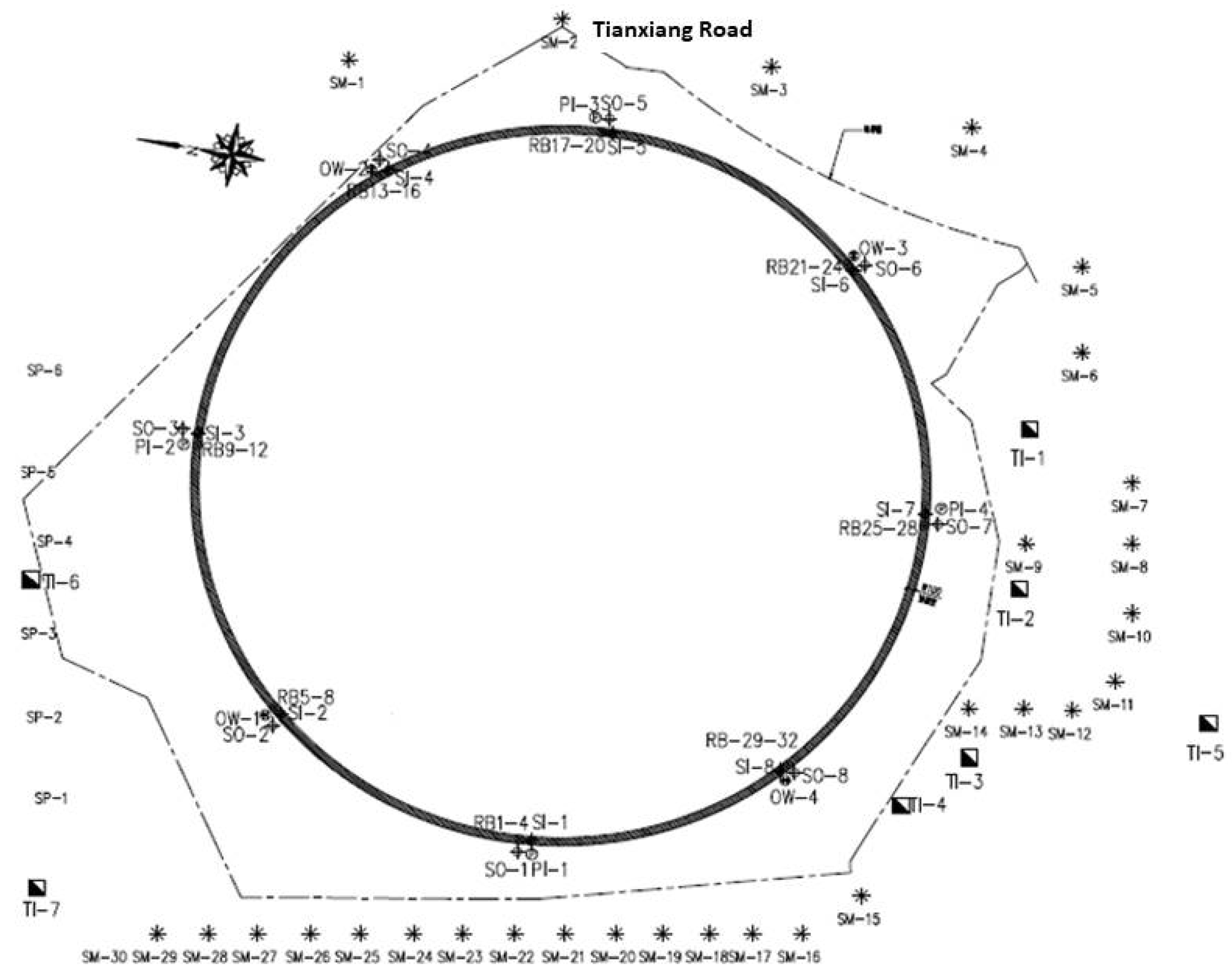
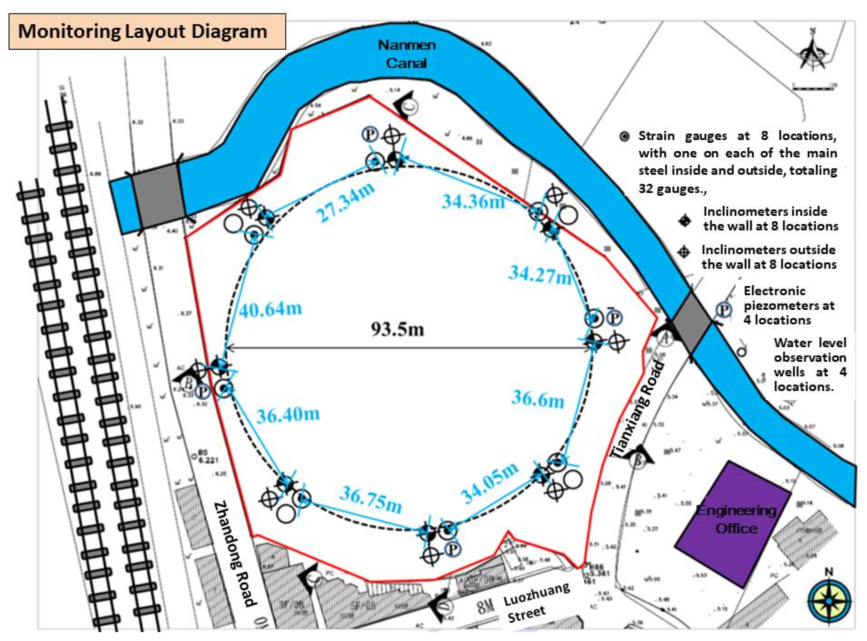
The safety monitoring items in this case include inclinometers inside and outside the diaphragm wall, strain gauges, water level observation wells, building inclinometers, settlement observation points, and electronic piezometers, as referenced in Appendix A Table A1 and Figure 8. To measure the displacement of the diaphragm wall, a total of 8 inclinometers were installed, reaching a depth of GL −36 m (the same depth as the diaphragm wall). To verify the accuracy of numerical model simulations, monitoring data from six inclinometers within the wall, SI-1, 3, 4, 5, 7, and 8, were compared with the results of numerical simulations. (SI-1 to SI-8 in Figure 9).
3. Numerical Simulation and Monitoring Data Validation
This study utilizes the numerical software PLAXIS 3D 2017 to simulate the deep excavation of a building site. Initially, it is necessary to document the surrounding conditions of the case site, the distribution of geological strata, the engineering properties of each stratum, the construction steps, and monitoring data. Then, using PLAXIS 3D, the complete excavation process is simulated. The content includes simulating the case results before and after water gushing occurrence using different models (MC, HS, and HSS) in PLAXIS 3D to compare with on-site monitoring data. This comparison verifies the accuracy of the modeling and the related parameter settings. Feedback analysis is employed to understand the changes in soil conditions at this time.
3.1. Numerical Simulation Model and Input Parameters
This case study focuses on the Luodong Hotel in Taiwan, which features an underground diaphragm wall set in a closed, symmetrical circular arrangement. Therefore, a full-circle model is adopted for simulation. According to a study by Ou and Shiau [22] and others, for the analysis of wall deformation, rollers should be placed at a distance of at least 3 to 5 times the excavation depth from the diaphragm wall. In this case study, the boundary is set to 5 times the excavation depth, with a soil layer setup depth of 71.6 m. The numerical model established is shown in Figure 10 and Figure 11. Additionally, the soil layer parameters are simplified into eleven layers, as detailed in Table 2.
- (1)
- Soil Layer Parameter Settings
For this case, the soil material composition law adopts the MC Model, HS model, and HSS model. By referencing empirical formulas from relevant scholars, assumptions, and calculations for parameters were made, summarized in Table 3 and Table 4:
- (2)
- Simulation of Circular Diaphragm Wall Parameters
In this case, the diaphragm wall thickness is 1.0 m, with the circular diaphragm wall construction depth ranging from GL + 0 to −36 m. The Young’s modulus of the diaphragm wall is derived from the Young’s moduli of concrete (Ec) and steel reinforcement (Es). Since the concrete section occupies a much larger proportion than the reinforcement section, the diaphragm wall’s Young’s modulus is represented by that of concrete. According to ACI standards, the concrete Young’s modulus is Ec = 15,000 × √fc’ (kgf/cm2), where fc’ is the compressive strength of concrete at 28 days. For this case study, fc’ is taken as 245 kgf/cm2 from the simplified soil layer parameter table, resulting in Ec = 23,032,618 kN/m2. This study utilizes Plaxis’s built-in plate elements to simulate the circular diaphragm wall and anti-flotation piles, with the latter extending from the ground surface (GL.0m) to the excavation depth of the site (GL −17.05 m). Due to incomplete actual data collection, the simulation uses the original soil layer parameters, detailed in Table 5. Furthermore, the typical Poisson’s ratio (ν) for concrete ranges between 0.1 and 0.2; thus, in the concrete simulation, ν is taken as 0.15. Additionally, Plaxis’s built-in beam elements are used to simulate ring beams, with the material’s Young’s modulus the same as that of diaphragm wall concrete, detailed in Table 6.
3.2. Simulation of Construction Steps
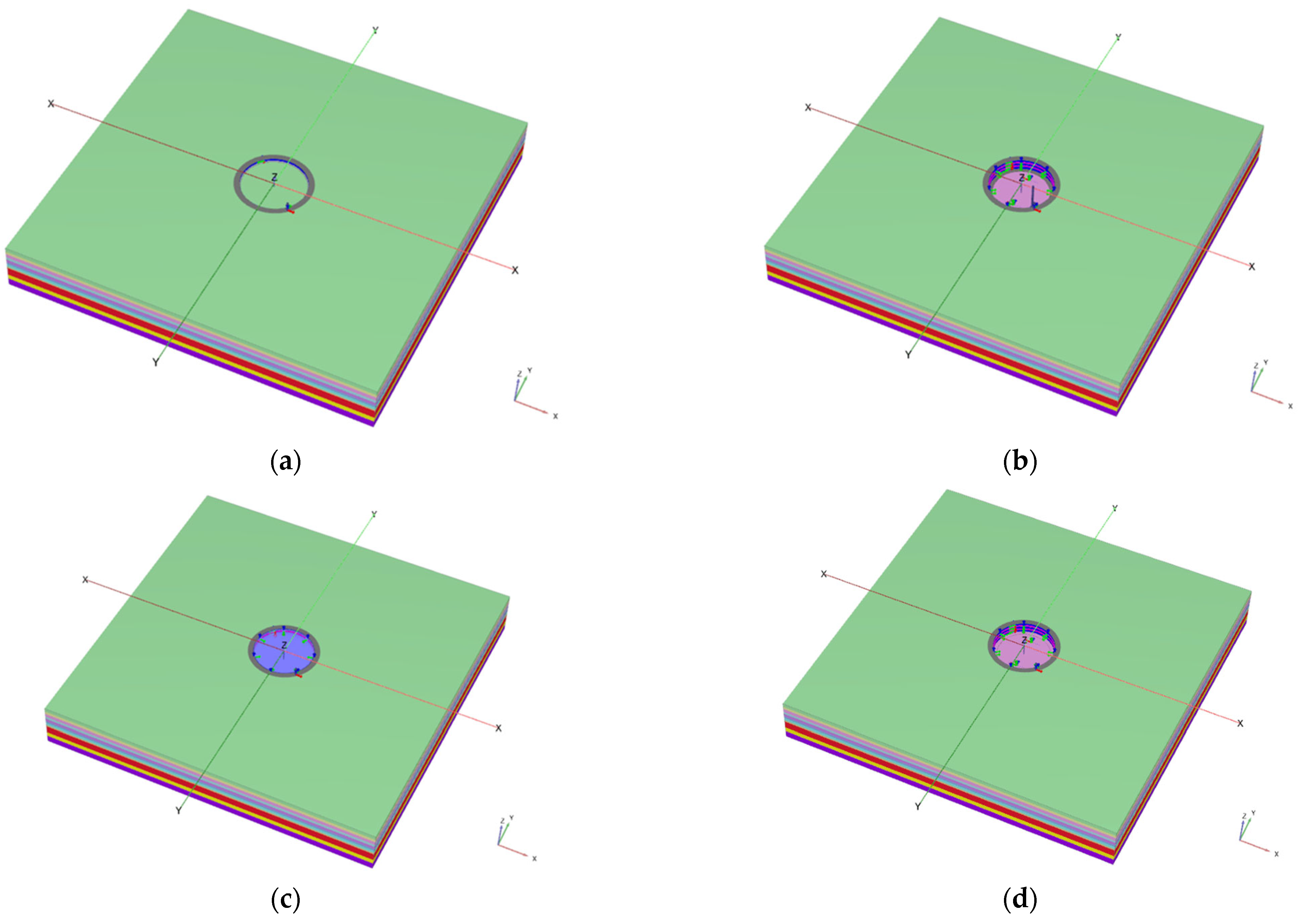
As mentioned in Section 2, when excavating to the fifth underground level (about to reach the bottom, GL −17.05 m), well No. 10 experienced water gushing due to the removal of the upper soil layers and insufficient bentonite used during the sealing of the drilling hole, leading to water gushing. Therefore, this study adds the simulation of water gushing within the excavation area. Before the occurrence of water gushing, the central area within the excavation zone had been dug to the bottom, with only piles of soil on both sides yet to be removed, as shown in Figure 12a. In the simulation, a simplified approach is adopted by converting the weight of the soil piles into surface loads applied on the final excavation surface (GL −17.05 m) to simulate, which is defined as the normal excavation simulation in this study, as shown in Figure 12b. Thus, site monitoring data of the piles of soil not yet excavated are used to verify whether the results of the simplified simulation are reasonable.
Using PLAXIS 3D 2017 software to analyze and simulate construction steps, this study is divided into two types of excavation construction modes. The first mode simulates normal excavation construction (simulating situations without water gushing inside the excavation area), consisting of 6 construction stages. The second mode simulates water gushing within the excavation area, consisting of 8 construction stages. Based on these simulations, the effects of the excavation process on the deformation of the retaining wall and the settlement of the surrounding strata are explored. The results are then compared with on-site observation data to verify the accuracy of the modeling approach and related parameters used in this research.
- Simulation of normal excavation construction steps (without water gushing inside the excavation area):
- (1)
- Set up the diaphragm wall, anti-flotation pile walls, and roadway (with a load of 33.75 kN/m2), and calculate the initial Ko stress before excavation.
- (2)
- Perform the first excavation (GL −5 m) calculation, lower the groundwater level to (GL −6 m) while the groundwater level outside the excavation area remains unchanged (GL −1 m), as detailed in Figure 13a.
- (3)
- Install the first layer of ring beam support (GL −4.75 m), with the groundwater level outside the excavation area remaining unchanged (−1 m).
- (4)
- Perform the second excavation (GL −12 m) and lower the groundwater level to (GL −13 m), while the groundwater level outside the excavation area remains unchanged (GL −1 m).
- (5)
- Install the second layer of ring beam support (GL −11.55 m), with the groundwater level outside the excavation area remaining unchanged (GL −1 m).
- (6)
- Perform the third excavation (GL −17.05 m), apply surface load calculations, and lower the groundwater level to (GL −18.05 m), while the groundwater level outside the excavation area remains unchanged (GL −1 m), as detailed in Figure 13b.
- Simulation of water gushing within the excavation area:The first six steps are the same as above.
- (7)
- Simulate water gushing within the excavation area up to GL −6 m while the groundwater level outside the excavation area remains unchanged (GL −1 m), as detailed in Figure 13c.
- (8)
- Pump out the water gushing inside the excavation area, and lower the groundwater level to (GL −18.05 m), then perform the final excavation to the bottom (GL −17.05 m) calculation, as detailed in Figure 13d.
3.3. Comparison of Simulation and On-Site Monitoring
This section will compare and analyze the results of the two excavation construction modes described in Section 3.2 with on-site monitoring data.
- Comparison of simulated normal excavation construction steps with on-site monitoring:
- (1)
- Comparison of simulation results with inclinometer data from on-site monitoring
According to the results simulated with the same soil parameters “clay = 800 Su, and = 2500 N” under three models, MC, HS, and HSS, the HS and HSS models produced similar outcomes. At the second excavation level (GL −12 M), the deformation in the HS model was greater than in the HSS model. Additionally, the MC model showed increasing deformation beyond a depth of 30 m, which did not converge effectively, contrary to the general expectation that deformation below the final excavation surface (GL −17.05 m) would gradually decrease, as shown in Figure 14a.
Furthermore, the simulation results showed a displacement of 2.51 mm at the bottom of the diaphragm wall, similar to the displacement found in the simulation results by Yasushi and Osamu [3], indicating a higher credibility of this study’s simulation results. The normalized ratio of the horizontal displacement at the bottom of the diaphragm wall (2.51 mm) to the diameter of the circular diaphragm wall (93 m) is 0.00003, which is smaller than the range of 0.00009~0.00012 found in a study by Yasushi and Osamu [3], attributable to differences in the simulation of the diaphragm wall and excavation method. The comparison of the HS model with inclinometer data from on-site monitoring shows a discrepancy in the amount of deformation of the wall surface, with the deformation only exceeding the monitored values after the first ring beam (GL −4.75 m). The simulation predicted the maximum deformation at a depth of 12.0 m to be 12.9 mm, while the actual monitored maximum deformation was at a depth of 11.5 m with 11.6 mm. Although the simulated deformation exceeded the monitored values, the overall trend of the wall deformation simulated effectively represents the maximum deformation and its location as observed on-site, as shown in Figure 14b and Figure 15.
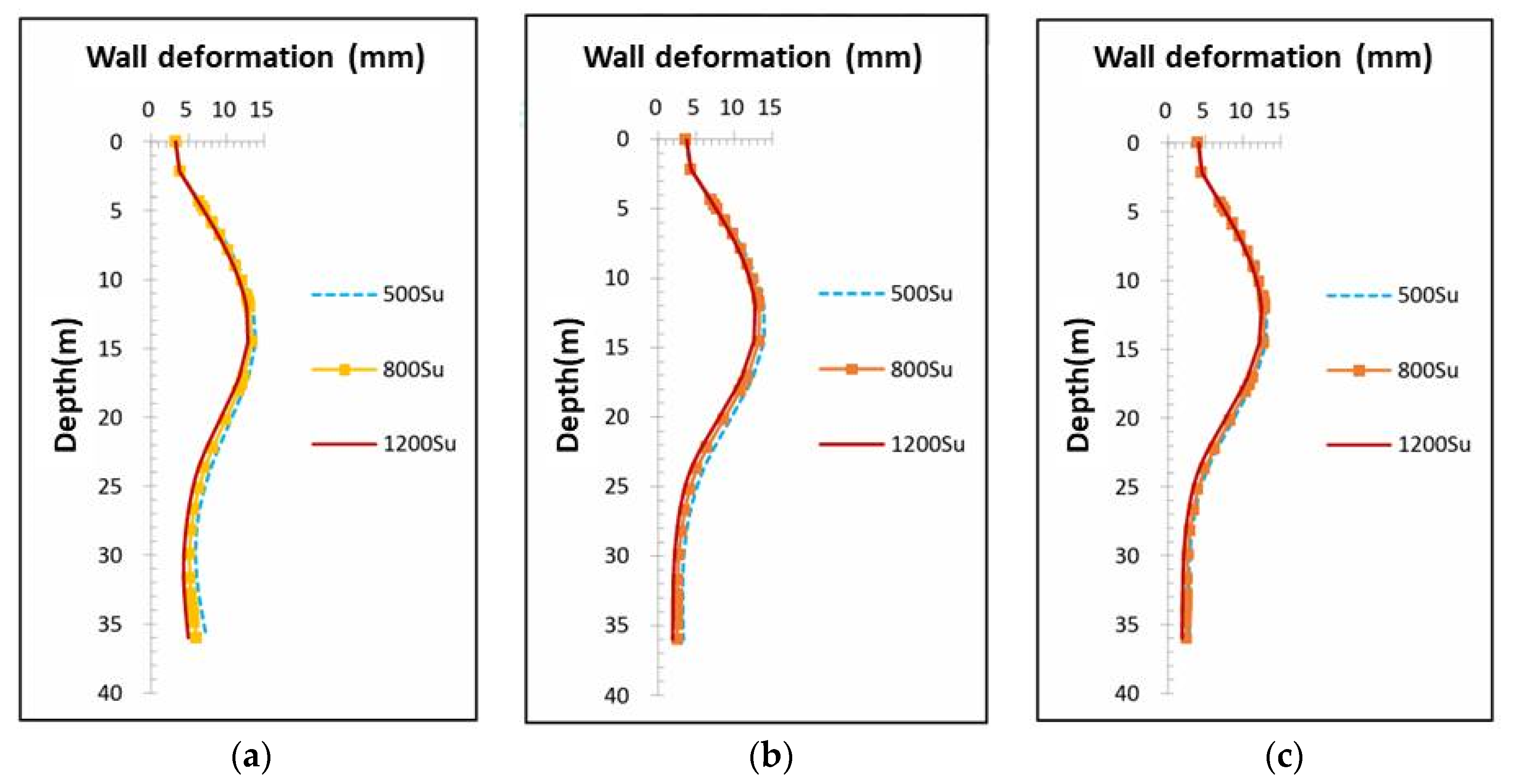
By simulating with the MC, HS, and HSS models, keeping the Young’s modulus of sand (2500 N) constant and changing the Young’s modulus of clay to “500 Su, 800 Su, 1200 Su”, the results showed that the parameters for 800 Su were between those for 500 Su and 1200 Su, as shown in Figure 16. According to the simulations with the MC, HS, and HSS models with the Young’s modulus of clay “500 Su, 800 Su, 1200 Su” Inclinometer SI-5 is the explanation.unchanged and changing the Young’s modulus of sand to “2000 N, 2100 N, 2200 N, 2300 N, 2400 N, 2500 N, 2600 N”, the results indicate that changing the N value has a limited impact on the deformation of the wall. The outcomes of the three models (MC, HS, and HSS) were almost identical. This result may be due to the characteristics of the circular diaphragm wall, as detailed in the Supplementary Material Figures S1–S3.
- (2)
- Comparison of ground settlement simulation results with on-site ground settlement data (SM2)
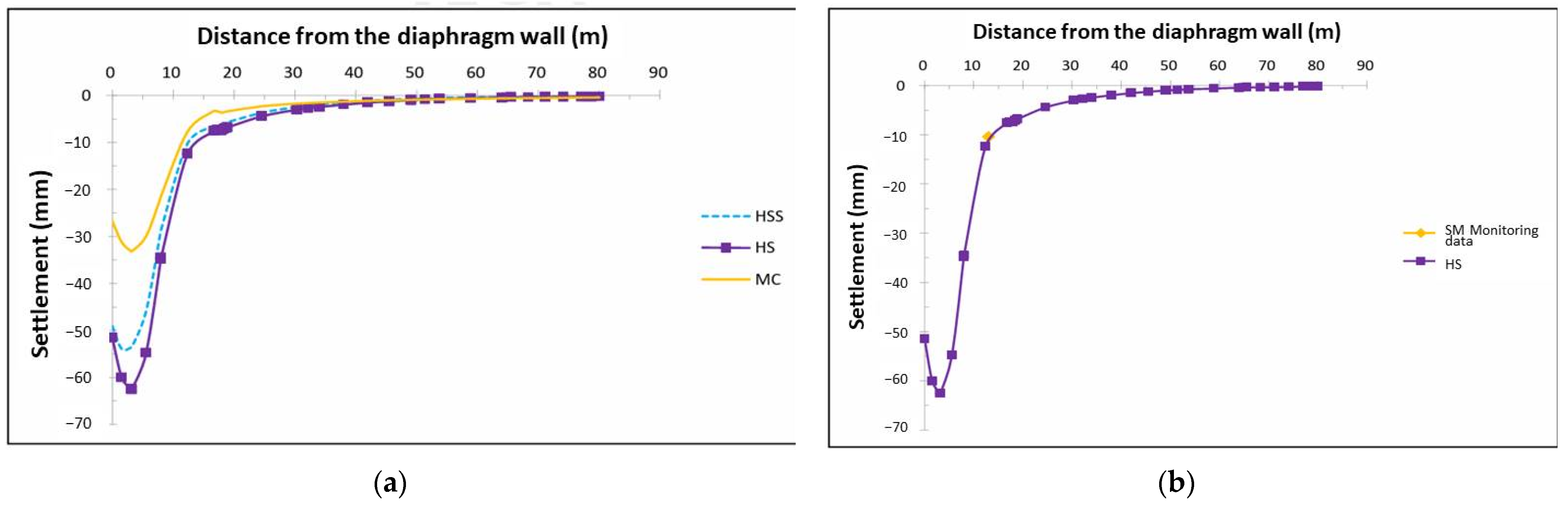
The relationship between the direction and distance of the circular diaphragm wall model and the ground settlement point (SM2) is shown in Figure 17. Based on the MC, HS, and HSS models using the same soil parameters “clay = 800 Su, sand = 2500 N” and sampling at 0.05 m below the ground surface, the results of ground settlement simulations show that the ground settlement is greater within 0 m to 8 m from the retaining wall, where the roadway is located, due to the weight and load of the roadway, as shown in Figure 18a. Within 40 m from the retaining wall, the ground settlement measured by the MC and HSS models is less than that by the HS model. Beyond 40 m, the settlement amounts of all three models have stabilized and are less than 1 mm. This is consistent with Peck’s [18] suggestion that the impact distance of ground settlement is four times the excavation depth (GL −17.05 m) and also aligns with Clough and O’Rourke’s [10] suggestion that the impact range of ground settlement is 2 to 3 times the excavation depth (GL −17.05 m). The comparison of ground settlement amounts from the HS model with on-site monitoring data at point (SM2) shows that the simulation results are very close to the actual ground settlement. This suggests that although the ground settlement amount from the HS model is greater than those from the MC and HSS models, it can effectively predict the amount of ground settlement at the end of normal excavation, as shown in Figure 18b.
With the Young’s modulus of sand (2500 N) unchanged and varying the Young’s modulus of clay to “500 Su, 800 Su, 1200 Su”, the results for 800 Su parameters were found to be between those for 500 Su and 1200 Su, as shown in Figure 19. According to the MC, HS, and HSS models with the Young’s modulus of clay “500 Su, 800 Su, 1200 Su” constant and changing the Young’s modulus of sand to “2000 N, 2100 N, 2200 N, 2300 N, 2400 N, 2500 N, 2600 N”, the results indicate that changing the N value has limited impact on ground settlement amounts. There is a noticeable difference in ground settlement within 5 m to 8 m from the retaining wall due to the influence of the roadway. Beyond 8 m from the retaining wall, the simulation results of the MC, HS, and HSS models are almost identical, as detailed in Supplementary Material Figures S4–S6.
- (3)
- Comparison of ground settlement simulation results with on-site ground settlement data (SM16~30)
Information on the distance of ground settlement points SM16~30 from inclinometer SI-1 is depicted in Figure 20. The simulation results from the MC, HS, and HSS models, using the same soil parameters “clay = 800 Su, sand = 2500 N” and sampling at 0.05 m below the ground surface, indicated that the deformation increases as the settlement points are closer to the circular diaphragm wall, aligning with the findings from previous studies. Furthermore, the analysis results of the three models show the same trend as data for settlement point SM2, where the amount of ground settlement in the HS model is greater than that in the MC and HSS models, as shown in Figure 21a. The comparison of ground settlement amounts from the HS model with on-site monitoring data reveals that only the analysis data for settlement points SM17 and SM19 are close to the actual monitoring values, whereas analysis data for the remaining points significantly differ from the on-site monitoring values, as shown in Figure 21b. This discrepancy is hypothesized to result from the settlement points being located on the access routes of construction vehicles, causing distortion in the settlement measurements at these points.
- Comparison of simulated water gushing within the excavation area with on-site monitoring
This study utilizes the Mohr–Coulomb model (MC), the Hardening Soil model (HS), and the Hardening Soil Small Strain model (HSS) to simulate the situation after water gushing occurs within the excavation area. The primary Young’s moduli (E) used are “clay = 800 Su, sand = 2500 N”. The simulation results are then compared with on-site monitoring inclinometer data from SI1, 3, 4, 5, 7, and 8. The aim is to observe if the inclinometer shifts away from the excavation area during water pouring and pumping within the excavation area to see if the simulated water gushing aligns with the changes observed in on-site monitoring.
- (1)
- Comparison of water gushing simulation results with on-site monitoring inclinometer data
According to the MC, HS, and HSS models with the same soil parameters, “clay = 800 Su, sand = 2500 N”, the results of simulating water gushing followed by excavation to the bottom show that a noticeable difference in deformation only appears at the location of the second layer of ring beam (GL −11.55 m) across all three models. Furthermore, the wall deformation after excavation to the bottom in the MC, HS, and HSS models is slightly greater than that in normal excavation, as shown in Figure 22a and Figure 23c. The comparison between the wall deformation from water gushing and the on-site monitoring data does not match. This discrepancy is hypothesized to be due to the imbalance of soil water pressure inside and outside the excavation area when water gushing occurs, leading to uneven forces on the diaphragm wall and excessive deformation of the inclinometers. Even after resolving the water gushing and excavating to the bottom, the deformation of the wall has already been distorted, as shown in Figure 22a.
- (2)
- Comparison of wall deformation results between normal excavation simulation and water gushing simulation
4. Conclusions
4.1. Summary
From the above analysis results, the following conclusions can be drawn:
- Model Evaluation for Normal Excavation: This study utilizes three models to assess soil behavior. The HS model demonstrates higher accuracy in capturing soil deformations under normal excavation conditions. With parameters “clay = 800 Su, sand = 2500 N”, both the HS and HSS models predict similar diaphragm wall displacements, but the HS model predicts less ground settlement, indicating a closer resemblance to real-site conditions.
- Effect of Young’s Modulus on Soil Behavior: Adjusting the clay Young’s modulus at three different levels shows that 800 Su best represents real soil behavior. The modulus of sand has minimal impact on wall deformation and settlement, highlighting the limited effect of Young’s modulus in scenarios with mixed soil conditions.
- Accuracy of Ground Settlement Simulation: Under the parameters “clay = 800 Su, sand = 2500 N”, the HS model’s simulation of ground settlement aligns well with on-site data at site SM2, away from construction traffic. Conversely, sites SM16~30, located on traffic routes, recorded higher settlements than simulated, pointing to discrepancies likely influenced by external factors.
- Support from Previous Studies: The simulation results of horizontal displacement at the bottom of the diaphragm wall are corroborated by findings from Yasushi and Osamu [3], enhancing the credibility of these results.
- Water Gushing Simulations: Simulations of water gushing conditions revealed significant disparities with on-site data, suggesting the models’ limitations in accurately reflecting real-time soil and water pressure dynamics, which cause notable outward wall inclinations.
- Wall Deformation Under Normal Excavation: The HS model estimated a maximum wall deformation of 12.9 mm at a depth of 12.0 m, slightly higher than the observed 11.6 mm at 11.5 m depth. This discrepancy, along with variations in wall diameter, depth, and external loads compared with the existing literature (Peck [18]), underscores the need for further investigation.
- Ground Settlement Near Excavation Site: Using the HS model parameters for normal excavation up to GL −17.05 m, the simulation indicated a maximum ground settlement of 62.59 mm at 8 m from the diaphragm wall. This exceeded empirical expectations and was likely influenced by nearby roadway traffic and load effects on soil behavior.
This study utilizes numerical simulation techniques to assess the impact of the uncommon circular diaphragm wall under various soil conditions, particularly in scenarios involving water gushing. It not only provides a thorough analysis of the current models’ limitations in simulating dynamic soil-water pressure interactions but also clearly identifies the necessity for further improvements to these models. These analyses highlight the innovative nature and practical value of this research, demonstrating how accurate simulations can enhance the safety and efficiency of construction projects.
4.2. Recommendations
- Circular Diaphragm Wall Analysis: Using Plaxis 3D, this study found that the Hardening Soil model (HS) closely matched the actual maximum wall deformations for a circular diaphragm wall. Ground settlement at point SM2 was accurate, but discrepancies at points SM16~30 suggest the need for a specific arrangement of settlement monitoring points to avoid distortions from construction activities.
- Soil Behavior Analysis with Three Models: This study employed three models (MC, HS, HSS) using effective stress parameters due to the lack of comprehensive total stress data. This underscores the necessity for more detailed soil data to enhance simulation accuracy in future research.
- Use of Circular Diaphragm Wall: The application of a circular diaphragm wall with unsupported excavation is uncommon domestically. Additional successful case studies are essential for a better understanding of wall displacement and ground settlement, thus improving analysis references.
Supplementary Materials
The following supporting information can be downloaded at: https://www.mdpi.com/article/10.3390/sym16050524/s1, Figure S1; Figure S2; Figure S3; Figure S4; Figure S5; Figure S6.
Author Contributions
Conceptualization S.-L.C. and Y.-H.T.; methodology, Y.-H.T., C.-F.H. and S.-L.C.; formal analysis, Y.-H.T. and C.-F.H.; investigation, K.-H.H.; writing—original draft preparation, C.-F.H.; writing—review and editing, C.-F.H.; supervision S.-L.C. All authors have read and agreed to the published version of the manuscript.
Funding
This research received no external funding.
Data Availability Statement
The data are contained within the article and Supplementary Materials.
Conflicts of Interest
The authors declare no conflict of interest.
Appendix A

Table A1.
Explanation of the excavation safety monitoring system diagram and management values.
| Illustration | Description | Management Item | Measurement Frequency | Alert Value (cm) | Action Value (cm) | |
|---|---|---|---|---|---|---|
| 1 |  | Inclinometer observations inside the wall at 8 locations, required to be embedded at GL −36 m. | Lateral displacement of the retaining wall | During the excavation phase, observations are conducted twice a week, normally once a week. | 1.6 | 2.5 |
| 2 |  | Inclinometers in the soil at 8 locations, each location 5 m deeper than the diaphragm wall. | Lateral displacement of the soil layers | During the excavation phase, observations are conducted twice a week, normally once a week. | 1.6 | 2.5 |
| 3 |  | Strain gauges at 8 locations, each installed at depths of GL −11.8 m and GL −22.2 m on the main reinforcement bars inside and outside, with a total of 32 strain gauges installed. | Stress in the reinforcement of the diaphragm wall | During the excavation phase, observations are conducted daily at fixed times, normally once every two days. | 2100 Kgf/cm2 | 2520 Kgf/cm2 |
| 4 |  | Water level observation wells at 4 locations, each with a depth of 12 m. | Groundwater level around the site | Observations are conducted twice a week. | 2 m | 3 m |
| 5 |  | Building tilt meters at a minimum of 8 locations are to be installed near buildings and pedestrian bridges at the construction site (arranged by the contractor). | Tilt of neighboring buildings near the site | During the excavation phase, observations are conducted twice a week, normally once a week. | 1/500 | 1/300 |
| 6 |  | Additionally, at least 30 settlement observation points are to be set up on roads, buildings, and pedestrian bridges surrounding the construction site (arranged by the contractor). | Ground settlement near the site (cm) | During the excavation phase, observations are conducted twice a week, normally once a week. | 1.6 | 2.5 |
| 7 |  | Electronic water pressure gauges at 4 locations, positioned 39 m below the ground surface. | Groundwater pressure within the site and beneath the excavation face | During the excavation phase, observations are conducted daily at fixed times, normally once every two days. | See details below. | See details below. |
Remarks: For all safety monitoring facilities, the contractor should establish observation safety values and analysis methods and propose construction, monitoring feedback, and contingency plans. These must be approved by the urban management unit and structural engineers before implementation.
References
- Wen-Han, P. The Study of the Performances of a Large-Scale Cofferdam Excavation. In Institute of Civil Engineering & Disaster PreVention Technology; National Kaohsiung University of Applied Sciences: Kaohsiung, Taiwan, 2008. [Google Scholar]
- Kim, D.-S.; Lee, B.C. Cylindrical Diaphragm Wall Movement During Deep Excavation For In-ground LNG Storage Tankin Coastal Area. Int. J. Offshore Polar Eng. 2003, 13, 285. [Google Scholar]
- Arai, Y.; Kusakabe, O.; Murata, O.; Konishi, S. A numerical study on ground displacement and stress during and after the installation of deep circular diaphragm walls and soil excavation. Comput. Geotech. 2008, 35, 791–807. [Google Scholar] [CrossRef]
- Wang, W.; Zhu, W.; Chen, Z.; Weng, Q.; Wu, J. Design, study and practice of deep cylindrical excavation of Shanghai World Expo 500 kV underground transmission substation project. Chin. J. Geotech. Eng. 2008, 30, 564–576. [Google Scholar]
- Tan, Y.; Lu, Y.; Xu, C.; Wang, D. Investigation on performance of a large circular pit-in-pit excavation in clay-gravel-cobble mixed strata. Tunn. Undergr. Space Technol. 2018, 79, 356–374. [Google Scholar] [CrossRef]
- Xu, Q.W.; Xie, J.L.; Zhu, H.H.; Lu, L.H. Supporting behavior evolution of ultra-deep circular diaphragm walls during excavation: Monitoring and assessment methods comparison. Tunn. Undergr. Space Technol. 2024, 143, 105495. [Google Scholar] [CrossRef]
- Lim, A.; Ou, C.-Y. Case Record of a Strut-free Excavation with Buttress Walls in Soft Soil. In Proceedings of the 2nd International Symposium on Asia Urban GeoEngineering, Singapore, Changsha, China, 24–27 November 2018; pp. 142–154. [Google Scholar]
- Chuah, S.; Harry, S.T. Numerical study on a new strut-free counterfort embedded wall in Singapore. In Proceedings of the Earth Retention Conference 3, Washington, DC, USA, 1–4 August 2010. [Google Scholar]
- Chiu, H.-W.; Hsu, C.-F.; Tsai, F.-H.; Chen, S.-L. Influence of Different Construction Methods on Lateral Displacement of Diaphragm Walls in Large-Scale Unsupported Deep Excavation. Buildings 2024, 14, 23. [Google Scholar] [CrossRef]
- Clough, W.; O’Rourke, T. Construction induced movements of in situ wall. Geotech. Spec. Publ. 1990, 25, 439–470. [Google Scholar]
- Ou, C.-Y.; Hsieh, P.-G.; Chiou, D.-C. Characteristics of ground surface settlement during excavation. Can. Geotech. J. 1993, 30, 758–767. [Google Scholar] [CrossRef]
- Wang, J.-Z.; Chan, X.-S.; Lei, Y.-M. Analysis of Soil Parameters in the Kaohsiung Metro Red Line Section. J. Chin. Inst. Civ. Hydraul. Eng. 2003, 30, 101–104. [Google Scholar]
- Mana, A.I.; Clough, G.W. Prediction of movements for braced cuts in clay. J. Geotech. Eng. Div. 1981, 107, 759–777. [Google Scholar] [CrossRef]
- Masuda, T.; Einstein, H.H.; Mitachi, T. Prediction of lateral deflection of diaphragm wall in deep excavations. Doboku Gakkai Ronbunshu 1994, 1994, 19–29. [Google Scholar] [CrossRef] [PubMed]
- Hsiung, B.-C. Engineering Performance of Deep Excavations in Taipei. Ph.D. Thesis, University of Bristol, Bristol, UK, 2002. [Google Scholar]
- Hsu, C.-F.; Wu, C.-Y.; Li, Y.-F. Development of a Displacement Prediction System for Deep Excavation Using AI Technology. Symmetry 2023, 15, 2093. [Google Scholar] [CrossRef]
- Hsieh, P.-G.; Ou, C.-Y. Shape of ground surface settlement profiles caused by excavation. Can. Geotech. J. 1998, 35, 1004–1017. [Google Scholar] [CrossRef]
- Peck, B. Deep excavation and tunnelling in soft ground, State of the art volume. In Proceedings of the 7th International Conference on Soil Mechanics and Foundation Engineering (Mexico), Mexico City, Mexico, 25–29 August 1969; pp. 225–290. [Google Scholar]
- Woo, S.; Moh, Z. Geotechnical characteristics of soils in the Taipei basin. In Proceedings of the 10th Southeast Asian Geotechnical Conference, Taipei, Taiwan, 16–20 April 1990. [Google Scholar]
- Jia, J.; Zhai, J.Q.; Li, M.G.; Zhang, L.L.; Xie, X.L. Performance of Large-Diameter Circular Diaphragm Walls in a Deep Excavation: Case Study of Shanghai Tower. J. Aerosp. Eng. 2019, 32, 04019078. [Google Scholar] [CrossRef]
- Goh, A.T. Basal heave stability of supported circular excavations in clay. Tunn. Undergr. Space Technol. 2017, 61, 145–149. [Google Scholar] [CrossRef]
- Ou, C.-Y.; Shiau, B.-Y. Analysis of the corner effect on excavation behaviors. Can. Geotech. J. 1998, 35, 532–540. [Google Scholar] [CrossRef]
Figure 1.
Relationship between diaphragm wall thickness and deformation.
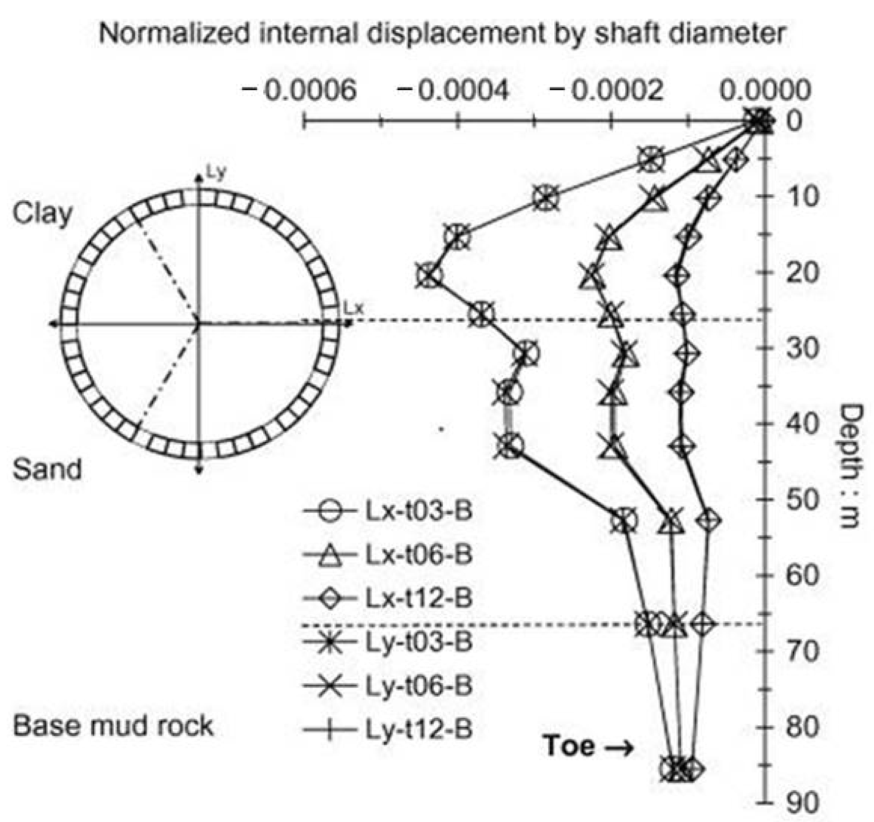
Figure 2.
Site Drilling Location Map.
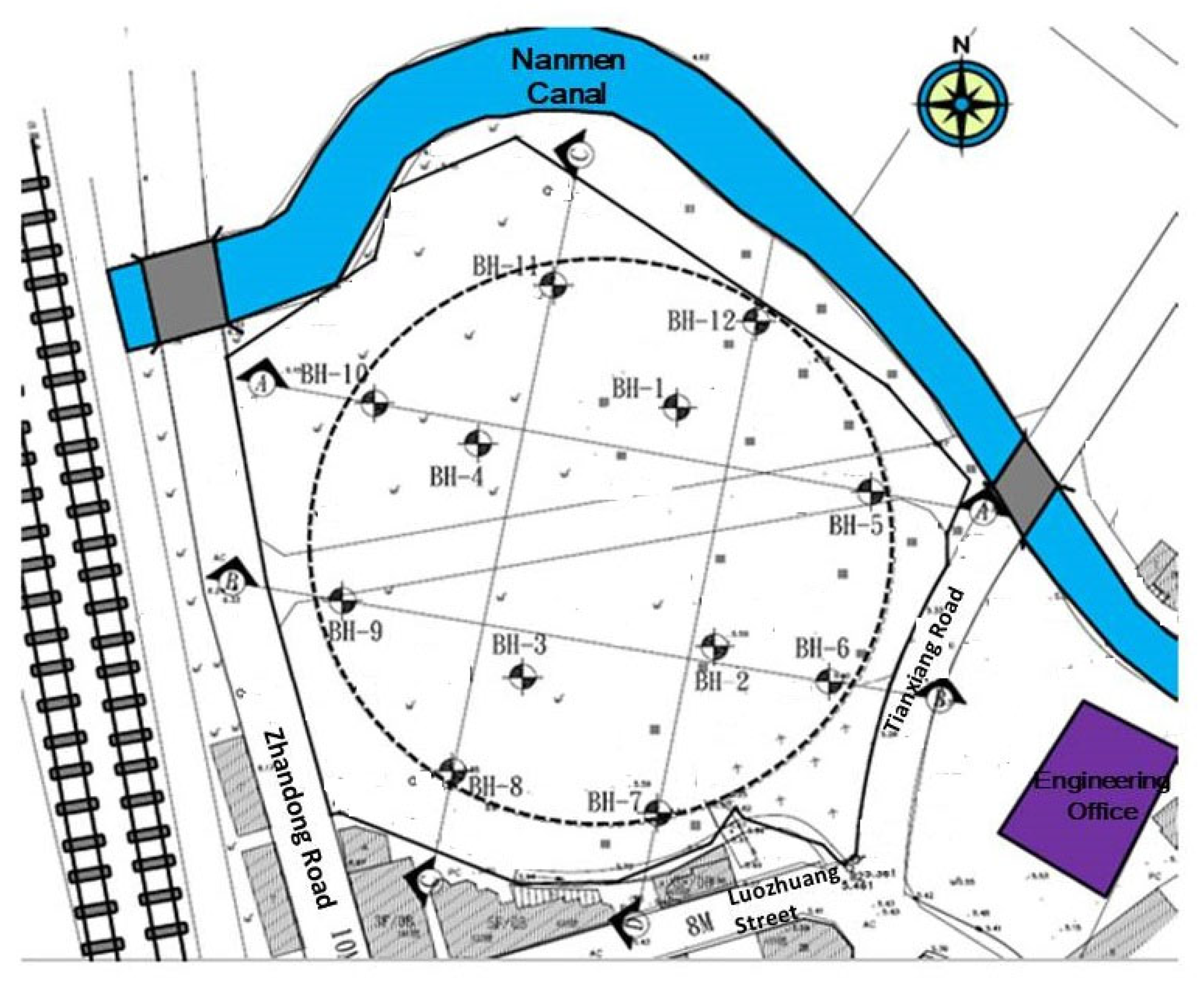
Figure 8.
Monitoring System Layout Diagram.

Figure 9.
Inclinometer Layout Diagram.

Figure 10.
(a) Schematic of the PLAXIS 3D numerical model for the circular diaphragm wall; (b) Top view; (c) Section view.
Figure 10.
(a) Schematic of the PLAXIS 3D numerical model for the circular diaphragm wall; (b) Top view; (c) Section view.

Figure 11.
Mesh diagram of the PLAXIS 3D numerical model for the circular diaphragm wall.

Figure 12.
The middle area inside the excavation zone has been excavated to the bottom, with piles of soil remaining on both sides. (a) Schematic diagram; (b) Simulation schematic diagram.
Figure 12.
The middle area inside the excavation zone has been excavated to the bottom, with piles of soil remaining on both sides. (a) Schematic diagram; (b) Simulation schematic diagram.

Figure 13.
Key Construction Step Comparison Chart (a) Step 2: First excavation (GL −5 m); (b) Step 6: Third excavation (GL −17.05 m); (c) Step 7: Simulate water gushing within the excavation area up to GL −6 m; (d) Step 8: Pump out the water gushing inside the excavation area.
Figure 13.
Key Construction Step Comparison Chart (a) Step 2: First excavation (GL −5 m); (b) Step 6: Third excavation (GL −17.05 m); (c) Step 7: Simulate water gushing within the excavation area up to GL −6 m; (d) Step 8: Pump out the water gushing inside the excavation area.

Figure 14.
Comparison of results from various soil models (800 Su, 2500 N) with monitoring data. (a) MC, HS, and HSS models; (b) HS model results compared with monitoring data.
Figure 14.
Comparison of results from various soil models (800 Su, 2500 N) with monitoring data. (a) MC, HS, and HSS models; (b) HS model results compared with monitoring data.

Figure 15.
Comparison of inclinometer SI-5 data with numerical analysis results (HS) at various excavation stages.
Figure 15.
Comparison of inclinometer SI-5 data with numerical analysis results (HS) at various excavation stages.
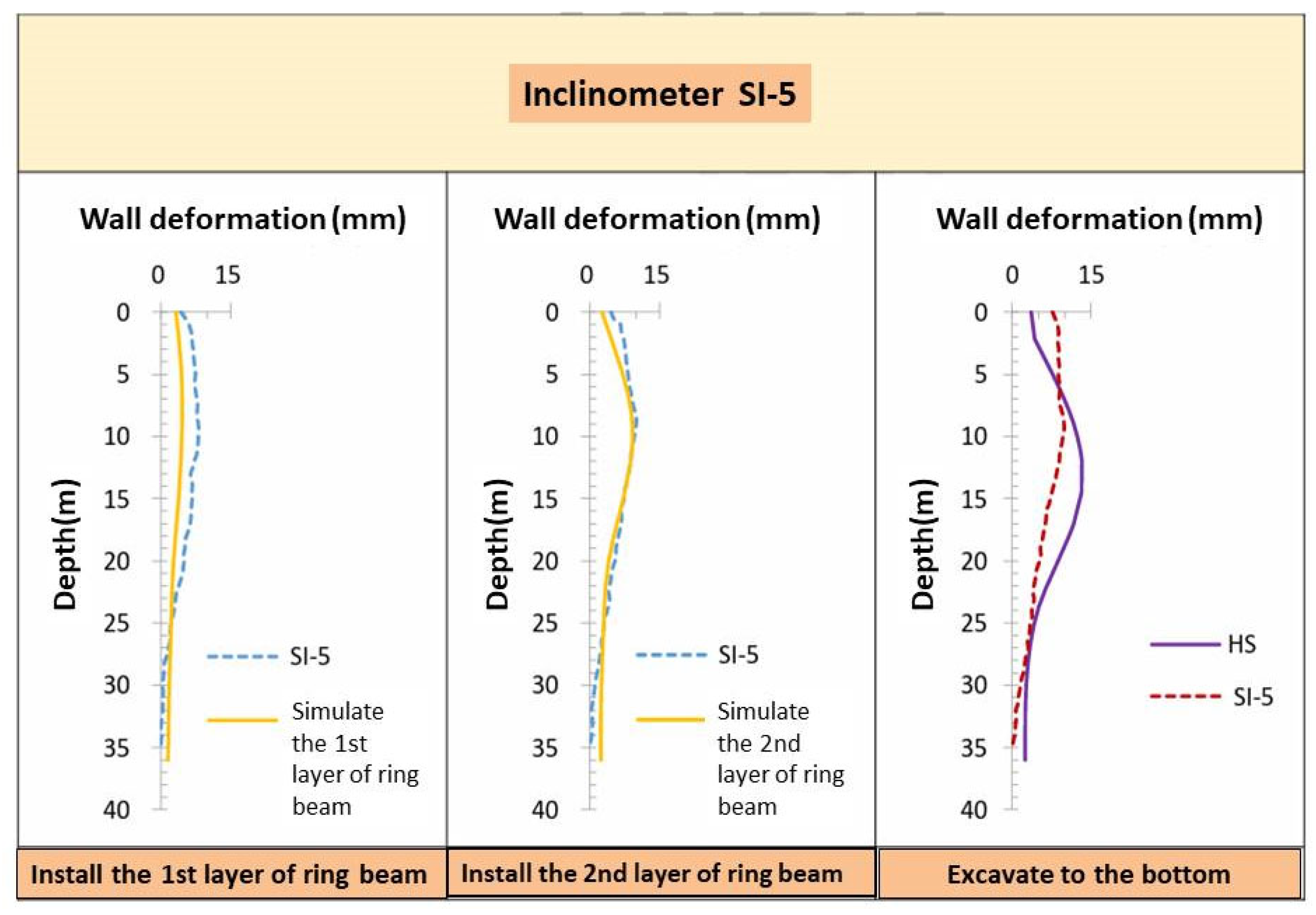
Figure 16.
Comparison of results with sand Young’s modulus (2500 N) held constant, and clay Young’s modulus varied. (a) MC Model; (b) HS Model; (c) HSS Model.
Figure 16.
Comparison of results with sand Young’s modulus (2500 N) held constant, and clay Young’s modulus varied. (a) MC Model; (b) HS Model; (c) HSS Model.

Figure 17.
Direction and distance of ground settlement (SM2) from the circular diaphragm wall model.
Figure 17.
Direction and distance of ground settlement (SM2) from the circular diaphragm wall model.

Figure 18.
Comparison of results from various soil models (800 Su, 2500 N) with monitoring data. (a) MC, HS, and HSS model; (b) HS model results compared with ground settlement data (SM2).
Figure 18.
Comparison of results from various soil models (800 Su, 2500 N) with monitoring data. (a) MC, HS, and HSS model; (b) HS model results compared with ground settlement data (SM2).

Figure 19.
Comparison chart of the results with sand Young’s modulus (2500 N) held constant, and clay Young’s modulus varied across different models. (a) MC Model; (b) HS Model; (c) HSS Model.
Figure 19.
Comparison chart of the results with sand Young’s modulus (2500 N) held constant, and clay Young’s modulus varied across different models. (a) MC Model; (b) HS Model; (c) HSS Model.

Figure 20.
Information on the distance of ground settlement points SM16~30 from inclinometer SI-1.

Figure 21.
Comparison of models (800 Su, 2500 N) with ground settlement data (SM1630). (a) MC model, HS model, and HSS model; (b) Comparison of HS model with ground settlement data (SM1630).
Figure 21.
Comparison of models (800 Su, 2500 N) with ground settlement data (SM1630). (a) MC model, HS model, and HSS model; (b) Comparison of HS model with ground settlement data (SM1630).

Figure 22.
Comparison of models (800 Su, 2500 N) for water gushing with ground settlement data (SM16~30). (a) MC, HS, and HSS models; (b) HS water gushing model and monitoring data.
Figure 22.
Comparison of models (800 Su, 2500 N) for water gushing with ground settlement data (SM16~30). (a) MC, HS, and HSS models; (b) HS water gushing model and monitoring data.

Figure 23.
Comparison of wall deformation amounts in normal excavation and water gushing across different models (800 Su, 2500 N). (a) MC model; (b) HS model; (c) HSS model.
Figure 23.
Comparison of wall deformation amounts in normal excavation and water gushing across different models (800 Su, 2500 N). (a) MC model; (b) HS model; (c) HSS model.
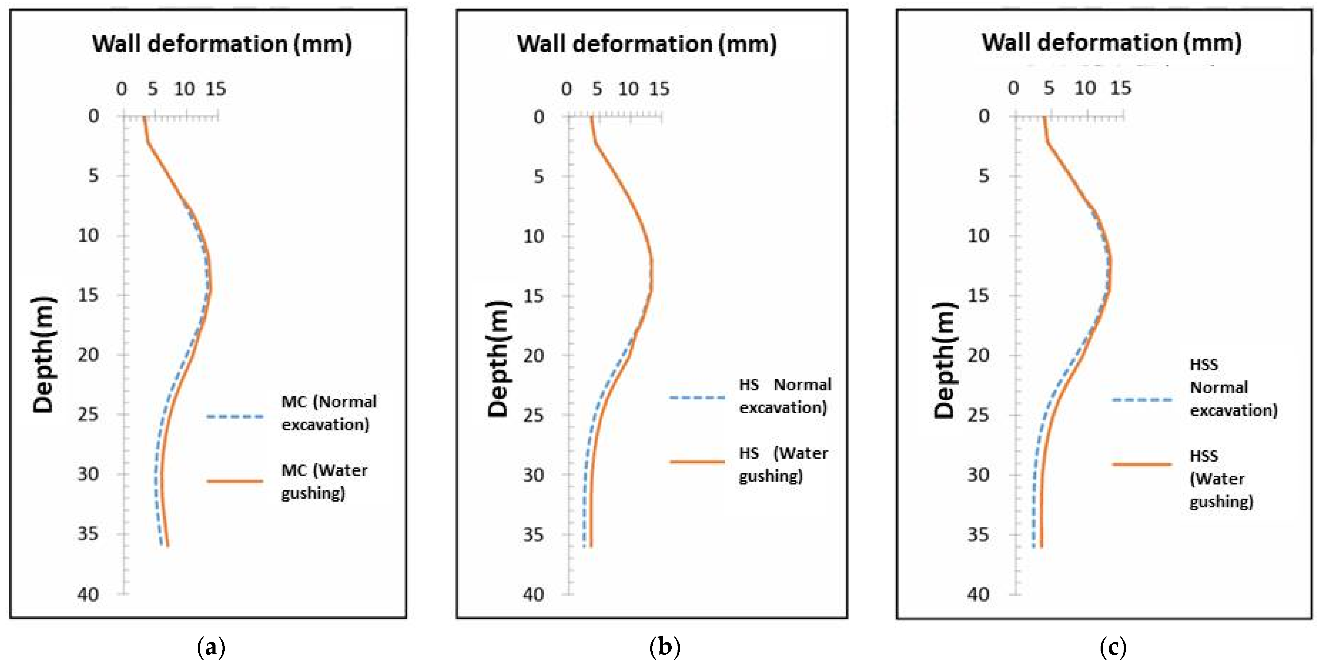
Table 1.
Results of Safety Factors and Various Parameters for Circular Diaphragm Wall Excavation.
| γ (KN/m3) | B (m) | T (m) | H (m) | D (m) | Co (kPa) | m | Ave Cu (kPa) | FSFE | FSshart |
|---|---|---|---|---|---|---|---|---|---|
| 16 | 40 | 60 | 16 | 4 | 5 | 1.5 | 39.5 | 1.288 | 1.287 |
| 16 | 40 | 60 | 16 | 4 | 10 | 1.5 | 44.5 | 1.473 | 1.450 |
| 16 | 40 | 60 | 16 | 4 | 20 | 1.5 | 54.5 | 1.813 | 1.776 |
| 16 | 40 | 60 | 16 | 10 | 10 | 1.5 | 53.5 | 1.923 | 1.952 |
| 16 | 40 | 72 | 24 | 4 | 10 | 1.5 | 56.5 | 1.285 | 1.291 |
| 16 | 40 | 80 | 24 | 12 | 10 | 1.5 | 68.5 | 1.748 | 1.785 |
| 16 | 100 | 120 | 24 | 24 | 10 | 1.5 | 93.25 | 2.192 | 2.180 |
| 16 | 20 | 60 | 16 | 10 | 10 | 1.5 | 51.25 | 2.177 | 2.300 |
| 16 | 20 | 60 | 16 | 4 | 10 | 1.5 | 42.25 | 1.544 | 1.610 |
| 16 | 30 | 60 | 16 | 4 | 10 | 1.5 | 43.375 | 1.479 | 1.498 |
| 16 | 40 | 60 | 16 | 4 | 20 | 1.2 | 47.6 | 1.584 | 1.551 |
| 16 | 40 | 60 | 16 | 4 | 10 | 1.2 | 37.6 | 1.246 | 1.225 |
| 16 | 40 | 60 | 16 | 10 | 10 | 1.2 | 44.8 | 1.617 | 1.634 |
Table 2.
Simplified Geotechnical Parameter Recommendation Table.
| Soil Layer | Average Depth (m) | γm (kN/m3) | N | Su (kN/m2) | CC | Cr | c (kN/m2) | Φ (°) | c’ (kN/m2) | φ’ (°) |
|---|---|---|---|---|---|---|---|---|---|---|
| ML/SM | 0~−6.88 ± 2.0 | 18.84 | 3 | 30 | − | − | 14.7 | 18 | * 0 | * 28 |
| CL/ML | −6.88~−11.7 ± 2.2 | 18.05 | 3 | 30 | − | − | 14.7 | 18 | * 0 | * 28 |
| ML/CL | −11.7~−18.1 ± 2.0 | 18.54 | 8 | 0.35 σ’ | * 0.2 | * 0.02 | 19.6 | 20 | 0 | 30 |
| SM | −18.1~−22.2 ± 1.1 | 19.03 | 12 | − | * 0.12 | * 0.012 | − | − | 0 | 31 |
| CL | −22.2~28.2 ± 1.5 | 18.54 | 9 | 0.35 σ’ | 0.21 | 0.033 | 19.6 | 20 | 0 | 30 |
| SM | −28.2~−31.7 ± 1.1 | 20.01 | 20 | − | * 0.10 | * 0.010 | − | − | 0 | 32 |
| CL, ML | −31.7~−36.7 ± 1.7 | 18.64 | 13 | 0.35 σ’ | 0.38 | * 0.039 | 19.6 | 21 | 4.9 | 30 |
| ML | −36.7~−39.1 ± 2.3 | 18.74 | 17 | − | * 0.12 | * 0.012 | − | − | * 0 | * 32 |
| ML, CL | −39.1~−52.4 ± 1.6 | 18.64 | 16 | 0.35 σ’ | 0.43 | 0.038 | 19.6 | 21 | 4.9 | 30 |
| SM | −52.4~−60.4 ± 0.5 | 20.11 | 35 | − | − | − | − | − | * 0 | * 35 |
| GM/SM | −60.4~−71.6 | 21.58 | 20 | − | − | − | − | − | * 0 | * 40 |
Note: 1. * indicates estimated values. 2. σ’ represents the effective overburden pressure, recommended based on the results of triaxial SUU tests. 3. Normal water level is recommended at GL −1 m; high water level is recommended at GL −0 m.
Table 3.
MC Model Soil Layer Parameter.
| Soil Layer | c’ (kN/m2) | φ’ (°) | ψ (°) | K0 | υ | Gs | ω (%) | e | K (cm/s) |
|---|---|---|---|---|---|---|---|---|---|
| 1. ML, SM | 0.2 | 28 | 0 | 0.53 | 0.30 | 2.7 | 23 | 0.62 | 3.25 × 10⁻⁴ |
| 2. CL, ML | 0 | 28 | 0 | 0.53 | 0.35 | 2.7 | 31 | 0.84 | 1.25 × 10⁻⁷ |
| 3. ML, CL | 0 | 30 | 0 | 0.50 | 0.35 | 2.7 | 31 | 0.84 | 1.25 × 10⁻⁷ |
| 4. SM | 0.2 | 31 | 1 | 0.48 | 0.30 | 2.7 | 29 | 0.78 | 3.25 × 10⁻⁴ |
| 5. CL | 0 | 30 | 0 | 0.50 | 0.35 | 2.7 | 29 | 0.78 | 1.25 × 10⁻⁷ |
| 6. SM | 0.2 | 32 | 2 | 0.47 | 0.30 | 2.7 | 21 | 0.57 | 3.25 × 10⁻⁴ |
| 7. CL, ML | 5 | 30 | 0 | 0.50 | 0.35 | 2.7 | 36 | 0.97 | 1.25 × 10⁻⁷ |
| 8. ML | 0.2 | 32 | 2 | 0.47 | 0.30 | 2.7 | 29 | 0.78 | 3.25 × 10⁻⁴ |
| 9. ML, CL | 5 | 30 | 0 | 0.50 | 0.35 | 2.7 | 31 | 0.84 | 1.25 × 10⁻⁷ |
| 10. SM | 0.2 | 34.5 | 4.5 | 0.43 | 0.30 | 2.7 | 20 | 0.54 | 3.25×10⁻⁴ |
| 11. GM, SM | 0.2 | 34.5 | 4.5 | 0.36 | 0.30 | 2.7 | 13 | 0.34 | 3.25×10⁻⁴ |
Table 4.
Soil Layer Parameter for the HS and HSS Models.
| Soil Layer | N | Su (kN/m2) | m | E50ref (kN/m2) | Eurref (kN/m2) | Eoedref (kN/m2) | e | Go (kN/m2) | G50ref (kN/m2) | γ0.7 |
|---|---|---|---|---|---|---|---|---|---|---|
| HS Model | Common Items | HSS Model | ||||||||
| 1. ML, SM | 3 | − | 0.5 | 7500 | 22,500 | 6000 | 0.62 | 61,566 | 112,330 | 6.88 × 10⁻⁵ |
| 2. CL, ML | 3 | 30 | 1.0 | 24,000 | 72,000 | 19,200 | 0.84 | 65,223 | 81,730 | 1.72 × 10⁻⁵ |
| 3. ML, CL | 8 | 44.41 | 1.0 | 35,532 | 106,596 | 28,425 | 0.84 | 103,681 | 81,730 | 1.77 × 10⁻⁵ |
| 4. SM | 12 | − | 0.5 | 30,000 | 90,000 | 24,000 | 0.78 | 116,334 | 88,523 | 2.16 × 10⁻⁵ |
| 5. CL | 9 | 75.88 | 1.0 | 60,704 | 182,112 | 48,563 | 0.78 | 191,954 | 88,523 | 1.63 × 10⁻⁵ |
| 6. SM | 20 | − | 0.5 | 50,000 | 150,000 | 40,000 | 0.57 | 196,076 | 121,605 | 1.95 × 10⁻⁵ |
| 7. CL, ML | 13 | 104.68 | 1.0 | 83,748 | 251,244 | 66,998 | 0.97 | 189,210 | 66,803 | 2.37 × 10⁻⁵ |
| 8. ML | 17 | − | 0.5 | 425,000 | 1,275,000 | 340,000 | 0.78 | 293,177 | 88,523 | 1.66 × 10⁻⁵ |
| 9. ML, CL | 16 | 139.68 | 1.0 | 111,748 | 335,244 | 89,398 | 0.84 | 306,719 | 81,730 | 1.93 × 10⁻⁵ |
| 10. SM | 35 | − | 0.5 | 87,500 | 262,500 | 70,000 | 0.54 | 282,090 | 126,533 | 2.61 × 10⁻⁵ |
| 11. GM, SM | 50 | − | 0.5 | 125,000 | 375,000 | 100,000 | 0.34 | 418,052 | 170,341 | 2.03 × 10⁻⁵ |
Table 5.
PLAXIS Plate Element Parameter.
| Type | Depth (m) | γ (kN/m3) | E (kN/m2) | Poisson’s Ratio υ | Thickness (m) |
|---|---|---|---|---|---|
| Diaphragm walls | GL + 0~−36 | 23.57 | 2.30 × 10⁷ | 0.15 | 1.0 |
| Anti-Flotation Pile | GL −17.05~−32 GL −17.05~−30 | 23.57 | 2.30 × 10⁷ | 0.15 | 1.0 |
Table 6.
PLAXIS Beam Element Parameter.
| Type | Area (m2) | γ (kN/m3) | E (kN/m2) | I1 | I2 |
|---|---|---|---|---|---|
| Ring Beam | 0.8 | 23.57 | 2.30 × 10⁷ | 0.04267 | 0.06667 |
Disclaimer/Publisher’s Note: The statements, opinions and data contained in all publications are solely those of the individual author(s) and contributor(s) and not of MDPI and/or the editor(s). MDPI and/or the editor(s) disclaim responsibility for any injury to people or property resulting from any ideas, methods, instructions or products referred to in the content. |
© 2024 by the authors. Licensee MDPI, Basel, Switzerland. This article is an open access article distributed under the terms and conditions of the Creative Commons Attribution (CC BY) license (https://creativecommons.org/licenses/by/4.0/).
Share and Cite
MDPI and ACS Style
Tsai, Y.-H.; Hsu, C.-F.; Ho, K.-H.; Chen, S.-L. Emergency Strategies for Gushing Water of Borehole and Numerical Simulation on Circular Diaphragm Wall Excavation with Ring-Beams. Symmetry 2024, 16, 524. https://doi.org/10.3390/sym16050524
AMA Style
Tsai Y-H, Hsu C-F, Ho K-H, Chen S-L. Emergency Strategies for Gushing Water of Borehole and Numerical Simulation on Circular Diaphragm Wall Excavation with Ring-Beams. Symmetry. 2024; 16(5):524. https://doi.org/10.3390/sym16050524
Chicago/Turabian StyleTsai, Yi-Hao, Chia-Feng Hsu, Kuo-Hsiang Ho, and Shong-Loong Chen. 2024. "Emergency Strategies for Gushing Water of Borehole and Numerical Simulation on Circular Diaphragm Wall Excavation with Ring-Beams" Symmetry 16, no. 5: 524. https://doi.org/10.3390/sym16050524
Note that from the first issue of 2016, this journal uses article numbers instead of page numbers. See further details here.