

Preliminary Analysis of Beam Position Monitor Accuracy
by
 ,
,
Jun He
1,*,
Yanfeng Sui
1,2,*,
Chongyang Liang
1,2,
Yaoyao Du
1,
Ying Zhao
1,
Wan Zhang
1,
Fangqi Huang
1,
Taoguang Xu
1,
Junhui Yue
1 and
Jianshe Cao
1,2 1
Institute of High Energy Physics, Chinese Academy of Sciences, Beijing 100049, China
2
University of Chinese Academy of Sciences, Beijing 100049, China
*
Authors to whom correspondence should be addressed.
Symmetry 2024, 16(5), 566; https://doi.org/10.3390/sym16050566
Submission received: 11 January 2024
/
Revised: 19 March 2024
/
Accepted: 12 April 2024
/
Published: 6 May 2024
(This article belongs to the Section Physics)
Abstract
:The beam position is the most important reference basis for the operation of synchrotron radiation light sources, particularly for commissioning the first-turn injection of fourth-generation light sources. To improve the accuracy of the beam position measurement, we analyzed methods for calculating the beam position, and a finite element calculation and the stretched wire calibration system were used to demonstrate the procedure. We proved the relationship between the coverage range, fitting order, scanning step size, and accuracy both theoretically and experimentally, which can provide a basis for selecting the appropriate fitting order for different operation stages of the accelerator. It was proved that the accuracy of beam position calculations using simplified polynomial coefficients is comparable to those without a simplified one, which can save resources for reading electronic processing. The testing results of a batch of beam position monitors (BPMs) were in good agreement with the finite element calculation results, and the small difference between the manufactured BPMs also proved that quality control was performed well, and it benefited from button sorting.
1. Introduction
With the development of synchrotron radiation light sources based on electron storage rings from the third to the fourth generation [1], the lattice design has changed from double- or triple-band achromats (DBA or TBA) to multi-band achromats (MBA), and a new batch of light sources with emittances (phase space volume of the beam) of less than 1 nm has been built worldwide. The horizontal and vertical emittances of MAX-IV are 330 and 8 pm·rad, respectively [2], and the natural emittance of SIRIUS is 251 pm·rad [3]. Some light sources have been upgraded or are currently being upgraded, such as SPring-8 II [4], ESRF-EBS [5], and APS-U [6], with emittances of 149, 132, and 31.7 pm·rad, respectively. The emittances have decreased by approximately two orders of magnitude, driven by the photon beamline users. They prefer photons with high brightness and coherence, which means higher spatial resolution, higher energy resolution, and the probability of a faster dynamics study. The requirements for position and angle stability for both electron and photon beams become higher compared with the third-generation light source.
Usually, there are three terminologies often used in relation to the measurement uncertainty: accuracy, the error between the real and measured value; precision, the random spread of measured values around the average measured values; and resolution, the smallest to be distinguished magnitude from the measured value [7]. Definitions of resolution and precision vary in the literature sometimes; we treat the resolution as the same as the precision for simplicity here. Submicron resolution and micron accuracy are mandatory requirements for fourth-generation light sources. It is sometimes difficult to distinguish between precision and accuracy. Accuracy mainly refers to the error that does not change in a short time, such as the electro-mechanical offset of the beam position monitor (BPM) because of the differences among the four buttons. Resolution mainly refers to the error due to temperature drift and electronic parameters such as bandwidth, power supply ripple, and clock jitter, which change in each measurement.
Beam stability has become an important research topic in modern light sources [8,9]. The sources perturbing the electron beam, including the mechanical vibration of accelerator components (quadrupoles, sextupoles, and cooling pipes), interference from stray electrical and magnetic fields, power supply noise and regulation deficiencies, collective beam effects, and variable ID fields are studied by the accelerator community. For the sources that cannot be suppressed or eliminated, feedback systems with higher gain and bandwidth are developed to improve the electron beam stability. In addition to maintaining the stability of the electron beam, the stability of the photon beam is also important. The mechanical and thermal stability of optical components (mirrors, monochromator) as well as photon beam position monitors also need to be carefully studied.
The high-energy photon source (HEPS), a fourth-generation light source with an energy of 6 GeV and a natural emittance of 34 pm·rad, is under construction in the suburbs of Beijing. Five hundred seventy-six button-type BPMs located in the storage ring are used for beam orbit measurement and correction, bunch current measurement, tune measurement, bunch-by-bunch feedback, and a beam loss diagnostic analysis. The requirement of the HEPS storage ring BPM resolution for the orbit is 100 nm. Much effort has been dedicated to improving the BPM resolution because we can never achieve better orbit stability than it. To improve the resolution of the BPM, methods that include but are not limited to the following ones are used: (1) the BPM girder is made of temperature-stable materials, the part close to the ground is composed of Invar alloy, and the part close to the beam is composed of carbon fiber with relatively low magnetic permeability; (2) a bundle cable is used to transmit the RF signal; (3) the pilot tone and time-multiplexed processing technology are available in our in-house-made BPM electronics; and (4) all the BPM reading-out electronics are installed in a crate with a water-cooling system that has a 0.1 °C temperature stability. Assuming that the sensitivity coefficient k of the BPM is 10 mm, a signal stability of 20 ppm (parts per million) or 0.00017 dB is typically required for a typical resolution of 100 nm. The two/four electrodes’ resolutions corresponding to a signal stability of 1 and 1000 ppm are 5/2.5 nm and 5/2.5 μm, respectively [10]. This strict stability requirement is the reason for the large amount of resources spent on BPMs.
The orbit feedback systems are also used in the HEPS, and the stability of the BPM position reading will limit the performance of feedback systems. There are four fast and eight slow correctors in each seven-bend achromat lattice cell in the HEPS. The slow and fast orbit feedback system are currently under in-house development base on the 576 BPMs and 576 correctors.
In this article, we discuss a method that uses the electrode signal to calculate the beam position and analyze the errors of the method. Other factors affecting the errors were also analyzed, such as the offset between BPM readings and magnetic center [5]. Although these offsets can be eliminated after beam-based alignment (BBA), they must be carefully evaluated during the first turn commissioning [11,12].
2. Method for Calculating the Beam Position with the Signal Strength of Electrodes
A BPM is composed of several (usually four) electrodes welded to a vacuum pipe; the shorter the beam distance is to one of the electrodes, the higher the induced voltage, which is called the ‘proximity effect’, is [13]. The electrodes deliver signals defined in the frequency domain [14]:
where Vi represents the signal strength of electrode i, Z(ω) is the transfer impedance of a BPM pickup electrode depending on the design, I(ω) is the beam spectrum, and s is a sensitivity function. Compared to s, which determines the signal strength on an electrode, we are more concerned about the function f, which is
with x/y being the horizontal/vertical position of the beam. Assuming electrode A (B) is opposed to C (D), the difference signal normalized to the sum signal is used to eliminate the influence of the beam current.
for diagonal geometry electrodes (A, B, C, and D are located in the 1st, 2nd, 3rd, and 4th quadrants).
x = f1 (Xraw, Yraw), y = f2 (Xraw, Yraw),
In the commissioning stage, large beam displacements have to be measured, and a simplified linear relationship, such as x = kx(Xraw) + offsetx and y = ky(Yraw) + offsety, is not sufficient because the BPM has a non-linear position behavior. Thus, a polynomial expansion is used.
where Ai−j,j and Bi−j,j are the horizontal and vertical polynomial coefficients obtained via the least-squares method; n is the polynomial order; A0,0 and B0,0 are the offsets; A1,0 and B0,1 are the position sensitivity constants of the BPM in the horizontal and vertical directions, respectively; A2,0 (A3,0 A4,0 …) and B0,2 (B0,3 B0,4 …) are the high-order position coefficients in the horizontal and vertical directions, respectively; and A0,1 (A0,2 A0,3 …) and B1,0 (B2,0 B3,0 …) are the coefficients related to the coupling between the horizontal and vertical planes. A1,0 and B0,1 are the most important BPM parameters. They are the proportional constants between the beam displacement and Xraw and Yraw, respectively, and are usually called the position-sensitivity constants [11].
2.1. Polynomial Order and Fitting Error
With a higher fitting order, the errors are significantly smaller; however, there are more calibration coefficients. The total number of polynomial coefficients Ncoefficient in Equation (4) and fitting order n satisfy
Although the number of coefficients increases sharply with the increase in order, many coefficients are very small, and as will be shown later, they can be approximately treated as 0 [14].
Taking the BPM of the HEPS storage ring as an example, the cross section of the vacuum pipe is a circle with a diameter of 22 mm, the diameter of the button electrode is 8 mm, and other mechanical parameters can be found in the references [15]. We used the CST Studio Suite software [16] to calculate the signals on the four button electrodes with the beam at the position of a 49 × 49 dot matrix, which was in the range of ±6 mm and a step size of 0.25 mm [16]. The amplitudes of the 500 MHz frequency component of the electrode signals were used to represent the strength of the electrodes. The accuracy of the finite-element analysis calculations depends on the mesh. With a typical CST mesh count of approximately 5 × 10⁶, when the beam was at x = 0 and y = 0 and assuming that the amplitude of electrode A was 1, the amplitudes of B, C, and D were 0.999987, 1.000005, and 0.999998, respectively. Electrode B, with the worst accuracy, had an amplitude difference of 13 ppm compared to that of electrode A. To achieve this accuracy, a DELL Precision 7920 Tower equipped with an Intel (R) Xeon (R) Gold 6244 CPU @ 3.60 GHz (2 CPU) and 128 GB RAM requires a typical calculation time of 5 min. More than 200 h were spent to complete 2401 points. The fitting coefficients Ai,j for orders one–four are listed in Table 1. Many coefficients have absolute values smaller than 0.001; therefore, the number of coefficients used to calculate the position can be greatly reduced compared to Ncoefficient in Equation (5). The fitting results for orders one–eight are shown in Figure 1a. The position sensitivity constants and fitting errors are shown in Figure 1b. We defined the root-mean-square (RMS) error as
where Npoint is the total number of fitted points and xi and xifit are the horizontal positions of the beam in the CST simulation and are calculated using Equation (4). As shown in Figure 1a, the first-order fitting results have a hyperbolic structure, and the eighth-order results are squares. The fitting error was smaller with a higher order; it decreased from 0.555 mm in the first order to 0.017 mm in the seventh order and 0.076 and 0.027 mm in the third and fifth orders, respectively.
The CST simulation did not introduce asymmetric terms, and the fitting results in the horizontal and vertical directions were completed in the same way, that is, A1,0 = B0,1. In addition, the difference in fitting coefficients (Ai−j, j, Bi−j, j) and errors (Xerror, Yerror) between n = 2 and n = 1 was less than 1 nm. Similarly, the results for n = 4 (6, 8) and n = 3 (5, 7) were the same. The minimum mesh of the CST simulation can only achieve 10 μm, as a smaller mesh will lead to an impractical computational time. The expected error is also within the 10 μm level. The number of coefficients was 10, 21, and 36 for the third, fifth, and seventh orders. If we set all the coefficients smaller than 0.1 mm and larger than −0.1 mm to be zero, the number of the coefficients would be reduced to 3, 6, and 10, respectively, and the difference between the new and original fitting errors would be smaller than 10 nm. Thus, Equation (4) can be simplified to
where A1,0, A3,0, and A5,0 are single terms and A1,2, A3,2, and A1,4 are cross terms. A fifth order polynomial and six coefficients are normally sufficient to obtain adequate accuracy for the operation.
2.2. Comparison between the CST Simulation and Calibration System Results
To test the machining quality of the HEPS BPMs, a calibration system based on stretched wires was set up in a room with constant temperature and humidity [17]. We fixed the BPM on a movement platform, the electromagnetic field on the stretched wire was used to simulate the beam, and the responding of the BPM to beam was recorded by the calibration system. The BPM was equipped with short cables and Libera Brilliance+ electronics. The calibration procedure was based on the electrical center rather than the mechanical one because alignment based on the mechanical center consumed a significant amount of time. The calibration results of the HEPS storage-ring BPMs are shown in Figure 2a. The coefficient difference between the horizontal (A1,0) and vertical direction (B0,1) was within 0.05 mm for most BPMs, while the coefficient difference between n and n+1 was within 0.01 mm. Table 1 lists the average values of the calibration coefficients for orders 1–4 for the 44 BPMs. We defined the relative differences between the calculated results for A1,0 and the calibration results as follows:
where the results are 0.21%, 0.25%, 0.16%, 0.19%, and 0.12% for n = [1, 5], respectively. The experimental results were in good agreement with the numerical analysis. When n = 1, the standard deviation (STD) value of A1,0 for the 44 BPMs was 0.0109 mm, corresponding to a relative error of 0.15%. The STD of A1,0 for 10 measurements at the BPM was 0.0021 mm, corresponding to a relative error of 0.027%. To save computing resources in electronics, we treated the coefficients in Table 1, which are in the range of nanometer as zero, and further research on the impact of this simplification on the accuracy of position calculations will be carried out at a future date. As shown in Table 1, the most measured results were in the range of micrometers, which were caused by BPM manufacturing errors and installation errors during calibration. Figure 2b shows the first-order coefficients of 44 BPMs, most of which are within ±50 μm, and a few are within ±150 μm. Figure 2c shows the average and STD values of the fitting coefficients for the 44 BPMs. To show the coefficients more clearly, the markers were shifted slightly along the horizontal axis. In contrast to the single term A1,0, where the STD was dozens of micrometers, the cross terms A1,1 were 0.1030, 0.1148, and 0.1997 mm for n = [2, 3, 4], respectively. The fitting errors of the 44 BPMs are listed in Table 2, and the difference in the BPM errors (STD) was only a few microns.
2.3. Position Sensitivity Constants of BPMs
According to the circular BPM (Type I) measurement results shown in Figure 2a, the difference between the CST simulation and stretched wire calibrated values of the position sensitivity constants in the horizontal direction was approximately 0.02%, whereas the difference between the manufactured BPMs was approximately 0.2%. The results for the other types of the HEPS BPMs were similar to those for the storage-ring circular BPMs, as shown in Figure 2d. Specifically, the average value of A1,0 for the 34 button BPMs with a 6 × 7 mm light-guide slit (Type II) was 7.455 mm with STD of 0.015 mm, that of B0,1 was 7.735 mm with STD of 0.019 mm, and the corresponding relative errors for the STD were 0.20% and 0.25%. For the 24 strip-line BPMs (Type III) used in transport line, the average value and STD were approximately 10.208 mm and 0.029 mm with corresponding relative errors of 0.28%. The average position sensitivity coefficients for the 33 elliptical booster button BPMs (Type IV) were 11.183 and 11.336 mm with STDs of 0.017 and 0.014 mm, and the relative errors were 0.12% and 0.16%. For the CST calculations, when the mechanical model remained unchanged, the STD for repeated calculations was zero. Repeated measurement experiments on the calibration system, including the re-installation of the BPM and re-connection of cables, were performed 10 times on the same BPM. The STDs of the position sensitivity constants were 2–3 μm for the different types of BPMs.
The process of fitting coefficients using the least-squares method involves averaging all points within the scan range. The coefficients within different ranges differ because of nonlinearity. The A1,0 coefficients and RMS errors within 1 to 6 mm with a step size of 0.25 mm according to the CST results are shown in Figure 3. The errors of linear fitting varied greatly, from 12.8 μm in 1 mm increase to 555.0 μm in 6 mm. The errors of high-order fitting (n > 2) were much smaller, all within 100 μm. The difference in the fitting error between n = 2 and n = 1 was less than 1 nm, which could be ignored in most cases.
It should be noted that the number of fitted points, not the fitting point density, varied within different ranges, as shown in Figure 3. The number of fitted points is
xstep and ystep, xrange, and yrange were always equal in this study. If xstep is 0.25 mm and the scanning range xrange is ±1 mm, there are only 81 points in the matrix. To maintain the same Npoint with 6 mm, xstep needs to increase from 0.25 to 0.042 mm. The CST grid is not suitable for this situation, but the calibration system can easily implement a scan with a step of only several microns. The disadvantage is that it will be affected by installation, and random errors will appear in the processing accuracy.
To analyze the influence of scanning step and point density on fitting coefficients, a calibration procedure within the range of 6 mm with step of 0.05 mm was completed. The points with step size multiples of 0.05 mm were selected for fitting, and the coefficients and errors are shown in Figure 4. When n = 1, the difference between A1,0 and B0,1 was 0.02 mm. The difference between A1,0 at n = 1 and n = 2 was 0.001 mm. The differences between the horizontal and vertical directions as well as the second and first orders were not significant; thus, only the results in the horizontal direction with odd numbers are shown. The high-order A1,0 was significantly affected by the scanning step size, with a relative variation of 1%, whereas that for the linear A1,0 was 0.1%, even with such a wide scan range. However, owing to the correction of the other higher-order terms, the error did not change significantly. Overall, the greater the number of fitting points, the smaller the fitting error was. When Npoint was 58,081, the error of the seventh order was only 8.0 μm, compared with 15.95 (±1.27) μm when Npoint was 2401 in Table 2.
The results for xstep = 0.05 mm, xrange = 2 mm, xstep = 0.025 mm, and xrange = 1 mm are shown in Figure 5 and Figure 6, respectively. Within the ±2 mm range, the minimum fitting errors were 4.9 μm when n ≥ 3 and 31.0 μm for n = 1. There was a difference of 0.06 mm between the low order coefficients and the high-order sensitivity coefficients, and the difference was 0.05 mm for the horizontal and vertical directions. For ±1 mm, the difference of coefficients was very small, but the difference between horizontal and vertical directions was dozens of microns. The minimum error was 3.7 μm, and the difference in horizontal and vertical directions was less than 10 nm. With all the experimental conditions unchanged, the RMS value of the position reading of the calibration system was tens of nanometers because of the influence of mechanical vibration, ambient temperature, and ripple of the power supply. Numbers smaller than this value had minimal practical significance.
In the area near the center of the pipeline (called the zone of linearity), there was little difference in the positions of the first- and higher-order calculated beams, and the errors caused by the calculation method were only a few microns.
3. Other Factors That Affect Measurement Accuracy
In Section 2, the “inherent” errors introduced by the beam position calculation method were discussed. Another method based on a look-up table directly corrects the four-channel digitized raw data, and the error depends on how many values there are in the table [14]. Compared with the ideal model, a manufactured BPM introduces extra errors owing to the processing accuracy, such as the deviation of the BPM block from the ideal circle or the button electrode from the ideal position. The difference between the four channels also induces a contribution for the offset in the beam position measurement; if the difference changes with the environment, it would affect the accuracy and resolution.
In the HEPS, all BPM buttons were made by one manufacturer, and the capacitance was derived from the rise time of the button measured by time-domain reflectometry (TDR) [18]. The average capacitance of 3500 buttons was 2.399 pF, and the standard deviation was 0.053 pF. To improve the four-channel consistency, the maximum allowable capacitance difference for the four buttons in the same BPM is 1%, which is approximately 0.024 pF.
Each BPM block was welded with four ball fiducials and four buttons, as shown in Figure 7. The alignment procedures were based on the mechanical center determined by the four fiducials. During the installation, the alignment error between the BPM and adjacent quadrupole was less than 50 μm (STD value), and the electro-mechanical offsets of 53 BPMs measured using a vector network analyzer (VNA) were 57 and 79 μm in the horizontal and vertical directions, respectively [12]. The storage-ring BPMs can be divided into two groups based on the presence or absence of a light-guide slit, each of which was made by a different vendor. The positions of the fiducials and buttons were measured using a coordinate measuring machine (CMM), and the results for the BPMs of the two vendors are shown in Figure 8. The average values of button position deviation from the design were −6 and 40 μm, with STD values of 40 and 22 μm. To avoid buttons protruding and being hit by the beam, we prefer a value greater than zero. For the fiducials, the average values were 115 and 57 μm with STD values of 59 and 28 μm, which also show a better consistency of the second vendor.
The consistency of the four channels is determined by the electrodes, jacks, short adapter cables, long transmission cables, and electronics. Considering a signal stability of a few ppm, all the components must be questioned and evaluated. Any changes in the parts mentioned above will result in errors in the position measurement. Two methods can be used to compensate for these changes: switching and pilot tone, both of which can improve the accuracy. In practice, in the early stages of commissioning, we are more concerned with parts that do not change with the environment, whereas in a normal operation, we focus on parts that change with time and the environment. Different measures will be taken at different stages.
4. Discussion
We analyzed the accuracy of the beam position measurement and discussed a method for calculating the beam position using signals from the four electrodes. Some studies have introduced methods for measuring the beam position. However, detailed descriptions of polynomial fitting are limited. In the normal operation stage after commissioning, the closed orbit is generally corrected near the center of the pipe, and the necessity for polynomial fitting is not significant. The results for different orders within a 1 mm range also proved this. Compared to traditional third-generation light sources, the first-turn injection debugging of the HEPS is much more difficult because the field gradients of multipole magnets in an MBA lattice are significantly larger than those of a third-generation light source lattice. This feature causes large non-linear effects on the beam dynamics and a narrow dynamic aperture. The tolerances of the misalignment and accuracy of the BPM are significantly more stringent.
Before the beam can accumulate, it is impossible to improve its accuracy using a BBA procedure, which can eliminate the electro-magnetic offset. Both the mechanical–magnetic offset caused by the error of alignment procedure and the electro-mechanical offset caused by differences in button electrodes, cables, and electronic devices will cause a decrease in accuracy in this stage.
The HEPS provided specific solutions for the various factors mentioned above, including INVAR alloy girders, bundle cables, constant-temperature cabinets, and self-developed electronics. The most basic and important method is the position calculation. We introduced fitting errors in different ranges, and a compromise was found between the required accuracy and fitting order. In addition, although it is well known that high-order fitting can cover a larger range and achieve better accuracy, the limited resources of the field-programmable gate array (FPGA) in BPM electronics make it impossible to perform complex calculations. The number of polynomial coefficients can be simplified without accuracy deterioration.
5. Conclusions
The BPM accuracy is affected by many factors, such as mechanical tolerances, stability of mechanical alignment, electronic characteristics (amplifier drift, noise, and ADC effective number of bits), and position calculation algorithms. Errors caused by drift and offset between the mechanical center and the magnetic center can be compensated for by switching or pilot tone techniques, but errors induced by the algorithms cannot be compensated for.
Whether in a preliminary commission or formal operation, to improve the accuracy of measurement, the algorithm is the basis. The coefficient of the position calculation algorithm is the most important BPM parameter. We demonstrated that the finite element calculation method could obtain sensitivity coefficients with a relative accuracy of up to 1%. The calibration results of a batch of HEPS BPMs showed good consistency, with a difference (STD) in the position sensitivity coefficient of approximately dozens of microns between BPMs and a difference of approximately several microns in multiple measurements of the same BPM. Finally, the error of the beam position calculated by the calibration system polynomial coefficient was equivalent to the error of the CST calculation result, indicating that the difference between the four electrodes and the installation error during calibration were controlled within a small range. We have demonstrated that using different polynomial coefficients to calculate position accuracy is higher when the beam is in different ranges. When computing resources are limited, simplified polynomial coefficients can be used. Measuring the electro-magnetic or electro-mechanical offsets is also helpful. These can help improve the measurement accuracy of BPM, which is of great significance for the first-turn commissioning of the fourth-generation light source with a small dynamic aperture.
Author Contributions
Conceptualization, J.H. and Y.S.; methodology, J.H.; validation, C.L. and Y.D.; resources, Y.Z., W.Z. and F.H.; writing—review and editing, J.H. and T.X.; project administration, J.Y. and J.C.; funding acquisition, Y.S. and J.Y. All authors have read and agreed to the published version of the manuscript.
Funding
This study was funded by the Youth Innovation Promotion Association CAS (Nos. 2019013 and Y202005).
Data Availability Statement
The data that support the findings of this study are available on request from the corresponding author, [J. He, [email protected]], upon reasonable request.
Acknowledgments
The authors would like to thank Zhe Duan and Daheng Ji for helpful discussions.
Conflicts of Interest
The authors declare no conflicts of interest. The funders had no role in the design of the study; in the collection, analyses, or interpretation of data; in the writing of the manuscript; or in the decision to publish the results.
References
- Available online: https://lightsources.org/lightsources-of-the-world/ (accessed on 11 April 2024).
- Available online: https://www.maxiv.lu.se/beamlines-accelerators/accelerators/3-gev-storage-ring/ (accessed on 11 April 2024).
- Available online: https://lnls.cnpem.br/accelerators/storage-ring-parameters/ (accessed on 11 April 2024).
- RIKEN SPring-8 Center. SPring-8-II Conceptual Design Report; RIKEN: Wako, Japan, 2014; Available online: http://rsc.riken.jp/pdf/SPring-8-II.pdf (accessed on 11 April 2024).
- ESRF-EBS. EBS Storage Ring Technical Report; The European Synchrotron Radiation Facility (ESRF): Grenoble, France, 2018; Available online: https://www.esrf.fr/files/live/sites/www/files/about/upgrade/documentation/Design%20Report-reduced-jan19.pdf (accessed on 11 April 2024).
- Fornek, T.E. Advanced Photon Source Upgrade Project, Final Design Report; Argonne National Lab.(ANL): Argonne, IL, USA, 2019.
- Available online: https://meettechniek.info/measurement/accuracy.html/ (accessed on 11 April 2024).
- Hettel, R.O. Beam stability at light sources(invited). Rev. Sci. Instrum. 2002, 73, 1396–1401. [Google Scholar] [CrossRef]
- Wang, G.-M. Beam Stability Requirements for Ultra-Low Emittance Circular Light Sources. In Proceedings of the 11th International Beam Instrumentation Conference 2022 (IBIC22), Krakow, Poland, 11–15 September 2022. [Google Scholar]
- Rehm, R. Review of BPM Drift Effects and Compensation Schemes. In Proceedings of the 11th International Beam Instrumentation Conference 2022 (IBIC22), Krakow, Poland, 11–15 September 2022. [Google Scholar]
- Scheidt, K. Experience with UHV-leaks on 1500 units of BPM-buttons at the ESRF in 2016. In BPM Button Workshop; DLS: Didcot, UK, 2019. [Google Scholar]
- He, J.; Sui, Y.; Li, Y.; Du, Y.; Yu, L.; Yue, J.; Cao, J.; Wang, X.; Duan, Z.; Xiao, O. Electro-mechanical offset measurements of beam position monitors. Radiat. Detect. Technol. Methods 2023, 7, 288–296. [Google Scholar] [CrossRef]
- Forck, P.; Kowina, P.; Liakin, D. Beam Position Monitors. In CERN Accelerator School; Beam Diagnostics: Dourdan, France, 2018; pp. 187–228. [Google Scholar]
- Wendt, M. BPM systems a brief introduction to beam position monitoring. In Proceedings of the 2018 CERN Accelerator School on Beam Instrumentation, Tuusula, Finland, 2–15 June 2018. [Google Scholar]
- He, J.; Sui, Y.-F.; Li, Y.; Tang, X.-H.; Wang, L.; Liu, F.; Liu, Z.; Yu, L.-D.; Liu, X.-Y.; Xu, T.-G.; et al. Design and fabrication of button-style beam position monitors for the HEPS synchrotron light facility. Nucl. Sci. Tech. 2022, 33, 141. [Google Scholar] [CrossRef]
- CST Studio Suite® (Version 2020); CST AG: Darmstadt, Germany, 2020.
- He, J.; Sui, Y.; Li, Y.; Wang, A.; Tang, X.; Zhao, Y.; Ye, Q.; Ma, H.; Xu, T.; Yue, J.; et al. Design and optimization of a Goubau line for calibration of BPMs for particle accelerators. Nucl. Instrum. Methods Phys. Res. Sect. A Accel. Spectrometers Detect. Assoc. Equip. 2023, 1045, 167635. [Google Scholar] [CrossRef]
- Marcellini, F.; Serio, M.; Stella, A.; Zobov, M. DAFNE broad-band button electrodes. Nucl. Instrum. Methods Phys. Res. A 1998, 402, 27–35. [Google Scholar] [CrossRef]
Figure 1.
(a) 49 × 49 dot matrix fitting results with different fitting orders n (1–8). (b) Position sensitivity coefficient and fitting error with fitting order n.
Figure 1.
(a) 49 × 49 dot matrix fitting results with different fitting orders n (1–8). (b) Position sensitivity coefficient and fitting error with fitting order n.
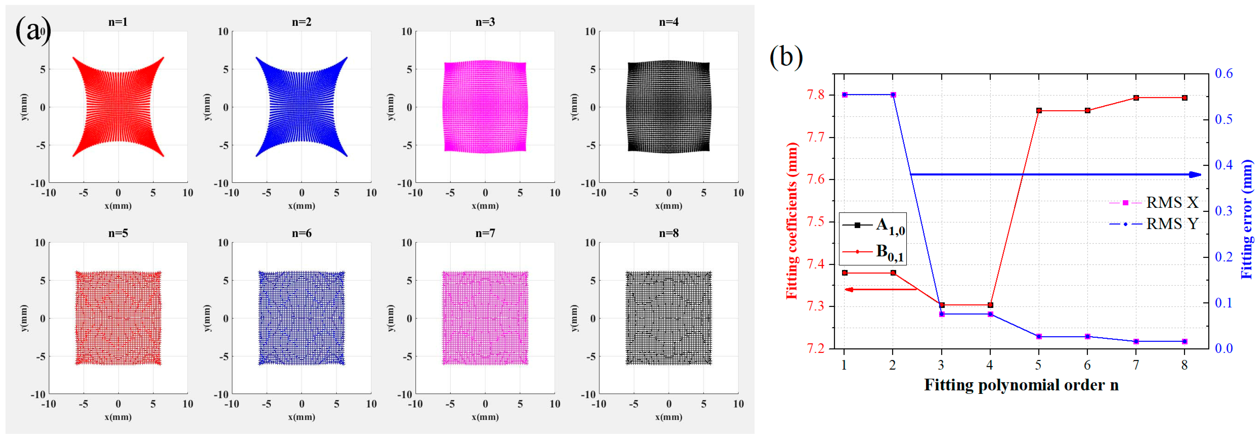
Figure 2.
Calibration results of the BPMs of the high-energy photon source (HEPS). (a) Position sensitivity coefficients of the 44 BPMs. (b) Other first-order coefficients. (c) Average and STD of coefficients for the 44 BPMs; the error bar in the figure corresponds to the STD of the 44 BPMs. (d) Position sensitivity coefficients of different types of the HEPS BPMs. The details of the BPMs can be found in reference [15].


Figure 3.
Fitting coefficients A1,0 and fitting errors with different scanning ranges inferred using the CST results.
Figure 3.
Fitting coefficients A1,0 and fitting errors with different scanning ranges inferred using the CST results.

Figure 4.
Fitting coefficient A1,0 and fitting errors with different scan steps calculated using the calibration results (xrange = 6 mm). (a) A1,0 with different step sizes for n = 1, 3, 5, 7. (b) Xerror with different step sizes for n = 3, 5, 7. (c) A1,0 with different steps for n = 1. (d) Xerror with different step sizes for n = 1.

Figure 5.
Fitting coefficients and errors with different scan steps inferred by the calibration results (xrange = 2 mm), adopting the same processing method as that in Figure 4. The points with step size multiples of 0.05 mm were selected for fitting. (a) A1,0 and B0,1 for n = 1, 3, 5, 7. (b) Xerror and Yerror for n = 1, 3, 5, 7.

Figure 6.
Fitting coefficients and errors with different scan steps inferred by the calibration results (xrange = 1 mm), adopting the same processing method as that in Figure 4. The points with step size multiples of 0.025 mm were selected for fitting. (a) A1,0 and B0,1 for n = 1, 3, 5, 7. (b) Xerror and Yerror for n = 1, 3, 5, 7.
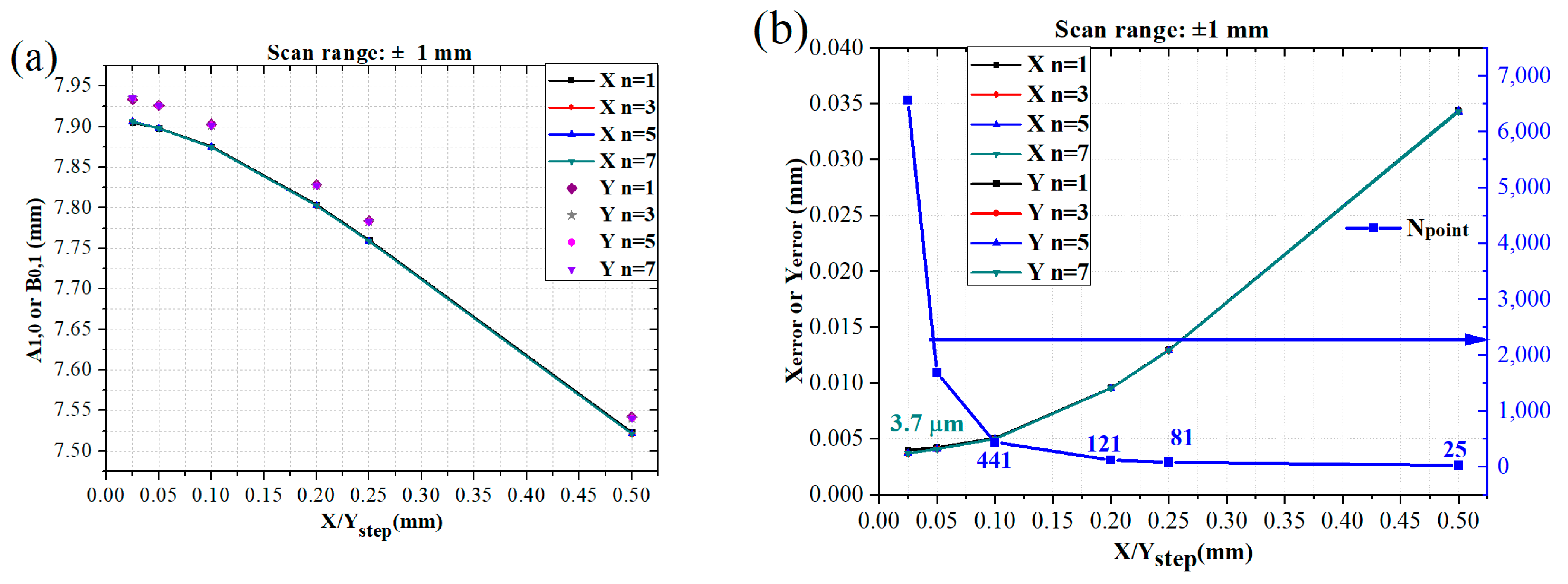
Figure 7.
Ball fiducials and buttons of the BPM.

Figure 8.
(a,b) Position deviation histogram for 1800 buttons and 2120 fiducials measured by CMM.


Table 1.
Fitting coefficients calculated by the CST simulation and calibration system (Unit: mm).
| n = 1 | n = 2 | n = 3 | n = 4 | |||||
|---|---|---|---|---|---|---|---|---|
| CST | G-Line | CST | G-Line | CST | G-Line | CST | G-Line | |
| A0,0 | 0.000038 | 0.003537 | 0.000030 | 0.006438 | 0.000023 | 0.006795 | 0.000014 | 0.007588 |
| A1,0 | 7.417378 | 7.418390 | 7.417378 | 7.421355 | 7.341290 | 7.338520 | 7.341290 | 7.340805 |
| A0,1 | 0.000040 | −0.019471 | 0.000040 | −0.019635 | 0.000691 | −0.026786 | 0.000694 | −0.027234 |
| A2,0 | / | −0.000056 | −0.006683 | 0.000072 | 0.001686 | −0.000004 | 0.005409 | |
| A1,1 | / | 0.000023 | 0.075334 | 0.000155 | 0.070936 | 0.000251 | 0.133496 | |
| A0,2 | / | 0.000090 | −0.007537 | 0.000044 | −0.012418 | 0.000206 | −0.017898 | |
| A3,0 | / | / | 7.570054 | 7.301139 | 7.570054 | 7.295493 | ||
| A2,1 | / | / | 0.001055 | 0.039867 | 0.001055 | 0.040914 | ||
| A1,2 | / | / | −8.575943 | −8.284103 | −8.575943 | −8.286623 | ||
| A0,3 | / | / | −0.002331 | −0.002462 | −0.002331 | −0.001646 | ||
| A4,0 | / | / | / | 0.000291 | −0.037322 | |||
| A3,1 | / | / | / | 0.000472 | −0.080949 | |||
| A2,2 | / | / | / | −0.000117 | 0.053807 | |||
| A1,3 | / | / | / | −0.000676 | −0.051802 | |||
| A0,4 | / | / | / | −0.000311 | −0.013570 | |||
Table 2.
Fitting error statistics for the 44 BPMs where the scan range, the step size, and Npoint are ±6 mm, 0.25 mm, and 2401.
Table 2.
Fitting error statistics for the 44 BPMs where the scan range, the step size, and Npoint are ±6 mm, 0.25 mm, and 2401.
| Xerror | ||||||||
| n = 1 | n = 2 | n = 3 | n = 4 | n = 5 | n = 6 | n = 7 | n = 8 | |
| Mean * (mm) | 0.54672 | 0.54507 | 0.07440 | 0.07348 | 0.02581 | 0.02548 | 0.01595 | 0.01589 |
| STD ** (μm) | 2.664 | 2.291 | 1.547 | 1.150 | 1.367 | 1.114 | 1.270 | 1.190 |
| STD/Mean (%) | 0.49 | 0.42 | 2.08 | 1.57 | 5.30 | 4.37 | 7.96 | 7.49 |
| Yerror | ||||||||
| n = 1 | n = 2 | n = 3 | n = 4 | n = 5 | n = 6 | n = 7 | n = 8 | |
| Mean (mm) | 0.54636 | 0.54479 | 0.07413 | 0.07349 | 0.02574 | 0.02537 | 0.01587 | 0.01579 |
| STD (μm) | 2.423 | 2.466 | 1.417 | 0.835 | 1.093 | 0.727 | 1.300 | 1.126 |
| STD/Mean (%) | 0.44 | 0.45 | 1.91 | 1.14 | 4.25 | 2.87 | 8.19 | 7.13 |
* Xerror was calculated by Equation (6), then the average value of 44 BPMs was calculated. ** The STD of 44 measured Xerror results.
Disclaimer/Publisher’s Note: The statements, opinions and data contained in all publications are solely those of the individual author(s) and contributor(s) and not of MDPI and/or the editor(s). MDPI and/or the editor(s) disclaim responsibility for any injury to people or property resulting from any ideas, methods, instructions or products referred to in the content. |
© 2024 by the authors. Licensee MDPI, Basel, Switzerland. This article is an open access article distributed under the terms and conditions of the Creative Commons Attribution (CC BY) license (https://creativecommons.org/licenses/by/4.0/).
Share and Cite
MDPI and ACS Style
He, J.; Sui, Y.; Liang, C.; Du, Y.; Zhao, Y.; Zhang, W.; Huang, F.; Xu, T.; Yue, J.; Cao, J. Preliminary Analysis of Beam Position Monitor Accuracy. Symmetry 2024, 16, 566. https://doi.org/10.3390/sym16050566
AMA Style
He J, Sui Y, Liang C, Du Y, Zhao Y, Zhang W, Huang F, Xu T, Yue J, Cao J. Preliminary Analysis of Beam Position Monitor Accuracy. Symmetry. 2024; 16(5):566. https://doi.org/10.3390/sym16050566
Chicago/Turabian StyleHe, Jun, Yanfeng Sui, Chongyang Liang, Yaoyao Du, Ying Zhao, Wan Zhang, Fangqi Huang, Taoguang Xu, Junhui Yue, and Jianshe Cao. 2024. "Preliminary Analysis of Beam Position Monitor Accuracy" Symmetry 16, no. 5: 566. https://doi.org/10.3390/sym16050566
Note that from the first issue of 2016, this journal uses article numbers instead of page numbers. See further details here.