
Sound Source Localization Method Based on Time Reversal Operator Decomposition in Reverberant Environments

1
State Key Laboratory of Integrated Service Network, Xidian University, Xi’an 710071, China
2
Collaborative Innovation Center of Information Sensing and Understanding, Xidian University, Xi’an 710071, China
*
Author to whom correspondence should be addressed.
Electronics 2024, 13(9), 1782; https://doi.org/10.3390/electronics13091782
Submission received: 3 April 2024
/
Revised: 28 April 2024
/
Accepted: 1 May 2024
/
Published: 5 May 2024
Abstract
:Predicting sound sources in reverberant environments is a challenging task because reverberation causes reflection and scattering of sound waves, making it difficult to accurately determine the position of the sound source. Due to the characteristics of overcoming multipath effects and adaptive focusing of the time reversal technology, this paper focuses on the application of the time reversal operator decomposition method for sound source localization in reverberant environments and proposes the image-source time reversal multiple signals classification (ISTR-MUSIC) method. Firstly, the time reversal operator is derived, followed by the proposal of a subspace method to achieve sound source localization. Meanwhile, the use of the image-source method is proposed to calculate and construct the transfer matrix. To validate the effectiveness of the proposed method, simulations and real-data experiments were performed. In the simulation experiments, the performance of the proposed method under different array element numbers, signal-to-noise ratios, reverberation times, frequencies, and numbers of sound sources were studied and analyzed. A comparison was also made with the traditional time reversal method and the MUSIC algorithm. The experiment was conducted in a reverberation chamber. Simulation and experimental results show that the proposed method has good localization performance and robustness in reverberant environments.
1. Introduction
Sound source localization (SSL) in reverberation environments is a long-standing and widely studied field, with strong demand in areas such as video conferencing, smart home, speech enhancement, etc. [1]. However, current algorithms cannot fully solve various limitations encountered in real-world applications. Therefore, SSL is still a highly challenging research direction.
The traditional SSL technology is based on microphone array, and there are three main algorithms, namely, beamforming [2], spatial spectrum estimation [3], and time difference of arrival estimation [4]. Additionally, the dual-microphone localization algorithm based on the binaural hearing mechanism is also studied. However, most of it remains theoretical, and its applications are mainly in near-field or high signal-to-noise ratio (SNR) scenarios. The aforementioned methods, along with continuously updated post-processing algorithms combined with specific arrays, can achieve good SSL results, thus finding wide applications in free-field environments. However, these methods also suffer from drawbacks such as algorithm complexity, the need for specialized array designs, high economic costs, and susceptibility to environmental factors like noise and reverberation. These limitations, to some extent, restrict their practical applications. Therefore, directly applying these methods for localization in complex enclosed environments like indoor sound fields has inherent deficiencies.
The prominent feature of the acoustic time reversal (TR) method derived from optical phase conjugation is its ability to overcome multipath effects [5], enabling adaptive focusing without the need for large arrays. Therefore, it is highly suitable for SSL in reverberant environments. This characteristic makes it also suitable for a variety of environments where multiple-path effects exist, such as medical imaging [6,7], through-wall imaging [8], seismic source localization [9], and radar imaging [10].
The detailed process of TR is as follows: Firstly, one or more sensors, typically microphones, are deployed inside the area where SSL is needed. These microphones are used to receive the acoustic signals present in the environment. The received signals include the direct arrival signal from the sound source as well as various multipath signals generated by reflections, refractions, and scattering. Next, the received signals are reversed in time, meaning that the signals received earlier are placed later on the time axis, while the signals received later are placed earlier on the time axis. This operation is typically carried out using digital signal processing techniques, often involving the reversal of both the amplitude and phase of the signals. The reversed signals are then retransmitted through the sensors. According to the principle of spatial reciprocity, the signals propagate along paths opposite to the original propagation direction, thus forming a focusing area in the environment resembling the original position of the sound source. Due to the effect of the time reversal, the signals in the focusing area overlap and reinforce each other, enhancing the signal intensity. By detecting changes in signal intensity within the focusing area, the position of the sound source can be determined. For the step of transmitting the signal after TR and then re-receiving it, it is usually simulated on a computer in reality; thus, it is called virtual time reversal (VTR), which greatly reduces the workload but requires that the simulated propagation channel be as close to the real propagation channel as possible.
Fink et al. experimentally verified the feasibility of the TR method in reverberation environments for the first time, but the obtained focal spot size was larger than 1/2 wavelength λ [11]. Draeger et al. conducted localization experiments in a reverberant silicon cavity using a single microphone and a pulsed signal with a center frequency of 1 MHz, achieving a resolution of λ/2 [12,13,14]. Fink et al. then selected a signal with a central frequency of 975 Hz as the sound source, and achieved SSL in an ordinary room using a uniform linear array containing 20 microphones, with a resolution still at λ/2 [15]. The initial research on the TR method primarily focused on validating its feasibility in reverberant environments. Most of these studies were conducted through laboratory experiments, involving sound sources with both high and low frequencies. Overall, early-stage research merely employed the TR method for SSL in reverberant environments, with spatial resolution limited to λ/2. Therefore, scholars then conducted research on how to improve the resolution of the method. Fink et al. proposed the concept of an acoustic sink to break through the λ/2 limitation [16]. Conti et al. surrounded the sound source completely with microphones, achieving a resolution of λ/20 in near-field [17]. Foroohar et al. designed a TR-based (DOA) estimator for radar waveform detection in strong multipath environments. Numerical simulations also confirmed the benefit of applying TR to SSL algorithms, especially at low SNR below 5 dB [18]. Mimani improved the resolution of the TR method by placing a reflecting surface and conducted simulation comparisons with the traditional beamforming method [19]. Ma et al. also achieved a resolution of λ/4 by placing objects, which were subwavelength scatterers [20]. Li proposed a cross-spectrum TR method corrected in the wavenumber domain. Numerical simulation and experimental results show that the spatial resolution of the proposed method can reach 1/34 λ at 100 Hz under a low SNR (0 dB) in the near field. Ma et al. proposed a TR–SBL method for low-frequency sound sources, which achieved good results in the environment of reverberation and low SNR [21].
Fink proposed the iterative time reversal (ITR) technique, which achieves the detection of targets with maximum scattering cross-section by iteratively repeating the TR signal operations [22]. Following this, he proposed the method of the decomposition of the time reversal operator (DORT) based on ITR processing. This method performs eigenvalue (singular value) decomposition on the TR operator, achieving selective focusing through the processing of eigenvectors. Both theoretical analysis and experimental results demonstrate its good localization performance for scatterers in inhomogeneous media [23]. Later, successful applications of the method were achieved to predict the position and size of α-phase grain defects in aerospace material titanium alloy [24].
Compared to DORT, multiple signal classification based on TR (TR-MUSIC) offers a complementary perspective. DORT is a signal subspace projection method, whereas the TR method, conversely, is a noise subspace projection method. In particular, the TR-MUSIC method works well as long as the noise space dimension exceeds the signal subspace dimension [25]. The TR-MUSIC method was first introduced for the Born approximated scattering linear model [26]. Later, it was found to be suitable for scenarios with multiple scatterers [27]. Domenico et al. studied the performance of the TR-MUSIC method in locating point-like scatterers in the presence of an additive noise destruction matrix [28]. Adaptive TR-MUSIC is proposed for low angle estimation with monostatic MIMO radar system [29]. The Lamb wave-based TR-MUSIC algorithm is introduced into the application of metal plate damage detection [30]. TR-MUSIC and phase-coherent form (PC-MUSIC) are explored in the nondestructive testing imaging of extended target machined in solids [31,32]. A novel imaging method called the cascaded TR-MUSIC is proposed to precisely locate multiple harmful radiated passive intermodulation sources [33]. A truncated TR operator-based imaging method is proposed; numerical results demonstrate that the method significantly decreases computational complexity and achieves better accuracy [34]. Various scenarios different from SSL were listed, partly to demonstrate the method’s applicability to a wide range of scenarios, and partly because there are few studies on this method in reverberation environments. However, the previously listed scenarios all involve multipath effects, similar to indoor reverberation, and the sound source is generally assumed to be a point. In view of its superiority in target localization in multipath environments, we introduced it into the study of SSL in reverberation environments.
Currently, when using the TR-MUSIC method for SSL, the channel response function h generally adopts either the Green’s function [33] or the steering vector [35] from the source to the receiver. However, in multipath environments, computing the Green’s function typically involves complex integrals and mathematical derivations, especially for complex boundary problems and geometric shapes, which can result in high computational costs. This makes computing the Green’s function in multipath environments in practical applications potentially require significant computational resources and time. The accuracy of the Green’s function is limited by the selected model and approximation methods, with poor adaptability. The steering vector function only considers the direct sound, neglecting later reflected sounds.
In view of the limitations of Green’s function and steering vector, we propose using the image-source method to compute the channel response function from the sound source to the receiver. The image-source method is commonly used for the analysis of the acoustic properties of enclosures, and the obtained channel response function is relatively accurate, and it does not require complex mathematical derivations or integral calculations; typically, it only involves replacing the real source point with a virtual point source. The specific derivation of this method can be found in Section 2.2.
The study is organized as follows. Section 2 discusses the SSL model in reverberant environments. Section 3 describes the numerical simulations performed to validate the proposed method. Section 4 reports the real-data experiments in a reverberation chamber and the analysis of the results. Finally, Section 5 presents the conclusion.
2. SSL Model in Reverberant Environments
2.1. DORT Process
The DORT algorithm is derived from the principle of iteration TR method. Firstly, the process of iteration TR is described by defining the transfer matrix, which consists of the channel response function, also known as the spatial impulse response (SIR), particularly in reverberant environments such as indoor settings, and the system is generally considered to be linear. The SSL system consists of two microphone arrays, each containing M microphones, one located not far from the sound source, and the other located at the sound source, which is simulated in the computer in reality; hence, it is called the virtual array. The array contains M array elements. The acoustic signal is s(t). SIR from the sound source to the m-th array element is represented by . The signal received by the m-th array element is
The symbol represents convolution, the length of the signal is ls, the length of the is lm, and the length of the corresponding received signal is lm + LS − 1. When you transform Equation (1) into the frequency domain
ω is the angular frequency. The TR operation t→−t in the time domain is equal to the phase conjugation in the frequency domain. Therefore, the TR form of Equation (2) is
The symbol * stands for conjugation. Then, the signal is re-transmitted back to the medium, and the array located at the position of the sound source will receive the signal again; that is, the matrix form of the signal obtained in the first iteration by the virtual array is
. N is the number of sound sources and M is the number of microphones.
In the second iteration, the signal received by the array is
The signal received by the array after 2n times of iteration TR is
is called TR operator (TRO). The ITR process is simulated on a computer, and this process is also completed on a computer in the subsequent experimental verification. The odd Rn is received by the virtual array, and the even Rn is received by the regular array.
According to the spatial reciprocity theorem, the SIR from the m-th element to the signal is the same as the SIR from the signal to the m-th element, so the transfer matrix has symmetry, and is Hermitian with positive eigenvalues. The size of the is M × M. The eigenvalue decomposition is performed on the TRO. There are N eigenvalues in total, , N is number of sound sources, and the corresponding eigenvectors are . The relation between and the eigenvectors can be written as
Signal S can be rewritten as the sum of eigenspace vectors:
After 2n + 1 of ITR, the output signal of the microphone array is
If n is large enough, the terms from to in Equation (9) can be neglected, simplifying to
As can be seen from Equation (10), after several ITR, the array can basically only receive the echo at the strongest signal reflection; that is, the signal can only focus on one signal in the end.
2.2. Proposed ISTR-MUSIC
Generally speaking, when there is background noise in the environment, then the vector expression of the signal received by the array is
NN is generally Gaussian white noise and is incoherent with the signal. N indicates the number of sound sources in line. H is the transfer matrix composed of SIR. Here, the image-source method is introduced to calculate hnm.
According to the principles of geometric acoustics, there exists a “virtual source” on the opposite side of each wall surface in an enclosed space, based on the symmetry of the sound source. This virtual source generates its own subsequent virtual sources, and so on, as shown in Figure 1. The energy of these virtual sources is determined by the absorption coefficient of the wall surface that generates them and their level. Once the positions and energies of all virtual sources are determined, the contribution of the sound source to the receiving point can be equivalently expressed as the sum of the contributions of these virtual sources. This is the basic idea behind the image-source method. This method yields relatively accurate results.
The coordinates of the sound source are (xs, ys, zs), and the coordinates of the m-th microphone are (xm, ym, zm). The distance traveled by the direct sound is given by the following equation:
Any virtual source and its original image-source, namely, the previous-level virtual source, exhibit a symmetrical relationship. Therefore, coordinates of a virtual source can be obtained based on geometric transformations of the previous-level virtual source. If the coordinates of the ith virtual source are represented as (xi, yi, zi), then the distance from it to the m-th microphone is calculated as
The sound pressure of the point away from the sound source d can be calculated as
The total sound pressure received by the m-th array element is
where q0 represents the initial sound pressure of the sound source and αi denotes the cumulative sound absorption coefficient for the i-th virtual source, which is equal to the product of the sound absorption coefficients of each wall forming the virtual source. Additionally, k represents the wave number.
The signal obtained after time reversal is
Q is the sound pressure calculated by the image-source method of Equation (15).
The covariance matrix of the re-received signal Z is
is the Hermitian transpose operator. RX(ω) is square matrix with the size of M × M. Performing singular value decomposition (SVD) on matrix RX(ω) yields
Us is signal subspace, Σs is the diagonal matrix corresponding to the larger eigenvalues, and when there are D signals, ; the corresponding eigenvector can be expressed as . UN is noise subspace, ΣN is the diagonal matrix corresponding to the smaller eigenvalues, ; the corresponding eigenvector can be expressed as . Since RX is a Hermite matrix, each eigenvector is mutually orthogonal; that is
The characteristic property of the subspace indicates that the space spanned by the SIR is the same as the signal subspace. Therefore, the eigenvectors of the SIR correspond to the spatial location information of the signal. Thus, the position of the sound source can be estimated based on the characteristic decomposition property.
Noise matrix is constructed by using the eigenvector of noise:
Then the spatial spectrum can be defined as
Due to the presence of background noise, the denominator of Equation (21) will not be equal to zero, but there will be a minimum value, resulting in a corresponding peak value, and the position corresponding to the peak value is considered to be the position of the sound source.
3. Simulations and Analysis
In this section, we first provide detailed simulation parameters. Next, we evaluate the performance against the traditional TR and MUSIC methods. Finally, we investigate the performance of the proposed ISTR-MUSIC method under various parameters, including the number of microphones, SNR, different sound absorption coefficient, and presence of multiple sound sources. These methods are implemented on the MATLAB R2022a platform running on a computer equipped with the following parameters: Intel (R) Core (TM) i7-13700KF CPU @3.40 GHz. The computer manufacturer is Intel, from Xi’an, China.
The steps of the simulation experiment are as follows:
- 1.
- The interested area is divided into n grids, and the grid spacing is set as dd, assuming that the sound source is located in the center of the grid;
- 2.
- The microphone positions are arranged, and the sound pressure Q of different grid points received by the array is calculated;
- 3.
- The signal received by the array is y, and it converts it to the frequency domain to obtain Y, performs conjugation processing, and then sends it back to the medium. The signal received by the virtual array is Z(ω);
- 4.
- The covariance matrix RX of Z(ω) is calculated, and the eigenvector EN corresponding to the noise subspace is obtained by singular value decomposition;
- 5.
- According to Equation (21), the final spatial spectrum is calculated, and the position corresponding to the maximum value is the position of the sound source.
3.1. Simulation Condition and Evaluation Index
3.1.1. Simulation Condition
A rectangular space of 6 m × 4 m × 3 m is selected as the enclosed space for research. The array is a uniform linear array, consisting of M = 20 array elements with a spacing of 0.1 m. The array is located on a 1 m high horizontal surface. In addition, the x-axis coordinate of the array is 0.9 + 0.1*m, m = 1, 2, …, M, and the y-axis coordinate of the array is 1.0; the units are in meters. Then, the possible position of the sound source is selected as the area of interest, and the region is divided into k grids. The area of interest is also located on a 1 m high plane. The coordinates on the x-axis range from 2.55 to 3.5, and on the y-axis, they range from 2.0 to 2.95; the total number of grids is 400. The grid spacing is 0.05 m, with a total of 400 grids. The signal utilizes sinusoidal signals of different frequencies, the duration is 10 s, and the sampling frequency is 2205 Hz. A sketch of the enclosed space with the position of the microphone array and grids is shown in Figure 2.
Assuming the sound absorption coefficient α of each surface is the same, the reverberation time T60 of the enclosed space is calculated according to the Ealing formula when the average absorption coefficient is greater than 0.2, as follows:
V is the volume; S is the surface area.
3.1.2. Evaluation Index (EI)
When the grid position predicted by the SSL algorithm is exactly the position of the sound source, the SSL result is considered correct. In this paper, we plan to use the following indexes to evaluate SSL performance of different methods.
- SSL error. When the localization result is accurate, the error is 0. When the result is inaccurate, the position obtained by the SSL algorithm is la, and the distance between the predicted position and the actual position ls is the error, . It intuitively reflects the spatial resolution of the SSL algorithm. The smaller e is, the better the algorithm performance is.
- Accuracy, represented by A. The total number of experiments is t, and the number of accurate results is c; thus, A = c/t × 100%. SSL accuracy can serve as an indicator of the reliability of SSL results. A higherHigher accuracy implies that the results are more reliable.
- Root mean square error (RMSE). It is an important index for measuring localization accuracy, representing the average deviation between observed values and true values. A lower RMSE value indicates better performance of the model, as it can get closer to the true values on average.
- Ratio of peak values, represented by P. The peak value of the correlation coefficient is p1 and the second peak value is p2, P = p2/p1. This index reflects the correlation between observed values and true values. A smaller value indicates better performance of the algorithm.
3.2. Comparison with Different Methods
In this section, firstly, we compare the performance of the proposed ISTR-MUSIC method, TR method, and MUSIC method. A narrowband signal with a frequency of 1000 Hz was chosen as the sound source. The room’s absorption coefficient is set to 0.4. The SSL results of grid point 150 predicted by the three methods are shown in Figure 3.
The information contained in Figure 3 is extensive; we will describe each one separately. In the localization maps formed by focusing imaging, the focal spot produced by the proposed ISTR-MUSIC method is relatively small, resulting in the clearest image, as shown in Figure 3a. The focal spot obtained through traditional TR is the largest. Although the focal spot obtained by the MUSIC method is not large, its sidelobe value is very high, which affects the display of the SSL result. The details of the SSL results are further compared in Figure 3d. The sidelobe value obtained by the proposed method is approximately −15 dB, while that obtained by the TR method is about −3 dB, which increased by 12 dB. Similarly, the sidelobe value obtained by the MUSIC method is about −7 dB, which increased by 8 dB. In summary, the proposed ISTR-MUSIC method exhibits a smaller sidelobe value and produces a clearer SSL map.
3.3. Studies in Different Situations
In this section, we will investigate the SSL results of different methods under various parameters to further validate the performance of the proposed ISTR-MUSIC methods. These parameters include the number of microphones, SNR, reverberation time T60, different frequencies, and multiple sound sources.
3.3.1. Different Number of Microphones
Firstly, we examine the SSL performance of different methods with varying numbers of microphones. The number of microphones M is selected as 5, 10, 15, and 20. We utilize the ratio of peak values P as the evaluation index, and the results are depicted in Figure 4.
As depicted in Figure 4, the proposed ISTR-MUSIC method consistently demonstrates the smallest ratio of peak values P, approximately 0.05, irrespective of the number of microphones. When the array contains 5 and 10 microphones, the P obtained by the TR method is less than that of the MUSIC method (approximately 0.3). However, for arrays with more than 10 microphones, the ratio of peak P obtained by the TR method is larger than that of the MUSIC method (approximately 0.25). On the whole, a higher number of microphones correlates with a lower ratio of peak values, indicating better SSL performance.
3.3.2. Different SNRs
The SSL performance of the algorithm at low SNR is a crucial metric for evaluating its effectiveness. Therefore, we conducted a study on the method’s results at various SNR levels and compared them with two other methods. The SNR values were set to −15 dB, −10 dB, −5 dB, 0 dB, 5 dB, and 10 dB, while the number of microphones was fixed at 20. Each of the three algorithms underwent 30 Monte Carlo experiments, and the results were compiled and analyzed for RMSE, as illustrated in Figure 5.
As evident from Figure 5, in the case of a low SNR of −15 dB, the RMSE obtained by the proposed ISTR-MUSIC method is the smallest, approximately 0.4 m, whereas the TR method exhibits the largest, at around 0.8 m. The RMSE of the MUSIC method falls between the values of the other two methods, at approximately 0.6 m. In scenarios with SNR values of −10 dB, −5 dB, and 0 dB, the proposed method yields a decreasing RMSE, gradually reducing to 0.07 m as the SNR increases. The results of the MUSIC method gradually decrease to 0.3 m. However, the RMSE of the TR method exhibits a significant drop, reaching 0 directly. When the SNR exceeds 5 dB, the RMSE of both the proposed ISTR-MUSIC method and the TR method becomes 0, whereas for the MUSIC method, it remains at 0.2 m.
3.3.3. Different Reverberation Time
In enclosed spaces, reverberation reflects the sound reflection and attenuation within the environment. With a fixed volume, the reverberation time is determined by the absorption coefficient. We conducted an investigation into the localization performance under different absorption coefficients. The array consists of 20 microphones, with an SNR of 20 dB. Considering that the method is applied to meeting rooms, living rooms and other places, which may contain decorations with high sound absorption coefficients, such as carpets, glass, sofas, soft chairs, etc., a higher sound absorption coefficient is selected for verification. The absorption coefficients α are set to 0.3, 0.4, 0.5, and 0.6, and the corresponding reverberation time T60 is 300.9 ms, 210.1 ms, 154.8 ms, and 117.1 ms, respectively. The results are shown in Figure 6.
There is a lot of information contained in Figure 6, and we will describe it one by one. It can be clearly seen from Figure 6 that when the absorption coefficient is at its minimum value of 0.3, the sidelobe value in the obtained localization results is the largest. When the absorption coefficient is at its maximum value of 0.6, the sidelobe value in the obtained localization results is the smallest. When the absorption coefficient is 0.4 and 0.5, the sidelobe values are the third largest and the second largest, respectively. Although the sidelobe values obtained by the proposed ISTR-MUSIC method vary under different absorption coefficients, they are all very sharp, indicating that the proposed method has good localization performance in reverberant environments.
3.3.4. Different Frequencies
We also investigate the proposed ISTR-MUSIC method’s performance across various frequencies. Our study particularly emphasizes medium and low-frequency sound sources. The frequencies examined are 125 Hz, 250 Hz, 500 Hz, and 1000 Hz. The RMSE resulting from 30 Monte Carlo experiments is presented in Table 1.
Table 1 indicates that as the frequency of the sound source increases, the RMSE obtained by the proposed ISTR-MUSIC method gradually decreases. Specifically, the RMSE for the sound source at 1000 Hz is reduced by 60% compared to the source at 125 Hz. The RMSE of the localization results for the sound source at a frequency of 250 Hz increased by only 0.0038 m, which is 1.2%. The RMSE of the localization results for the sound source at a frequency of 500 Hz increased by 0.08 m, which is 29%.
3.3.5. Multiple Sound Sources
The proposed method exhibits clear advantages in the environment with multiple sound sources, assuming three sound sources with a frequency of 1000 Hz, and other conditions remaining as described above. The SSL results of the three methods are illustrated in Figure 7.
Firstly, from an overall perspective, all three methods are able to accurately predict the positions of the dual sound sources to varying degrees. It is evident that the spot size obtained by the TR method is larger than that of the other two methods. The spot size obtained by the proposed ISTR-MUSIC method is similar to that obtained by the MUSIC method, but the localization map of the MUSIC method exhibits a larger and more prominent sidelobe.
4. Real-Data Experiments
To validate the robustness of the proposed method, we conducted experiments in real-world environments. The specific environments and experimental procedures will be detailed in the following sections.
The experiments were conducted in a reverberation chamber with dimensions of 3.2 m × 5.7 m × 4.8 m. The floor of the reverberation chamber is covered with regular tiles, and the remaining five sides are white walls. The average sound absorption coefficient is set at 0.3. The measured reverberation time T60 is 2.6 s.
The array adopts a uniform linear configuration, comprising a total of 15 omnidirectional microphones, with a 4938 type of 4938 (Brüel & Kjær, Copenhagen, Denmark) and frequency response range of 4 Hz to 70 kHz. A certain corner of the chamber serves as the origin of the Cartesian coordinate system. The array is located on a horizontal plane at a height of 1.4 m, evenly distributed along the x-axis from 1.0 m to 2.4 m at intervals of 0.1 m, with a y-axis coordinate of 1.6 m. The sounding device is a spherical sound source with a diameter of 0.5 m, and the receiver is the Pulse 3060 module. Both devices are manufactured by Brüel & Kjær. The spherical sound source is placed at six different positions on a plane at a height of 1.4 m for emission, with coordinates (2.0, 2.1) m, (1.4, 2.1) m, (2.0, 3.3) m, (1.4, 3.3) m, (2.0, 4.5) m, and (1.4, 4.5) m. The Pulse device and the computer are positioned along the wall edge to minimize interference with sound reception. The region of interest in the reverberation chamber spans from 1.4 m to 2.0 m along the x-axis, from 2.1 m to 4.5 m along the y-axis, and at a height of 1.4 m along the z-axis. The space along the y-axis ranges from 2.1 m to 4.5 m, and along the z-axis, it is at a height of 1.4 m, divided into 175 grids with a spacing of 0.1 m for research purposes. The equipment layout in the reverberation chamber is shown in Figure 8a, while the schematic diagram of grid division and overall layout is presented in Figure 8b.
Consistent with the simulation, signals at frequencies of 125 Hz, 250 Hz, 500 Hz, and 1000 Hz are still chosen as the sound sources. Taking the sound source at (2.0, 3.3) m as an example, the SSL results of the proposed ISTR-MUSIC method are shown in Figure 9.
As can be seen from Figure 9, the localization map of the sound source with a frequency of 1000 Hz is the clearest. The localization results of the remaining three frequency sources are slightly more ambiguous than those of the 1000 Hz source, but the actual positions of the sources can still be distinguished. Overall, the proposed ISTR-MUSIC method shows the highest sidelobe value in the localization results for sound source with a frequency of 500 Hz.
Then, we process the signals collected from six different positions using the proposed ISTR-MUSIC method and evaluate the performance using RMSE as the performance evaluation index. The results are shown in Table 2.
Table 2 shows that when the frequency of the sound source is at the lowest 125 Hz, the RMSE obtained by the proposed method is the largest, which is 0.41 m; when the frequency of the sound source is at the highest 1000 Hz, the corresponding RMSE is the smallest, 0.17 m, which is reduced by 59%. RMSE for sound sources with frequencies of 250 Hz and 500 Hz are 0.34 m and 0.24 m, respectively, which are 17% and 41% lower than the RMSE for the lowest frequency. In general, the value of RMSE is inversely proportional to the frequency, and the higher the frequency, the smaller the RMSE of the sound source.
5. Conclusions
A novel ISTR-MUSIC method is proposed for localizing mid–low frequency sound sources in reverberant environments. The proposed method fully utilizes the anti-reverberation characteristics of the time reversal method and the high-resolution advantages of the MUSIC method. In our method, the singular value decomposition method is used to obtain the signal subspace and noise subspace for the time reversal operator, and the transfer matrix is calculated using the image-source method. The effectiveness of the proposed ISTR-MUSIC method has been verified through simulation experiments. Firstly, by comparing it with the traditional time reversal method and the MUSIC method, the advantages of this method are demonstrated in the reverberant environments. Then, the SSL performance of the proposed ISTR-MUSIC method under different conditions is studied in detail. The results indicate that the proposed method achieves satisfactory spatial resolution and strong robustness in the reverberation environment with fewer array elements and lower SNR. The real-data experiment was carried out in the reverberation chamber to localize the sound source through the proposed ITR-MUSIC method. The experimental results indicate that the ISTR-MUSIC method has a small RMSE in practical environments. All evidence indicate the effectiveness of the ISTR-MUSIC method for sound source localization in reverberant environments.
Author Contributions
Conceptualization, H.M.; methodology, H.M.; software, H.M.; validation, H.M.; formal analysis, H.M.; investigation, G.L. and Z.L.; resources, G.L.; data curation, H.M.; writing—original draft preparation, H.M.; writing—review and editing, H.M.; visualization, H.M.; supervision, T.S.; project administration, T.S.; funding acquisition, Z.L. All authors have read and agreed to the published version of the manuscript.
Funding
This work was funded by the National Natural Science Foundation of China, grant number 62001286.
Data Availability Statement
The data that support the findings of this study are available from the corresponding author, upon reasonable request.
Conflicts of Interest
The authors declare no conflicts of interest.
References
- Pierre-Amaury Grumiaux, S.D.K.C. A review of sound source localization with deep learning methods. arXiv 2021, arXiv:2109.03465. [Google Scholar]
- He, C.; Cheng, S.; Zheng, R.; Liu, J. Delay-and-sum beamforming based spatial mapping for multi-source sound localization. IEEE Internet Things 2024, 11, 16048–16060. [Google Scholar] [CrossRef]
- Meng, X.; Cao, B.; Yan, F.; Greco, M.; Gini, F.; Zhang, Y. Real-valued MUSIC for efficient direction of arrival estimation with arbitrary arrays: Mirror suppression and resolution improvement. Signal Process 2023, 202, 108766. [Google Scholar] [CrossRef]
- Simon, G. Acoustic Moving Source Localization using Sparse Time Difference of Arrival Measurements. In Proceedings of the IEEE 22nd International Symposium on Computational Intelligence and Informatics and 8th IEEE International Conference on Recent Achievements in Mechatronics, Automation, Computer Science and Robotics, Zhuhai, China, 26–28 June 2022. [Google Scholar]
- Osamu, I. An image-source reconstruction algorithm using phase conjugation for diffraction-limited imaging in an inhomogeneous medium. J. Acoust. Soc. Am. 1989, 85, 1602–1606. [Google Scholar]
- Xanthos, L.; Yavuz, M.; Himeno, R.; Yokota, H.; Costen, F. Resolution enhancement of uwb time-reversal microwave imaging in dispersive environments. IEEE Trans. Comput. Imaging 2021, 7, 925–934. [Google Scholar] [CrossRef]
- Haghpanah, M.; Kashani, Z.G.; Param, A.K. Breast cancer detection by time-reversal imaging using ultra-wideband modified circular patch antenna array. In Proceedings of the 2022 30th International Conference on Electrical Engineering, Seoul, South Korea, 17–19 May 2022. [Google Scholar]
- Sadeghi, S.; Mohammadpour-Aghdam, K.; Faraji-Dana, R.; Burkholder, R.J. A DORT-uniform diffraction tomography algorithm for through-the-wall imaging. IEEE Trans. Antennas Propag. 2020, 68, 3176–3183. [Google Scholar] [CrossRef]
- Li, F.; Bai, T.; Nakata, N.; Lyu, B.; Song, W. Efficient seismic source localization using simplified gaussian beam time reversal imaging. IEEE Trans. Geosci. Remote Sens. 2020, 58, 4472–4478. [Google Scholar] [CrossRef]
- Li, M.; Xi, X.; Song, Z.; Liu, G. Multitarget time-reversal radar imaging method based on high-resolution hyperbolic radon transform. IEEE Trans. Geosci. Remote Sens. 2022, 19, 1–5. [Google Scholar] [CrossRef]
- Cassereau, D.; Wu, F.; Fink, M. Limits of self-focusing using closed time-reversal cavities and mirrors-theory and experiment. In Proceedings of the IEEE Symposium on Ultrasonics, Honolulu, HI, USA, 4–7 December 1990. [Google Scholar]
- Draeger, C.; Fink, M. One-channel time reversal of elastic waves in a chaotic 2d-silicon cavity. Phys. Rev. Lett. 1997, 79, 407–410. [Google Scholar] [CrossRef]
- Draeger, C.; Aime, J.C.; Fink, M. One-channel time-reversal in chaotic cavities: Experimental results. J. Acoust. Soc. Am. 1999, 2, 618–625. [Google Scholar] [CrossRef]
- Draeger, C.; Fink, M. One-channel time-reversal in chaotic cavities: Theoretical limits. J. Acoust. Soc. Am. 1999, 105, 611–617. [Google Scholar] [CrossRef]
- Yon, S.; Tanter, M.; Fink, M. A Sound focusing in rooms: The time-reversal approach. J. Acoust. Soc. Am. 2003, 113, 1533–1543. [Google Scholar] [CrossRef] [PubMed]
- Bavu, E.; Besnainou, C.; Gibiat, V.; de Rosny, J.; Fink, M. Subwavelength sound focusing using a time-reversal acoustic sink. Acta Acust. United Acust. 2007, 93, 706–715. [Google Scholar]
- Conti, S.G.; Roux, P.; Kuperman, W.A. Near-field time-reversal amplification. J. Acoust. Soc. Am. 2007, 121, 3602–3606. [Google Scholar] [CrossRef] [PubMed]
- Foroozan, F.; Asif, A. Time reversal based active array source localization. IEEE Trans. Signal Process. 2011, 59, 2655–2668. [Google Scholar] [CrossRef]
- Mimani, A.; Porteous, R.; Doolan, C.J. A simulation-based analysis of the effect of a reflecting surface on aeroacoustic time-reversal source characterization and comparison with beamforming. Wave Motion 2017, 70, 65–89. [Google Scholar] [CrossRef]
- Ma, C.; Kim, S.; Fang, N.X. Far-field acoustic subwavelength imaging and edge detection based on spatial filtering and wave vector conversion. Nat. Commun. 2019, 10, 204. [Google Scholar] [CrossRef] [PubMed]
- Ma, H.; Shang, T.; Li, G.; Li, Z. Low-frequency sound source localization in enclosed space based on time reversal method. Measurement 2022, 204, 112096. [Google Scholar] [CrossRef]
- Prada, C.; Wu, F.; Fink, M. The iterative time reversal mirror: A solution to self-focusing in the pulse echo mode. J. Acoust. Soc. Am. 1991, 90, 1119–1129. [Google Scholar] [CrossRef]
- Prada, C.; Manneville, S.; Spoliansky, D.; Fink, M. Decomposition of the time reversal operator: Detection and selective focusing on two scatterers. J. Acoust. Soc. Am. 1996, 99, 2067–2076. [Google Scholar] [CrossRef]
- Bilski, P.; Panich, A.M.; Sergeev, N.A.; Wąsicki, J. Simple two-pulse time-reversal sequence for dipolar and quadrupolar-coupled spin systems. Solid State Nucl. Mag. 2004, 25, 76–79. [Google Scholar] [CrossRef] [PubMed]
- Yavuz, M.E.; Teixeira, F.L. Space-frequency ultrawideband time-reversal imaging. IEEE Trans. Geosci. Remote Sens. 2008, 46, 1115–1124. [Google Scholar] [CrossRef]
- Devaney, A.J. Time reversal imaging of obscured targets from multistatic data. IEEE Trans. Antennas Propag. 2005, 53, 1600–1610. [Google Scholar] [CrossRef]
- Marengo, E.A.; Gruber, F.K. Subspace-based localization and inverse scattering of multiply scattering point targets. Eurasip. J. Adv. Sig. Process. 2007, 1, 017342. [Google Scholar] [CrossRef]
- Ciuonzo, D.; Romano, G.; Solimene, R. Performance analysis of time-reversal MUSIC. IEEE Trans. Signal Process. 2015, 63, 2650–2662. [Google Scholar] [CrossRef]
- Tan, J.; Nie, Z.; Peng, S. In adaptive time reversal MUSIC algorithm with monostatic MIMO radar for low angle estimation. In Proceedings of the 2019 IEEE Radar Conference, Boston, MA, USA, 22–26 April 2019. [Google Scholar]
- He, J.; Yuan, F.; Chimenti, D.E.; Bond, L.J. Lamb waves based fast subwavelength imaging using a DORT-MUSIC algorithm. In Proceedings of the Aip Conference Proceedings, Terchova, Slovakia, 12–14 October 2016. [Google Scholar]
- Fan, C.; Yang, L.; Zhao, Y. Ultrasonic multi-frequency time-reversal-based imaging of extended targets. NDT E Int. 2020, 113, 102276. [Google Scholar] [CrossRef]
- Fan, C.; Yu, S.; Gao, B.; Zhao, Y.; Yang, L. Ultrasonic time-reversal-based super resolution imaging for defect localization and characterization. NDT E Int. 2022, 131, 102698. [Google Scholar] [CrossRef]
- Cheng, Z.; Li, X.; Liu, S.; Ma, M.; Liang, F.; Zhao, D.; Wang, B. Cascaded Time-Reversal-MUSIC approach for accurate location of passive intermodulation sources activated by antenna array. IEEE Trans. Antennas Propag. 2023, 71, 8841–8853. [Google Scholar] [CrossRef]
- Cheng, Z.; Ma, M.; Liang, F.; Zhao, D.; Wang, B. Low complexity time reversal imaging methods based on truncated time reversal operator. IEEE Trans. Geosci. Remote Sens. 2024, 62, 1. [Google Scholar] [CrossRef]
- Xu, C.; Wang, J.; Yin, S.; Deng, M. A focusing MUSIC algorithm for baseline-free Lamb wave damage localization. Mech. Syst. Signal Process. 2022, 164, 108242. [Google Scholar] [CrossRef]
Figure 1.
Image-source method diagram. (a) Room model. (b) First-order virtual source.

Figure 2.
Sketch of the enclosed space with the position of the array and grids.
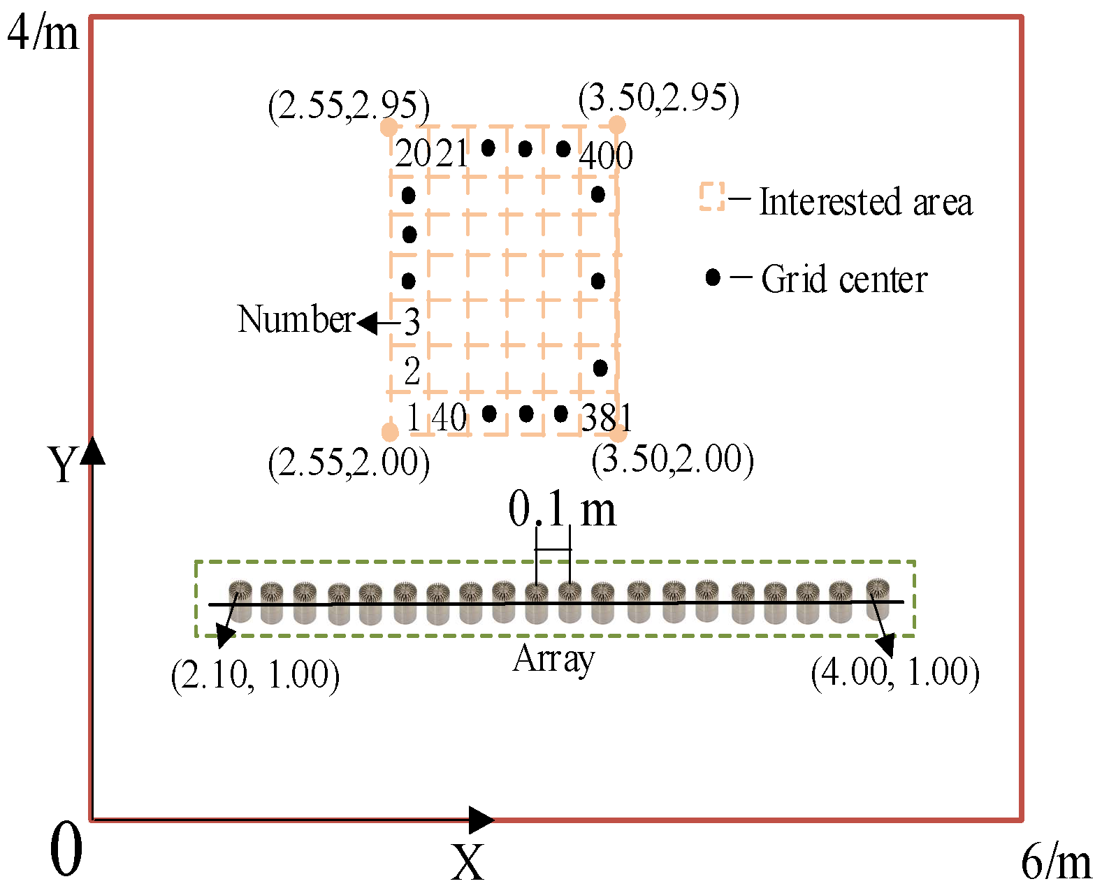
Figure 3.
The results of different methods. (a) Proposed ISTR-MUSIC method; (b) TR method; (c) MUSIC method; (d) Comparison of the three methods.
Figure 3.
The results of different methods. (a) Proposed ISTR-MUSIC method; (b) TR method; (c) MUSIC method; (d) Comparison of the three methods.

Figure 4.
The ratio of peak values P for different methods with varying numbers of microphones.

Figure 5.
RMSE under different SNRs.

Figure 6.
SSL results under different absorption coefficients.

Figure 7.
The dual-source localization results obtained from different methods. (a) ISTR-MUSIC method; (b) TR method; (c) MUSIC method.
Figure 7.
The dual-source localization results obtained from different methods. (a) ISTR-MUSIC method; (b) TR method; (c) MUSIC method.

Figure 8.
Overall layout of experimental equipment and the reverberation chamber. (a) Equipment layout; (b) Schematic diagram.
Figure 8.
Overall layout of experimental equipment and the reverberation chamber. (a) Equipment layout; (b) Schematic diagram.

Figure 9.
SSL result of the sound source at (2.0, 3.3) m. (a) Sound source with the frequency of 125 Hz; (b) Sound source with the frequency of 250 Hz; (c) Sound source with the frequency of 500 Hz; (d) Sound source with the frequency of 1000 Hz.
Figure 9.
SSL result of the sound source at (2.0, 3.3) m. (a) Sound source with the frequency of 125 Hz; (b) Sound source with the frequency of 250 Hz; (c) Sound source with the frequency of 500 Hz; (d) Sound source with the frequency of 1000 Hz.


Table 1.
RMSE under different frequencies.
| f/Hz | RMSE/m |
|---|---|
| 125 | 0.2953 |
| 250 | 0.2915 |
| 500 | 0.2110 |
| 1000 | 0.1173 |
Table 2.
RMSE of sound sources with different frequencies.
| f/Hz | RMSE/m |
|---|---|
| 125 | 0.41 |
| 250 | 0.34 |
| 500 | 0.24 |
| 1000 | 0.17 |
Disclaimer/Publisher’s Note: The statements, opinions and data contained in all publications are solely those of the individual author(s) and contributor(s) and not of MDPI and/or the editor(s). MDPI and/or the editor(s) disclaim responsibility for any injury to people or property resulting from any ideas, methods, instructions or products referred to in the content. |
© 2024 by the authors. Licensee MDPI, Basel, Switzerland. This article is an open access article distributed under the terms and conditions of the Creative Commons Attribution (CC BY) license (https://creativecommons.org/licenses/by/4.0/).
Share and Cite
MDPI and ACS Style
Ma, H.; Shang, T.; Li, G.; Li, Z. Sound Source Localization Method Based on Time Reversal Operator Decomposition in Reverberant Environments. Electronics 2024, 13, 1782. https://doi.org/10.3390/electronics13091782
AMA Style
Ma H, Shang T, Li G, Li Z. Sound Source Localization Method Based on Time Reversal Operator Decomposition in Reverberant Environments. Electronics. 2024; 13(9):1782. https://doi.org/10.3390/electronics13091782
Chicago/Turabian StyleMa, Huiying, Tao Shang, Gufeng Li, and Zhaokun Li. 2024. "Sound Source Localization Method Based on Time Reversal Operator Decomposition in Reverberant Environments" Electronics 13, no. 9: 1782. https://doi.org/10.3390/electronics13091782
Note that from the first issue of 2016, this journal uses article numbers instead of page numbers. See further details here.