Mathematical Model and Analysis of Novel Bevel Gear with High Load-Capacity Based on the Geometric Elements

Abstract

Load-capacity has always been one of the performances that is paid much attention to in the development of bevel gear transmission applications. Consequently, the mathematical model of novel bevel gear with high load-capacity based on geometric elements is proposed in this paper, which could be applied to the aviation, aerospace and other fields. In parallel, the design principle and design method of the novel bevel gear are introduced in detail. Subsequently, the conditions for tooth surface continuity and non-interference are derived. Furthermore, the model of novel bevel gear is established. Finally, the load-bearing characteristics are analyzed, revealing that an increase in the number of contact points could significantly enhance the load capacity of the bevel gear pairs. When the load torque applied to bevel gear II is 100 Nm, the contact pressure endured by the bevel gear pair with five-point contact is decreased by 41.37% compared to the bevel gear pair with single-point contact. When the number of contact points is the same, increasing the distance between the contact points could also reduce the contact stress. This provides strong theoretical support for the application of the bevel gear based on the geometric elements.

1. Introduction

The bevel gear is an important fundamental mechanical component, which is widely used in various engineering fields, such as automobiles, aerospace, and marine industries [1]. In response to the increased performance demands placed on bevel gear transmission pairs, scholars have embarked on relevant research endeavors [2,3,4,5], especially in terms of the load-carrying performance of bevel gear. Kong proposed a data-oriented loaded contact pressure regulation model, in order to monitor the meshing transmission performance and improve loaded contact fatigue life [6]. Based on multi-tooth deformation compatibility, Li put forward a numerical approach to predict the load distribution of a spiral bevel gear, based on multi-tooth deformation compatibility. This approach specifically addresses the contact pressure of the spiral bevel gear [7]. Mu put forth an innovative higher-order tooth surface modification method, which could be used to reduce the vibration excitation of gear transmission [8]. Song introduced a sensitive misalignment-oriented model for regulating contact pressure, providing crucial insights into the monitoring of meshing transmission performance [9]. To achieve precise and numerically efficient tooth contact analysis, Vivet developed a penetration-based gear contact model for spiral bevel gears [10]. For both static and dynamic simulations of bevel gears, A. Pigé proposed an innovative mesh interface model. The results demonstrated that load significantly impacts the contact conditions in bevel gears [11]. Batsch presented a mathematical model of convex-concave helical bevel gear mesh, aiming to increase the instantaneous contact area and consequently reduce the contact stress value [12]. Han proposed the nonlinear dynamic model to predict the skidding behavior [13]. Chen constructed the coupling model of mixed elastohydrodynamic transient lubrication and time-varying wear [14], and Shi analyzed the transient time-varying load to explore the thermal-pressure coupled effects under the actual operating conditions [15].

The most developed and extensively utilized tooth surface design method for spiral bevel gears is the conjugate surface meshing theory combined with local synthesis approach [16,17,18,19]. Conjugate surface meshing theory still plays a dominant role in the research of gear meshing theory. However, with the advancement of technology and to meet higher performance requirements of spiral bevel gear transmission mechanisms in industrial fields, many scholars are also proposing new meshing theory and continuously developing them in recent years. Chen proposed meshing theory based on geometric elements [20,21,22]. Geometric elements refer to points, curves, and surfaces, which are the three basic elements. Every combination of two of these elements forms a pair of contact relationships. Surface conjugation is one of the contact relationships, and compared to surface conjugation, curve conjugation is more diverse. Compared with general arc tooth bevel gears, bevel gears based on geometric elements could yield precise tooth surface equations and contact areas based on predetermined conjugate curves and tooth profile. Currently, such bevel gears are not suitable for applications requiring low tooth surface hardness. In order to enhance the load-carrying capacity of geometrically designed gears with soft tooth surfaces, Tan put forward a design method for bevel gears with single-point contact [23,24], and Liang developed the design method for gears based on curves elements with double contact points and three contact points [25,26]. Research by scholars has found that the gear based on the geometric elements can enhance tooth surface load-carrying capacity by increasing the number of contact points. However, the current primary research focuses on the three-point contact form, and gear designs with more than three-point contact have not yet been proposed. Therefore, the general design method for the bevel gear with multi-point contact is presented, which can be used for designing from single-point to multi-point contact.

In this paper, the general design method for the novel bevel gear pair with high load-capacity based on geometric elements is proposed, and the mathematical model is established. Subsequently, the tooth surface contact characteristics are investigated. Finally, the load-bearing characteristics of the novel bevel gear pair based on the geometric elements are analyzed.

2. Design Principle of Bevel Gear Based on the Geometric Elements

2.1. The Principle of Conjugate Curve

The design principle of the bevel gear based on geometric elements is illustrated in Figure 1. The principle of conjugate curve is introduced in this section. The design of tooth profile and tooth surface construction are discussed in the third section.

The conjugate curve could be characterized as a pair of smooth curves, following a prescribed motion law, which maintain continuous tangential contact along the specified direction throughout their motion, as shown in Figure 2. At each moment, curves Γ_I and Γ_II are in point contact, meaning they are tangentially touching at the contact point H. When the relative motion is specified, not only is curve Γ_II the conjugate curve of curve Γ_I but curve Γ_I is also the conjugate curve of curve Γ_II within a certain range.

2.2. Applied Coordinate System

According to the actual situation of the bevel gear drive and for the convenience of subsequent derivations, the coordinate system is established as shown in Figure 3. Coordinate systems S₀(O₀-x₀,y₀,z₀) and S_p(O_p-x_p,y_p,z_p) are two orthogonal right-handed coordinate systems fixed in space, where the z₀-axis coincides with the rotation axis of bevel gear I and the z_p-axis coincides with the rotation axis of bevel gear II. The shaft angle between the two revolving axles of these two bevel gears is ψ.

Additionally, coordinate systems S_I(O_I-x_I,y_I,z_I) and S_II(O_II-x_II,y_II,z_II) are respectively fixed to be right-handed orthogonal coordinate systems on bevel gear I and bevel gear II. At the initial position, they coincide respectively with coordinate systems S₀(O₀-x₀,y₀,z₀) and S_p(O_p-x_p,y_p,z_p). Bevel gear I rotates around the z₀-axis with a constant angular velocity ω_I, while bevel gear II rotates around the z_p-axis with a constant angular velocity ω_II. After a certain period of time from the initial position, coordinate systems S_I(O_I-x_I,y_I,z_I) and S_II(O_II-x_II,y_II,z_II) move to the illustrated positions, ϕ_I and ϕ_II represent the angles that bevel gear I and bevel gear II have rotated through, respectively.

The transformation relationship between coordinate systems S₀(O₀-x₀,y₀,z₀) and S_I(O_I-x_I,y_I,z_I) is described as:

$${\mathit{R}}_{0\mathrm{I}}=\left[\begin{array}{cccc}\cos {\varphi }_{\mathrm{I}}& -\sin {\varphi }_{\mathrm{I}}& 0& 0\\ \sin {\varphi }_{\mathrm{I}}& \cos {\varphi }_{\mathrm{I}}& 0& 0\\ 0& 0& 1& 0\\ 0& 0& 0& 1\end{array}\right]$$

(1)

The transformation relationship between coordinate systems S_p(O_p-x_p,y_p,z_p) and S₀(O₀-x₀,y₀,z₀) is described as:

$${\mathit{R}}_{\mathrm{p}0}=\left[\begin{array}{cccc}1& 0& 0& 0\\ 0& \cos \psi & -\sin \psi & 0\\ 0& \sin \psi & \cos \psi & 0\\ 0& 0& 0& 1\end{array}\right]$$

(2)

The transformation relationship between coordinate systems S_II(O_II-x_II,y_II,z_II) and S_p(O_p-x_p,y_p,z_p) is described as:

$${\mathit{R}}_{\mathrm{IIp}}=\left[\begin{array}{cccc}\cos {\varphi }_{\mathrm{II}}& -\sin {\varphi }_{\mathrm{II}}& 0& 0\\ \sin {\varphi }_{\mathrm{II}}& \cos {\varphi }_{\mathrm{II}}& 0& 0\\ 0& 0& 1& 0\\ 0& 0& 0& 1\end{array}\right]$$

(3)

According to the principle of coordinate transformation, the transformation relationship between coordinate systems S_II(O_II-x_II,y_II,z_II) and S_I(O_I-x_I,y_I,z_I) is obtained:

$${\mathit{R}}_{\text{II-I}}={\mathit{R}}_{\mathrm{IIp}}\cdot {\mathit{R}}_{\mathrm{p}0}\cdot {\mathit{R}}_{0\mathrm{I}}$$

(4)

Substituting Equations (1)–(3) into (4), ${\mathit{R}}_{\text{II-I}}$ is expressed as:

$${\mathit{R}}_{\text{II-I}}=\left(\begin{array}{cccc}\cos {\varphi }_{\mathrm{I}}\cos {\varphi }_{\mathrm{II}}-\cos \psi \sin {\varphi }_{\mathrm{I}}\sin {\varphi }_{\mathrm{II}}& -\sin {\varphi }_{\mathrm{I}}\cos {\varphi }_{\mathrm{II}}-\cos \psi \cos {\varphi }_{\mathrm{I}}\sin {\varphi }_{\mathrm{II}}& \sin \psi \sin {\varphi }_{\mathrm{II}}& 0\\ \cos {\varphi }_{\mathrm{I}}\sin {\varphi }_{\mathrm{II}}+\cos \psi \sin {\varphi }_{\mathrm{I}}\cos {\varphi }_{\mathrm{II}}& -\sin {\varphi }_{\mathrm{I}}\sin {\varphi }_{\mathrm{II}}+\cos \psi \cos {\varphi }_{\mathrm{I}}\cos {\varphi }_{\mathrm{II}}& -\sin \psi \cos {\varphi }_{\mathrm{II}}& 0\\ \sin \psi \sin {\varphi }_{\mathrm{I}}& \sin \psi \cos {\varphi }_{\mathrm{I}}& \cos \psi & 0\\ 0& 0& 0& 1\end{array}\right)$$

(5)

2.3. Meshing Equation

2.3.1. Relative Velocity

In the light of the kinematics principles, the relative velocity v_I-II of the meshing tooth surface points in the bevel gear pair is given by:

$${\mathit{v}}_{\text{I-II}}={\mathit{\omega }}_{\mathrm{I}}\times {\mathit{r}}_{\mathrm{I}}-{\mathit{\omega }}_{\mathrm{II}}\times {\mathit{r}}_{\mathrm{II}}$$

(6)

where, ω_I and ω_II represent the angular velocity of bevel gear I and bevel gear II, respectively; r_I and r_II represent the radius vector of bevel gear I and bevel gear II, respectively.

The point H in the coordinate system S_I(O_I-x_I,y_I,z_I) is H(x_I,y_I,z_I), and then the radius vector of bevel gear I and bevel gear II in the coordinate system S_I(O_I-x_I,y_I,z_I) are described respectively:

$$\left\{\begin{array}{l}{\mathit{r}}_{\mathrm{I}}=x_{\mathrm{I}}{\mathit{i}}_{\mathrm{I}}+y_{\mathrm{I}}{\mathit{j}}_{\mathrm{I}}+z_{\mathrm{I}}{\mathit{k}}_{\mathrm{I}}\\ {\mathit{r}}_{\mathrm{II}}=x_{\mathrm{I}}{\mathit{i}}_{\mathrm{I}}+y_{\mathrm{I}}{\mathit{j}}_{\mathrm{I}}+z_{\mathrm{I}}{\mathit{k}}_{\mathrm{I}}\end{array}\right.$$

(7)

where, i_I, j_I and k_I represent the unit vectors of the x_I-axes, y_I-axes and z_I-axes, respectively.

The angular velocity ω_I of bevel gear I is obtained:

$${\mathit{\omega }}_{\mathrm{I}}{=\mathsf{\omega }}_{\mathrm{I}}{\mathit{k}}_{\mathrm{I}}$$

(8)

where, ω_I is the module of the angular velocity ω_I.

The angular velocity ω_II of bevel gear II is obtained:

$${\mathit{\omega }}_{\mathrm{II}}=-{\mathsf{\omega }}_{\mathrm{II}}\sin \psi \sin {\varphi }_{\mathrm{I}}{\mathit{i}}_{\mathrm{I}}-{\mathsf{\omega }}_{\mathrm{II}}\sin \psi \cos {\varphi }_{\mathrm{I}}{\mathit{j}}_{\mathrm{I}}-{\mathsf{\omega }}_{\mathrm{II}}\cos \psi {\mathit{k}}_{\mathrm{I}}$$

(9)

where, ω_II is the module of the angular velocity ω_II, and ${\mathsf{\omega }}_{\mathrm{II}}=i_{\text{II-I}}{\mathsf{\omega }}_{\mathrm{I}}$.

Substituting Equations (6)–(8) into (5), the relative velocity ${\mathit{v}}_{\text{I-II}}$ is expressed as:

$${\mathit{v}}_{\text{I-II}}={\mathit{v}}_{\text{x-I-II}}{\mathit{i}}_{\mathrm{I}}+{\mathit{v}}_{\text{y-I-II}}{\mathit{j}}_{\mathrm{I}}+{\mathit{v}}_{\text{z-I-II}}{\mathit{k}}_{\mathrm{I}}$$

(10)

where,

$$\left\{\begin{array}{l}{\mathit{v}}_{\text{x-I-II}}=-{\mathit{\omega }}_{\mathrm{I}}({\mathrm{y}}_{\mathrm{I}}+{\mathit{i}}_{\text{II-I}}{\mathrm{y}}_{\mathrm{I}}\cos \psi -{\mathit{i}}_{\text{II-I}}{z}_{\mathrm{I}}\cos {\varphi }_{\mathrm{I}}\sin \psi )\\ {\mathit{v}}_{\text{y-I-II}}={\mathit{\omega }}_{\mathrm{I}}(x_{\mathrm{I}}+{\mathit{i}}_{\text{II-I}}{x}_{\mathrm{I}}\cos \psi -{\mathit{i}}_{\text{II-I}}{z}_{\mathrm{I}}\sin {\varphi }_{\mathrm{I}}\sin \psi )\\ {\mathit{v}}_{\text{z-I-II}}={\mathit{i}}_{\text{II-I}}{\mathit{\omega }}_{\mathrm{I}}\sin \psi (-x_{\mathrm{I}}\cos {\varphi }_{\mathrm{I}}+y_{\mathrm{I}}\sin {\varphi }_{\mathrm{I}})\end{array}\right.$$

(11)

2.3.2. Meshing Equation

For the spatial curve Γ_I, an arbitrary normal vector n_I at any point on the curve can be represented (see Figure 4):

$${\mathit{n}}_{\mathrm{I}}=\cos {\alpha }_{\mathrm{I}}{\mathit{b}}_{\mathrm{I}}+\sin {\alpha }_{\mathrm{I}}{\mathit{m}}_{\mathrm{I}}$$

(12)

where, m_I and b_I respectively represent the principal normal vector and the binormal vector of the spatial curve Γ_I, α_I is the angle between normal vector n_I and principal normal vector m_I.

In order to ensure that the given curve Γ_I and its conjugate curve Γ_II could always remain in contact throughout the motion, it is required that the projection of the relative velocity at the contact point in the normal vector direction is zero, that is, the given normal vector at the point of contact should be perpendicular to the direction of the relative velocity, which is expressed by the equation:

$${\mathit{v}}_{\text{I-II}}\cdot {\mathit{n}}_{\mathrm{I}}=0$$

(13)

2.4. Conjugate Curve

In accordance with the definition of the conjugate curves [20], the spatial curve Γ_I and its conjugate curve Γ_II maintain point contact at every moment, and combined with Equation (13), it can be deduced that when the equation of spatial curve Γ_I is known, the conjugate curve Γ_II is obtained [22]:

$$\left\{\begin{array}{l}{L}_{\mathrm{II}}(t_{\mathrm{II}})={\mathit{M}}_{\mathrm{II-I}}\cdot L_{\mathrm{I}}(t_{\mathrm{I}})\\ {\mathit{v}}_{\text{I-II}}\cdot {\mathit{n}}_{\mathrm{I}}=0\end{array}\right.$$

(14)

where, L_I(t_I) is the equation for the spatial curve Γ_I in coordinate system S_I(O_I-x_I,y_I,z_I) and $L_{\mathrm{II}}(t_{\mathrm{II}})$ is the equation for the spatial curve Γ_II in coordinate system S_II(O_II-x_II,y_II,z_II).

3. Design Method of Tooth Surfaces with High Load-Capacity

3.1. Principles of Design and Construction

From the second section, the spatial curve Γ_I and its conjugate curve Γ_II are obtained. Based on this, a pair of spatial conjugate curves could be expanded into a pair of meshing surfaces which can maintain the conjugate curve meshing characteristics while achieving the transmission of motion and power, and then the model of bevel gear is established. Furthermore, it could be applied to bevel gear transmission systems.

Taking the tooth surface construction process of one of the bevel gear I as an example, the specific description is as follows: the curve Γ_sI, called the tooth profile curve, is constructed in the normal plane of any point on the spatial curve Γ_I. When the tooth profile curve Γ_sI continuously varies along the spatial curve Γ_I, the continuous surface Σ_I is constructed, as shown in Figure 5.

Depend on the design requirement, it is possible to achieve multi-point contact between the tooth surfaces of bevel gear based on geometric elements by designing the tooth profile, which refers to the section curve. The general design method for the tooth profile of bevel gears with multi-point contact is proposed in this paper. The tooth profile of bevel gear I is first designed as an arc curve, and then N points are selected on the arc curve as the contact points for the bevel gear pair. On the basic of these known contact points, the tooth profile curve of bevel gear II is designed using the method of curve fitting. Subsequently, the corresponding tooth surfaces are respectively constructed according to the tooth surface construction principles.

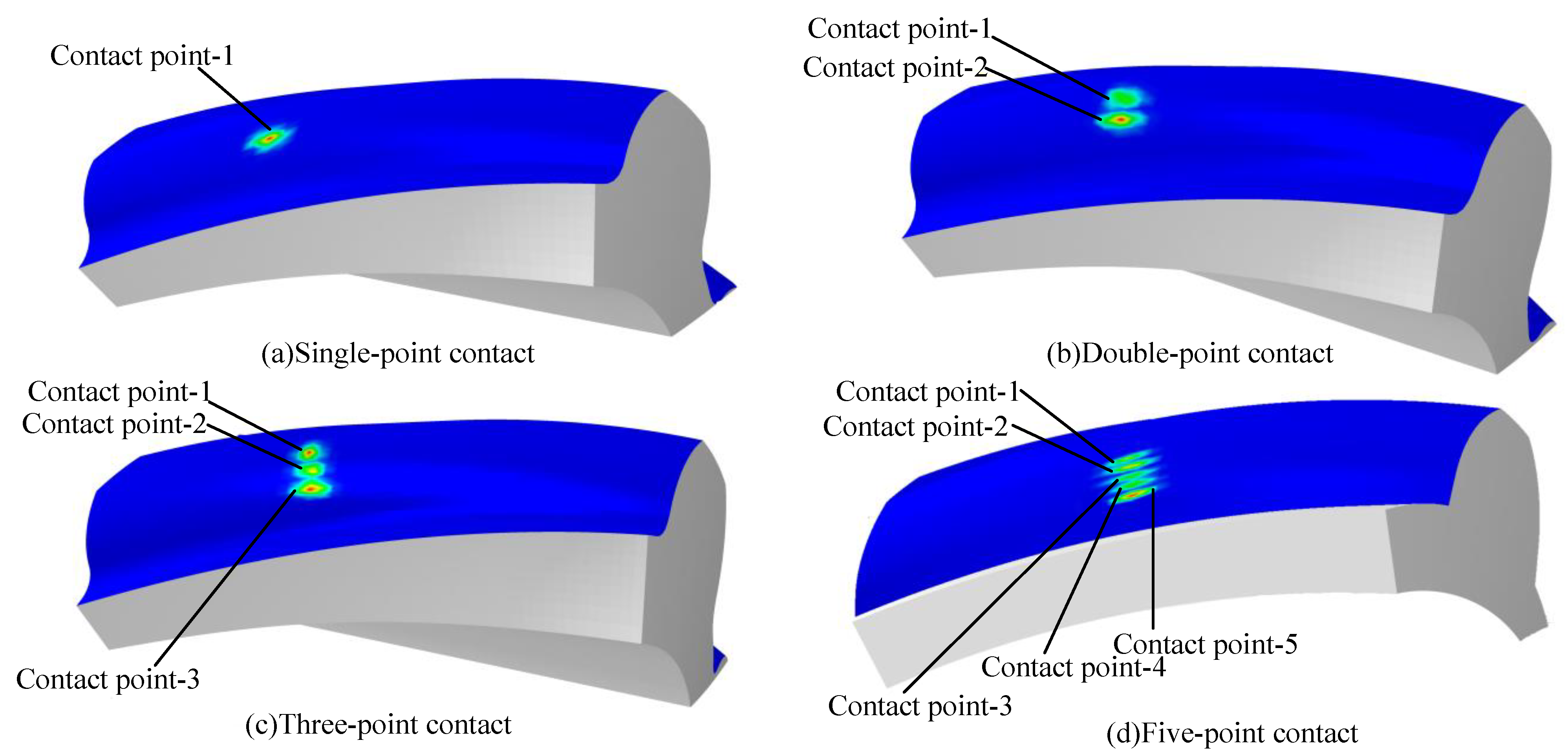
3.2. Design of Tooth Profile with Multi-Point Contact

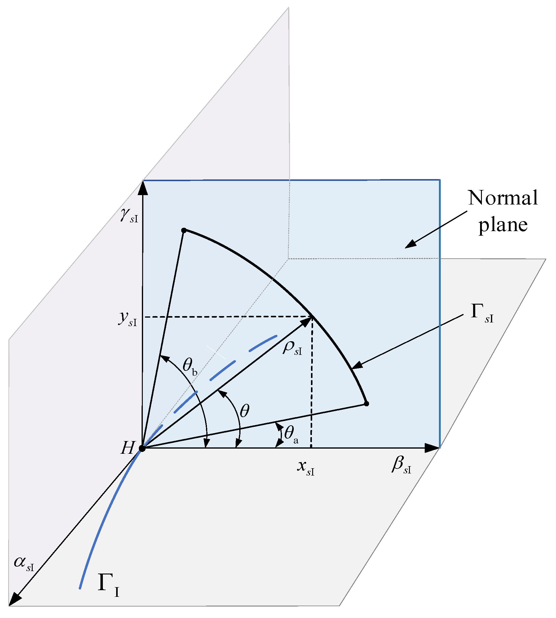
3.2.1. Tooth Profile Curve of Bevel Gear I

In accordance with the principles of tooth surface construction, the coordinate system S_fI is established at an arbitrary point H on spatial curve Γ_I by its tangent vector t_sI, principal normal vector m_sI, and binormal vector b_sI. Subsequently, within the normal plane formed by the principal normal vector m_sI and the binormal vector b_sI, an arc curve Γ_sI is constructed in the normal plane as the tooth profile curve of the bevel gear I, as shown in Figure 6. It should be noted that the principal normal vector m_sI should be consistent with n_I at the point H. The tooth profile curve of the bevel gear I in the normal plane is expressed [21]:

$${\Gamma }_{s\mathrm{I}}:\left\{\begin{array}{l}{x}_{s\mathrm{I}}={\rho }_{s\mathrm{I}}\cos \phi \\ y_{s\mathrm{I}}={\rho }_{s\mathrm{I}}\sin \phi \end{array}\right.$$

(15)

where, ρ_sI is the radius of arc curve Γ_sI at any point, φ is the angle between ρ_sI and m_sI, and the range of φ is: ${\phi }_{\mathrm{a}}\le \phi \le {\phi }_{\mathrm{b}}$.

3.2.2. Selection of Contact Points

N contact points are selected on the bevel gear I arc curve, as shown in Figure 7, and then the coordinates of the nth contact point A_n are:

$$A_n:\left\{\begin{array}{l}{x}_n={\rho }_{s\mathrm{I}}\cos {\phi }_n\\ y_n={\rho }_{s\mathrm{I}}\sin {\phi }_n\end{array}\right.(n=0,1,2,\cdots ,n)$$

(16)

3.2.3. Construction of Bevel Gear II Tooth Profile Curve

Considering that the tooth profile of bevel gear I is a segment of a circular curve and the selected contact point is on a circular curve, the tooth profile of bevel gear II is designed using the fitting method of the segmented quadratic trigonometric polynomial Bézier interpolation curves.

After determining the contact points, the adjacent contact points is connected with straight line in sequence and then edge vector a_u is obtained:

$$a_u=A_u-A_{u-1}(u=1,2,\cdots ,n)$$

(17)

Then, the tangent vector T_u of the interpolation curve to be constructed at point H_u is defined:

$$T_u=\left\{\begin{array}{l}{\tau }_u{a}_u+(1-{\tau }_u)a_{u+1}(u=1,2,\cdots ,n-1)\\ {\tau }_0{a}_1-(1-{\tau }_0)a_2(u=0)\\ {\tau }_n{a}_n-(1-{\tau }_n)a_{n-1}(u=n)\end{array}\right.$$

(18)

where, τ_u is the adjustment parameter of tangent vector, and the value range of τ_u is: 0 < τ_u < 1.

According to the definition of tangent vector T_u, by adjusting the tangent vector parameter t_u to make T_u and T_u+1 not parallel, so that the tangent line passing through point A_u with T_u as the tangent vector intersects with the tangent line passing through point A_u+1 with T_u+1 as the tangent vector, as shown in Figure 8. The intersection point V_u is denoted:

$$V_u=A_u+\frac{\left|a_{u+1}\times T_{u+1}\right|}{\left|T_u\times T_{u+1}\right|}{T}_u(u=0,1,\cdots ,n-1)$$

(19)

In the light of the contact point A_u and the intersection V_u of the tangent vectors, the four control points of the quadratic triangular Bézier curve l_u-II(ξ) passing through the point A_u-1 and the point A_u as follows:

$$\left\{\begin{array}{l}{p}_{u0}=A_{u-1}\\ p_{u1}={\eta }_u{A}_{u-1}+(1-{\eta }_u)V_{u-1}\\ p_{u2}={\chi }_u{A}_u+(1-{\chi }_u)V_{u-1}\\ p_{u3}=A_u\end{array}\right.(u=1,2,\cdots ,n)$$

(20)

where, η_u and χ_u are both adjustable parameters, the value range of them are respectively:

$$\left\{\begin{array}{l}0<{\eta }_u<1\\ 0<{\chi }_u<1\end{array}\right.$$

(21)

In accordance with the definition of quadratic triangular Bézier curve, l_u-II(ξ) is obtained:

$$l_{u\text{-II}}(\xi )=X_0(\xi )p_{u0}+X_1(\xi )p_{u1}+X_2(\xi )p_{u2}+X_3(\xi )p_{u3}$$

(22)

where, $X_0(\xi ),X_1(\xi ),X_2(\xi )$, and $X_3(\xi )$ are the primary function, they are defined:

$$\left\{\begin{array}{l}{X}_0(\xi )=(1-\sin \xi )(1-\lambda \sin \xi )\\ X_1(\xi )=(1-\sin \xi )(\sin \xi +\lambda \sin \xi )\\ X_2(\xi )=(1-\cos \xi )(\cos \xi +\lambda \cos \xi )\\ X_3(\xi )=(1-\cos \xi )(1-\lambda \cos \xi )\end{array}\right.$$

(23)

where, ξ is the variable, the range of ξ is: 0 ≤ ξ ≤ π/2, and λ is the parameter, the value range of λ is: $-1\le \lambda \le 1$.

3.3. Construction of Tooth Surface

3.3.1. Construction of Tooth Surface for Bevel Gear I

The section curve Γ_sI of bevel gear I in coordinate system S_fI is expressed:

$${\mathit{r}}_{sf\mathrm{I}}={\left(\begin{array}{cc}\begin{array}{ccc}{x}_{s\mathrm{I}}& y_{s\mathrm{I}}& 0\end{array}& 1\end{array}\right)}^T$$

(24)

Based on the principle of construction mentioned earlier, the constructed tooth surface Σ_I is obtained, and the Σ_I in coordinate system $S_{\mathrm{I}}$ is represented:

$${\mathit{r}}_{\mathrm{\Sigma }\mathrm{I}}(\phi ,t_{\mathrm{I}})={\mathit{M}}_{pf\mathrm{I}}{\mathit{r}}_{sf\mathrm{I}}$$

(25)

where,

$${\mathit{M}}_{pf\mathrm{I}}=\left(\begin{array}{cc}\begin{array}{ccc}{\mathit{i}}_{s\mathrm{I}}\cdot {\mathit{\beta }}_{s\mathrm{I}}& {\mathit{i}}_{s\mathrm{I}}\cdot {\mathit{\gamma }}_{s\mathrm{I}}& {\mathit{i}}_{s\mathrm{I}}\cdot {\mathit{\alpha }}_{s\mathrm{I}}\\ {\mathit{j}}_{s\mathrm{I}}\cdot {\mathit{\beta }}_{s\mathrm{I}}& {\mathit{j}}_{s\mathrm{I}}\cdot {\mathit{\gamma }}_{s\mathrm{I}}& {\mathit{j}}_{s\mathrm{I}}\cdot {\mathit{\alpha }}_{s\mathrm{I}}\\ {\mathit{k}}_{s\mathrm{I}}\cdot {\mathit{\beta }}_{s\mathrm{I}}& {\mathit{k}}_{s\mathrm{I}}\cdot {\mathit{\gamma }}_{s\mathrm{I}}& {\mathit{k}}_{s\mathrm{I}}\cdot {\mathit{\alpha }}_{s\mathrm{I}}\\ 0& 0& 0\end{array}& L_{\mathrm{I}}(t_{\mathrm{I}})\end{array}\right)$$

(26)

3.3.2. Construction of Tooth Surface for Bevel Gear II

According to the conjugate curve principle in the second section, the conjugate curve Γ_II of spatial curve Γ_I was obtained. Then, the coordinate system S_fII is established at an arbitrary point on conjugate curve Γ_II by its tangent vector α_II, principal normal vector β_II, and binormal vector γ_II. Unlike the section curve Γ_s1 of bevel gear I, the section curve Γ_s2 of bevel gear II is composed of a segment of interpolation curve l_u-II(ξ), and the interpolation curve l_u-II(ξ) in coordinate system S_fII is expressed:

$${\mathit{r}}_{sfu}^g={\left(\begin{array}{cc}\begin{array}{ccc}{x}_u^g& y_u^g& 0\end{array}& 1\end{array}\right)}^T$$

(27)

Therefore, the constructed tooth surface ${\mathrm{\Sigma }}_u^g$ is obtained, and the ${\mathrm{\Sigma }}_u^g$ in coordinate system S_II is represented:

$${\mathit{r}}_{\mathrm{\Sigma }u}^g={\mathit{M}}_{pf\mathrm{II}}{\mathit{r}}_{sfu}^g$$

(28)

where,

$${\mathit{M}}_{pf\mathrm{II}}=\left(\begin{array}{cc}\begin{array}{ccc}{\mathit{i}}_{s\mathrm{II}}\cdot {\mathit{\beta }}_{s\mathrm{II}}& {\mathit{i}}_{s\mathrm{II}}\cdot {\mathit{\gamma }}_{s\mathrm{II}}& {\mathit{i}}_{s\mathrm{II}}\cdot {\mathit{\alpha }}_{s\mathrm{II}}\\ {\mathit{j}}_{s\mathrm{II}}\cdot {\mathit{\beta }}_{s\mathrm{II}}& {\mathit{j}}_{s\mathrm{II}}\cdot {\mathit{\gamma }}_{s\mathrm{II}}& {\mathit{j}}_{s\mathrm{II}}\cdot {\mathit{\alpha }}_{s\mathrm{II}}\\ {\mathit{k}}_{s\mathrm{II}}\cdot {\mathit{\beta }}_{s\mathrm{II}}& {\mathit{k}}_{s\mathrm{II}}\cdot {\mathit{\gamma }}_{s\mathrm{II}}& {\mathit{k}}_{s\mathrm{II}}\cdot {\mathit{\alpha }}_{s\mathrm{II}}\\ 0& 0& 0\end{array}& L_{\mathrm{II}}(t_{\mathrm{II}})\end{array}\right)$$

(29)

4. Gear Tooth Characteristics Analysis

4.1. Continuity Conditions of Tooth Surface

When constructing tooth surfaces, it is essential to ensure the continuity of the tooth surface. According to the principles of tooth surface construction, it is known that when the tooth profile curve is continuous, the generated tooth surface is also continuous. Therefore, it is necessary to derive the continuity conditions of the tooth profile curve for bevel gear II. For interpolation curves, C² continuity is generally required, meaning that the second derivative of the curve is continuous [27,28,29]. In order to achieve smoother interpolation curves and a smoother surface formed by these curves, this paper derives the conditions for C³ continuity of the interpolation curves, ensuring that the third derivative of the interpolation curves is continuous [30].

The values of the interpolation curve l_u-II(ξ) at the starting point and endpoint of the u-th segment respectively are:

$$l_{u\text{-II}}(0)=p_{u0}$$

(30)

$$l_{u\text{-II}}(\frac{\pi }{2})=p_{u3}$$

(31)

The values of the interpolation curve l_u-II(ξ) at the starting point and endpoint of the (u + 1)-th segment respectively are:

$$l_{u+1\text{-}\mathrm{II}}(0)=p_{(u+1)0}$$

(32)

$$l_{u+1\text{-}\mathrm{II}}(\frac{\pi }{2})=p_{(u+1)3}$$

(33)

It can be concluded from Equation (26) that:

$$p_{u3}=p_{(u+1)0}=A_u$$

(34)

The first derivative of the interpolation curve l_u-II(ξ) is obtained:

$${l_{u\text{-}\mathrm{II}}}^{\prime }(\xi )=(1+\lambda )(p_{u1}-p_{u0})\cos \xi +\left(\left(p_{u3}-p_{u2}\right)\left(1+\lambda \right)+2\left(p_{u0}\lambda +(-p_{u1}+p_{u2})\left(1+\lambda \right)-p_{u3}\lambda \right)\cos \xi \right)\sin \xi$$

(35)

The second derivative of the interpolation curve l_u-II(ξ) is obtained:

$${l_{u\text{-}\mathrm{II}}}^{″}(\xi )=\left(p_{u3}-p_{u2}\right)\left(1+\lambda \right)\cos \xi +2\left((p_{u0}-p_{u3})\lambda +(p_{u2}-p_{u1})\left(1+\lambda \right)\right)\cos 2\xi +\left(p_{u0}-p_{u1}\right)\left(1+\lambda \right)\sin \xi$$

(36)

The third derivative of the interpolation curve l_u-II(ξ) is obtained:

$${l_{u\text{-}\mathrm{II}}}^{‴}(\xi )=\left(p_{u2}-p_{u3}\right)\left(1+\lambda \right)\sin \xi +\left(\left(p_{u0}-p_{u1}\right)\left(1+\lambda \right)+8\left(\left(p_{u3}-p_{u0}\right)\lambda +(p_{u1}-p_{u2})\left(1+\lambda \right)\right)\sin \xi \right)\cos \xi$$

(37)

To ensure the C¹ continuity of the interpolation curve l_u-II(ξ), the first derivative of the interpolation curve l_u-II(ξ) needs to be continuous, that is:

$${l_{u+1\text{-}\mathrm{II}}}^{\prime }(0)={l_{u\text{-}\mathrm{II}}}^{\prime }(\frac{\pi }{2})$$

(38)

According to Equation (20), the first derivatives of the interpolation curve at the starting-point and endpoint values can be obtained as follows:

$${l_{u+1\text{-}\mathrm{II}}}^{\prime }(0)=(1+{\lambda }_u)(p_{(u+1)1}-p_{(u+1)0})$$

(39)

$${l_{u\text{-}\mathrm{II}}}^{\prime }(\frac{\pi }{2})=(1+{\lambda }_{u+1})(p_{u3}-p_{u2})$$

(40)

Substituting Equations (34), (39) and (40) into (38), it could be obtained by:

$${\eta }_{u+1}=1-(1-{\chi }_u)\frac{\left|A_u{V}_{u-1}\right|}{\left|A_u{V}_u\right|}$$

(41)

To ensure the C² continuity of the interpolation curve l_u-II(ξ), the second derivative of the interpolation curve l_u-II(ξ) needs to be continuous, that is:

$${l_{u+1\text{-}\mathrm{II}}}^{″}(0)={l_{u\text{-}\mathrm{II}}}^{″}(\frac{\pi }{2})$$

(42)

$${l_{u+1\text{-}\mathrm{II}}}^{″}(0)=2{\lambda }_{u+1}{p}_{(u+1)0}-2(1+{\lambda }_{u+1})p_{(u+1)1}+(1+{\lambda }_{u+1})p_{(u+1)2}+(1-{\lambda }_{u+1})p_{(u+1)3}$$

(43)

$${l_{u\text{-}\mathrm{II}}}^{″}(\frac{\pi }{2})=(1-{\lambda }_u)p_{u0}+(1+{\lambda }_u)p_{u1}-2(1+{\lambda }_u)p_{u2}+2{\lambda }_u{p}_{u3}$$

(44)

Substituting Equation (34) into (42):

$${\lambda }_u={\lambda }_{u+1}$$

(45)

The range of values for λ_u is $0\le {\lambda }_u\le 1$, and in order to achieve the continuity of the interpolation curve l_u-II(ξ),

$${\lambda }_u={\lambda }_{u+1}=1$$

(46)

Substituting Equations (20), (43) and (44) into (42):

$$X_{u+1}=\frac{(3-4X_u)\left|V_{u-1}{A}_u\right|-{\eta }_u\left|A_{u-1}{V}_{u-1}\right|-\left|A_u{V}_u\right|}{\left|V_u{A}_{u+1}\right|}$$

(47)

Because the range of $X_u$ is $0<X_{u+1}<1$, it is deduced:

$$\frac{(3-4X_u)\left|V_{u-1}{A}_u\right|-\left|A_u{V}_u\right|-\left|V_u{A}_{u+1}\right|}{\left|V_{u-1}{A}_{u-1}\right|}<{\eta }_u<\frac{(3-4X_u)-\left|A_u{V}_u\right|}{\left|V_{u-1}{A}_{u-1}\right|}$$

(48)

The third derivative of the interpolation curve l_u-II(ξ) needs to be continuous, that is:

$${l_{u+1\text{-}\mathrm{II}}}^{‴}(0)=\left(p_{(u+1)0}-p_{(u+1)1}\right)\left(1+{\lambda }_{u+1}\right)$$

(49)

$${l_{u\text{-}\mathrm{II}}}^{‴}(\frac{\pi }{2})=\left(p_{u2}-p_{u3}\right)\left(1+{\lambda }_u\right)$$

(50)

According to Equation (42), it could be concluded that:

$$p_{(u+1)1}=2p_{u3}-p_{u2}$$

(51)

Substituting Equations (34) and (51) into (49):

$${l_{u+1\text{-}\mathrm{II}}}^{‴}(0)=\left(p_{u2}-p_{u3}\right)\left(1+{\lambda }_u\right)$$

(52)

Therefore, it could be deduced by:

$${l_{u+1\text{-}\mathrm{II}}}^{‴}(0)={l_{u\text{-}\mathrm{II}}}^{‴}(\frac{\pi }{2})$$

(53)

This implies that the interpolation curve satisfies C³ continuity, and when the interpolated curve satisfies C² continuity, the interpolated curve automatically satisfies C³ continuity. Consequently, when the interpolated curve satisfies Equations (34), (41), (47) and (48) then the interpolated curve l_u-II(ξ) can achieve C³ continuity.

4.2. Non-Interference Condition of Tooth Surface

The interpolation curve is constructed after satisfying the condition of C³ continuity, and then the tooth surface is constructed according to the construction principle. It is necessary to conduct interference analysis on the tooth surfaces of bevel gear I with multi-point contact and bevel gear II with multi-point contact and derive the condition that these two tooth surfaces do not interfere. According to the meshing theory of tooth surfaces, it could be determined whether there is curvature interference between two tooth surfaces based on the sign of the induced principal curvature.

If there is no curvature interference between these two tooth surfaces Σ_I and Σ_II, the induced normal curvature $K_1^{\text{I-II}}$ of tooth surfaces Σ_I and the induced normal curvature $K_2^{\text{I-II}}$ of tooth surfaces Σ_I are positive values. This is the condition where there is no interference between the contact points of the bevel gear teeth, expressed as:

$$\left\{\begin{array}{l}{K}_1^{\text{I-II}}>0\\ K_2^{\text{I-II}}>0\end{array}\right.$$

(54)

According to the principles of differential geometry and tooth profile construction, the principal curvatures $K_1^{\text{I-II}}$ and $K_2^{\text{I-II}}$ could be determined:

$$K_1^{\text{I-II}}=K_1^{\mathrm{I}}-K_1^{\mathrm{II}}$$

(55)

$$K_2^{\text{I-II}}=K_2^{\mathrm{I}}-K_2^{\mathrm{II}}$$

(56)

where, $K_1^{\mathrm{I}}$ and $K_1^{\mathrm{II}}$ are the two principal curvatures of tooth profile Σ_I; $K_2^{\mathrm{I}}$ and $K_2^{\mathrm{II}}$ are the two principal curvatures of tooth profile Σ_II.

According to differential geometry, $K_1^{\mathrm{I}}$ and $K_2^{\mathrm{I}}$ satisfy the equation:

$$\left(E^{\mathrm{I}}{G}^{\mathrm{I}}-{\left(F^{\mathrm{I}}\right)}^2\right){\left(K_{\kappa }^{\mathrm{I}}\right)}^2-\left(L^{\mathrm{I}}{G}^{\mathrm{I}}-2M^{\mathrm{I}}{F}^{\mathrm{I}}+N^{\mathrm{I}}{E}^{\mathrm{I}}\right)K_{\kappa }^{\mathrm{I}}+\left(L^{\mathrm{I}}{N}^{\mathrm{I}}-{\left(M^{\mathrm{I}}\right)}^2\right)=0$$

(57)

where, κ represents I or II, the first and second fundamental form coefficients E^I, F^I, G^I, L^I, M^I, N^I for tooth surface Σ_I can be separately derived [31]:

$$\left\{\begin{array}{l}{E}^{\mathrm{I}}=D(r_{\mathrm{\Sigma }\mathrm{I}}(\phi ,t_{\mathrm{I}}),\phi )D(r_{\mathrm{\Sigma }\mathrm{I}}(\phi ,t_{\mathrm{I}}),\phi )\\ F^{\mathrm{I}}=D(r_{\mathrm{\Sigma }\mathrm{I}}(\phi ,t_{\mathrm{I}}),\phi )D(r_{\mathrm{\Sigma }\mathrm{I}}(\phi ,t_{\mathrm{I}}),t_{\mathrm{I}})\\ G^{\mathrm{I}}=D(r_{\mathrm{\Sigma }\mathrm{I}}(\phi ,t_{\mathrm{I}}),t_{\mathrm{I}})D(r_{\mathrm{\Sigma }\mathrm{I}}(\phi ,t_{\mathrm{I}}),t_{\mathrm{I}})\\ L^{\mathrm{I}}=-D(r_{\mathrm{\Sigma }\mathrm{I}}(\phi ,t_{\mathrm{I}}),\phi )D(n_{\mathrm{\Sigma }\mathrm{I}}(\phi ,t_{\mathrm{I}}),\phi )\\ M^{\mathrm{I}}=-D(r_{\mathrm{\Sigma }\mathrm{I}}(\phi ,t_{\mathrm{I}}),\phi )D(n_{\mathrm{\Sigma }\mathrm{I}}(\phi ,t_{\mathrm{I}}),t_{\mathrm{I}})\\ N^{\mathrm{I}}=-D(r_{\mathrm{\Sigma }\mathrm{I}}(\phi ,t_{\mathrm{I}}),t_{\mathrm{I}})D(n_{\mathrm{\Sigma }\mathrm{I}}(\phi ,t_{\mathrm{I}}),t_{\mathrm{I}})\end{array}\right.$$

(58)

where, D(r_ΣI(φ,t_I),φ) is the first derivative of r_ΣI(φ,t_I) with respect to the parameter φ, and D(r_ΣI(φ,t_I),t_I) is the first derivative of r_ΣI(φ,t_I) with respect to the parameter t_I, D(n_ΣI(φ,t_I),φ) is the first derivative of unit normal vector n_ΣI(φ,t_I) of tooth surface r_ΣI with respect to the parameter φ, and D(n_ΣI(φ,t_I),t_I) is the first derivative of n_ΣI(φ,t_I) with respect to the parameter t_I.

The unit normal vector n_ΣI(φ,t_I) of tooth surface r_ΣI is obtained:

$$n_{\mathrm{\Sigma }\mathrm{I}}(\phi ,t_{\mathrm{I}})=\frac{D(r_{\mathrm{\Sigma }\mathrm{I}}(\phi ,t_{\mathrm{I}}),\phi )\times D(r_{\mathrm{\Sigma }\mathrm{I}}(\phi ,t_{\mathrm{I}}),t_{\mathrm{I}})}{\left|D(r_{\mathrm{\Sigma }\mathrm{I}}(\phi ,t_{\mathrm{I}}),\phi )\times D(r_{\mathrm{\Sigma }\mathrm{I}}(\phi ,t_{\mathrm{I}}),t_{\mathrm{I}})\right|}$$

(59)

For bevel gear II, it is necessary to determine the corresponding principal curvatures $K_1^{\text{I-II}}$ and $K_2^{\text{I-II}}$ of the tooth surface $r_{\mathrm{\Sigma }u}^g$ formed by the interpolation curves l_u-II(ξ) in different segments.

According to differential geometry, $K_1^{\mathrm{II}}$ and $K_2^{\mathrm{II}}$ satisfy the equation:

$$\left(E^{\mathrm{II}}{G}^{\mathrm{II}}-{\left(F^{\mathrm{II}}\right)}^2\right){\left(K_{\kappa }^{\mathrm{II}}\right)}^2-\left(L^{\mathrm{II}}{G}^{\mathrm{II}}-2M^{\mathrm{II}}{F}^{\mathrm{II}}+N^{\mathrm{II}}{E}^{\mathrm{II}}\right)K_{\kappa }^{\mathrm{II}}+\left(L^{\mathrm{II}}{N}^{\mathrm{II}}-{\left(M^{\mathrm{II}}\right)}^2\right)=0$$

(60)

where, the first and second fundamental form coefficients E^II, F^II, G^II, L^II, M^II, N^II for tooth surface ${\mathrm{\Sigma }}_{\mathrm{II}}$ can be separately derived [31]:

$$\left\{\begin{array}{l}{E}^{\mathrm{II}}=D(r_{\mathrm{\Sigma }u}^g(\xi ,t_{\mathrm{II}}),\xi )D(r_{\mathrm{\Sigma }u}^g(\xi ,t_{\mathrm{II}}),\xi )\\ F^{\mathrm{II}}=D(r_{\mathrm{\Sigma }u}^g(\xi ,t_{\mathrm{II}}),\xi )D(r_{\mathrm{\Sigma }u}^g(\xi ,t_{\mathrm{II}}),t_{\mathrm{II}})\\ G^{\mathrm{II}}=D(r_{\mathrm{\Sigma }u}^g(\xi ,t_{\mathrm{II}}),t_{\mathrm{II}})D(r_{\mathrm{\Sigma }u}^g(\xi ,t_{\mathrm{II}}),t_{\mathrm{II}})\\ L^{\mathrm{II}}=-D(r_{\mathrm{\Sigma }u}^g(\xi ,t_{\mathrm{II}}),\xi )D(n_{\mathrm{\Sigma }u}^g(\xi ,t_{\mathrm{II}}),\xi )\\ M^{\mathrm{II}}=-D(r_{\mathrm{\Sigma }u}^g(\xi ,t_{\mathrm{II}}),\xi )D(n_{\mathrm{\Sigma }u}^g(\xi ,t_{\mathrm{II}}),t_{\mathrm{II}})\\ N^{\mathrm{II}}=-D(r_{\mathrm{\Sigma }u}^g(\xi ,t_{\mathrm{II}}),t_{\mathrm{II}})D(n_{\mathrm{\Sigma }u}^g(\xi ,t_{\mathrm{II}}),t_{\mathrm{II}})\end{array}\right.$$

(61)

where, $D(r_{\mathrm{\Sigma }u}^g(\xi ,t_{\mathrm{II}}),\xi )$ is the first derivative of $r_{\mathrm{\Sigma }u}^g(\xi ,t_{\mathrm{II}})$ with respect to the parameter $\xi$, and $D(r_{\mathrm{\Sigma }u}^g(\xi ,t_{\mathrm{II}}),t_{\mathrm{II}})$ is the first derivative of $r_{\mathrm{\Sigma }u}^g(\xi ,t_{\mathrm{II}})$ with respect to the parameter $t_{\mathrm{II}}$, $D(n_{\mathrm{\Sigma }u}^g(\xi ,t_{\mathrm{II}}),\xi )$ is the first derivative of unit normal vector $n_{\mathrm{\Sigma }u}^g(\xi ,t_{\mathrm{II}})$ of tooth surface $r_{\mathrm{\Sigma }u}^g$ with respect to the parameter $\xi$, and $D(n_{\mathrm{\Sigma }u}^g(\xi ,t_{\mathrm{II}}),t_{\mathrm{II}})$ is the first derivative of $n_{\mathrm{\Sigma }u}^g(\xi ,t_{\mathrm{II}})$ with respect to the parameter $t_{\mathrm{II}}$.

5. Analysis of Load-Bearing Characteristics

5.1. Bevel Gear Pair Parameters

According to the principles outlined in Section 2 and Section 3, tooth surfaces with single-point, two-point, three-point, and five-point contact based on the fundamental parameters in

Table 1. Basic parameters of bevel gear pairs.

Parameter	Bevel Gear I	Bevel Gear II
Number of teeth	8	24
Module	6.75 mm
Pitch cone angle	18.435 deg.	71.565 deg.
Spiral angle	35 deg.
Hand of spiral	Left hand	Right hand
Shaft angle	90 deg.
Face width	30 mm
Outer cone distance	83.48 mm	250.45 mm

are constructed. Subsequently, the complete gear pairs were assembled. Figure 9 shows the model of a bevel gear pair with five-point contact.

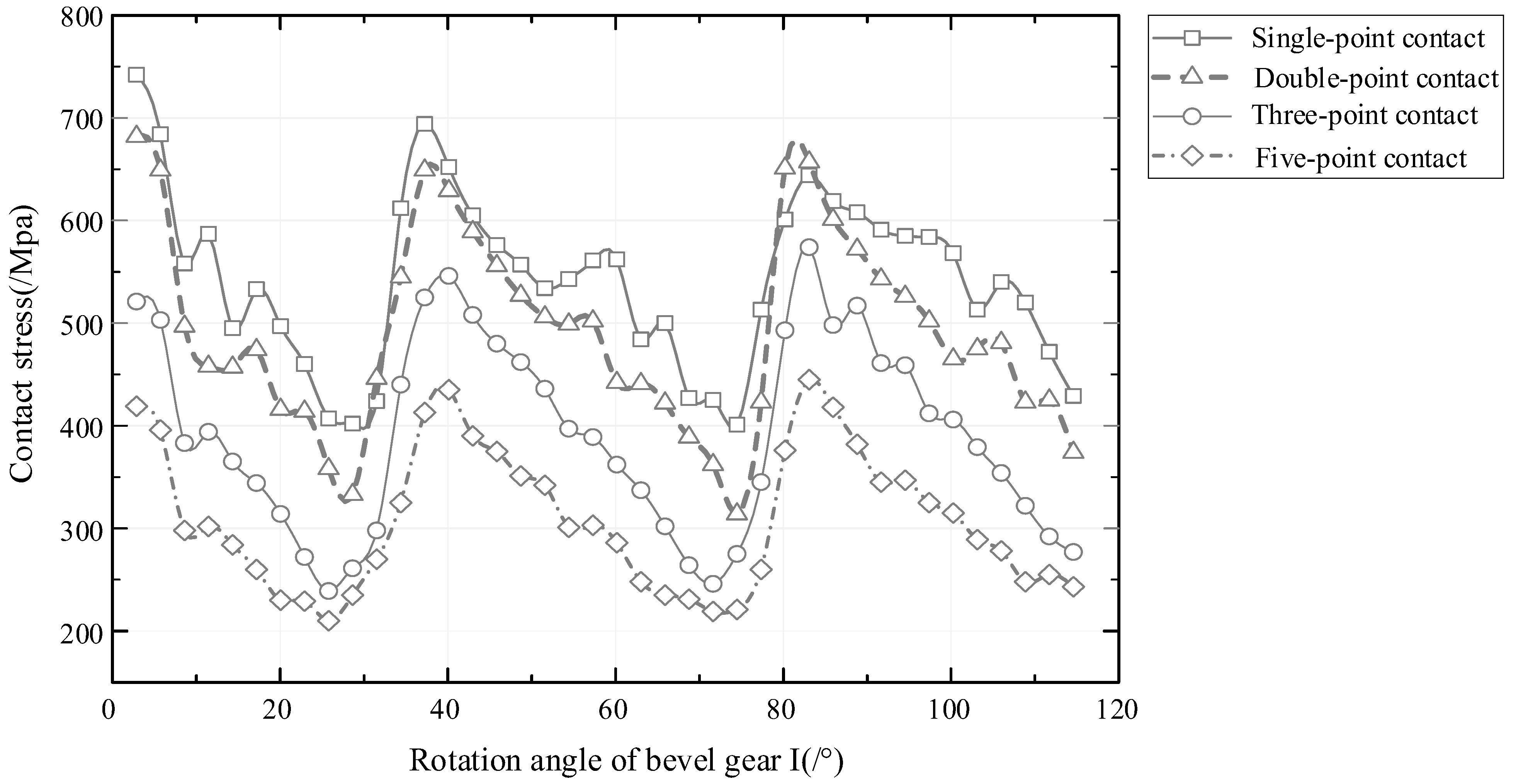
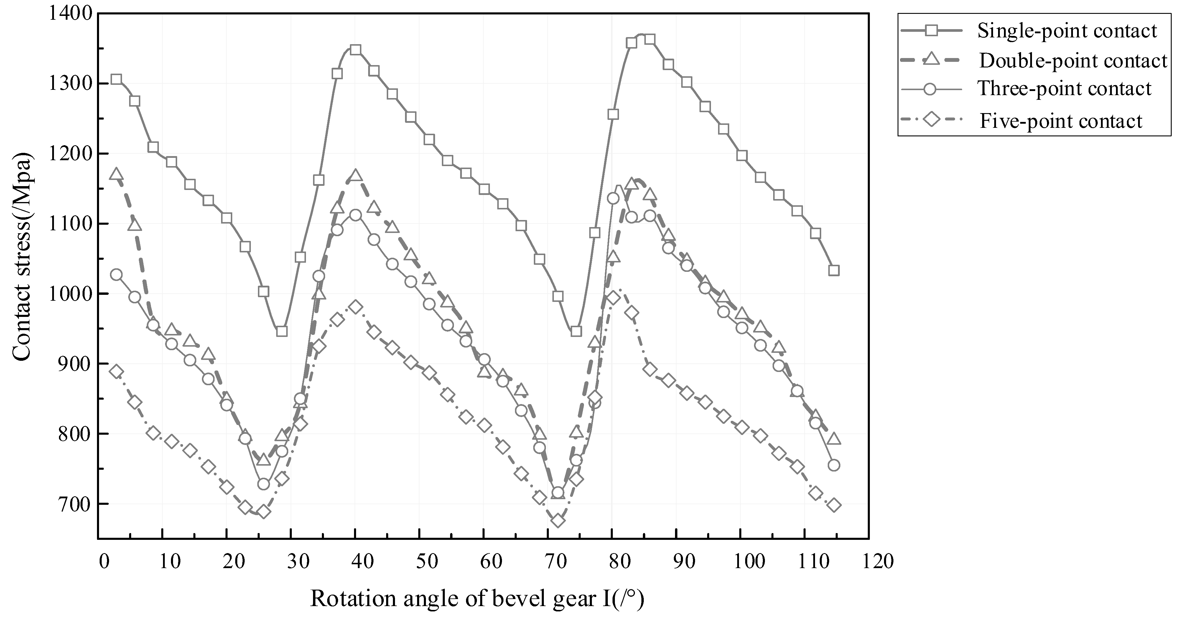
5.2. Influence of Meshing Points on Contact Stress

According to the established models of bevel gear pairs with single-point, two-point, three-point, and five-point contact, contact simulations were conducted using the Abaqus software. When partitioning the mesh, C3D8I elements were employed, yielding a mesh size of approximately 0.35. The total number of mesh elements amounted to 422,400 [24]. When selecting materials, structural steel was chosen with an elastic modulus set to 210 GPa, the Poisson’s ratio is set to 0.3 and the yield strength is 850 MPa, the fracture strength is 1200 MPa [22], and the boundary conditions are set as shown in Figure 10. In Figure 10, bevel gear I and bevel gear II each have only one degree of freedom for rotation around their respective axes. An angular velocity of 3.5 rad/s around the z_I axis is applied to bevel gear I, the torque of 100 Nm and 540 Nm are applied to the bevel gear II to resist the rotation of bevel gear I, respectively.

The established models of bevel gears with single-point, double-point, triple-point, and five-point contacts obtained contact pattern through simulation experiments, as shown in Figure 11. It is evident in Figure 11 that the distribution of contact points varies along the tooth height direction. The contact pattern for a single-point contact bevel gear is an ellipse close to the middle position of the tooth. For the bevel gear with double-point contact, the contact pattern consists of two ellipses. Similarly, the bevel gear with three-point contact has three ellipses, and the bevel gear with five-point contact has five ellipses. The ellipses are distributed along the tooth height direction, with the long axis in the tooth width direction. This is consistent with the contact trajectory of the literature [25,26], where there is full-width contact along the tooth width direction, and there are multiple contact points in the tooth height direction. As the bevel gear pair moves, the contact ellipses move along the tooth width direction, achieving full-width contact, as shown in Figure 12.

When the load torque of 100 Nm and 540 Nm are applied in the bevel gear II, the range from 0 degree to 22 degrees is the single tooth meshing area, the range from 22 degrees to 36 degrees is the double tooth meshing area. Subsequently, when the bevel gear I rotates from 36 degrees to 68 degrees, it corresponds to the first complete single-tooth engagement region. By repeating this process, the contact stress variation law of the bevel gear pair with multi-point contact based on the geometric elements could be obtained, as shown in Figure 13 and Figure 14. When the number of meshing teeth is the same, the contact stress on the small gear decreases gradually from the small end to the large end. The maximum contact stress occurs on the bevel gear with single-point contact, followed by the bevel gear with double-point contact. Then the contact stress on the bevel gear with three-point contact is smaller than that on the bevel gear with double-point contact, and the lowest contact stress is observed on the bevel gear with five-point contact. Multi-point contact for bevel gear based on the geometric elements can effectively decrease the contact stress, this is consistent with the results in the literature [26].

When the load applied in the bevel gear II is 100 Nm, the maximum contact stress on the bevel gear with single point contact in the first complete single-tooth engagement region is 742 MPa, it is 682 MPa for the bevel gear with double-point contact, it is 546 MPa for the bevel gear with three-point contact, and it is 435 MPa for the bevel gear with five-point contact. The maximum contact stress for the bevel gear with five-point contact is reduced by 41.37% compared to the maximum contact stress of the bevel gear with single-point contact, by 36.22% compared to the maximum contact stress of the bevel gear with double-point contact, and by 20.33% compared to the maximum contact stress of the bevel gear with three-point contact.

When the load applied in the bevel gear II is 540 Nm, the maximum contact stress on the bevel gear with single point contact in the first complete single-tooth engagement region is 1348 MPa. This value is close to the maximum contact pressure value reported in the literature [32]. In the literature [32], when the torque of 600 Nm is applied to bevel gear II, the maximum contact pressure for single-point contact on the mating bevel gear is 1400 MPa. The maximum contact stress is 1169 MPa for the bevel gear with double-point contact, the maximum contact stress is 1112 MPa for the bevel gear with three-point contact, and the maximum contact stress is 981 MPa for the bevel gear with five-point contact. The maximum contact stress for the bevel gear with five-point contact is reduced by 27.23% compared to the maximum contact stress of the bevel gear with single-point contact, by 16.08% compared to the maximum contact stress of the bevel gear with double-point contact, and by 11.78% compared to the maximum contact stress of the bevel gear with three-point contact.

5.3. Influence of Distance between Contact Points on Contact Stress

Taking the example of double-point contact bevel gear pair, the influence of the distance between contact points on the contact stress of bevel gear pairs when the number of contact points is the same is analyzed. Models of bevel gear pairs with distances of 0.005 mm, 0.007 mm, and 0.01 mm between the double contact points are respectively is established for contact analysis. The resulting contact patterns are shown in Figure 15, double contact ellipses are depicted on the tooth surface, with these two contact ellipses distributed along the tooth height direction. The difference lies in that in diagram (c), the distance between the two contact ellipses is the greatest; in diagram (b), the distance between the two contact ellipses is next; and in diagram (a), the distance between the two contact ellipses is the smallest. As the distance between the contact points decreases, the distance between the two ellipses also decreases.

Figure 16 and Figure 17 depict the variation trend of contact stress for bevel gears based on geometric elements with double-point contact from engagement to disengagement under the load of 100 Nm and 540 Nm, respectively. From Figure 16 and Figure 17, it could be observed that the smaller the maximum non-contact distance between contact points, the lower the contact stress for the bevel gear based on geometric elements with the same number of contact points. A smaller maximum non-contact distance between contact points corresponds to lower contact stress and tends to approach contact along the tooth height line.

When the load applied in the bevel gear II is 100 Nm, the maximum contact stress on the bevel gear with the distance of 0.01 mm between the double contact points in the first complete single-tooth engagement region is 705 MPa, it is 682 MPa for the bevel gear with the distance of 0.007 mm between the double contact points, it is 542 MPa for the bevel gear with the distance of 0.005 mm between the double contact points. The maximum contact stress for the bevel gear with the distance of 0.005 mm between the double contact points is reduced by 23.21% compared to the maximum contact stress of the bevel gear with the distance of 0.007 mm between the double contact points, by 20.52% compared to the maximum contact stress of the bevel gear with the distance of 0.01 mm between the double contact points.

When the load applied in the bevel gear II is 540 Nm, the maximum contact stress on the bevel gear with the distance of 0.01 mm between the double contact points in the first complete single-tooth engagement region is 1328 MPa, it is 1169 MPa for the bevel gear with the distance of 0.007 mm between the double contact points, it is 1096 MPa for the bevel gear with the distance of 0.005 mm between the double contact points. The maximum contact stress for the bevel gear with the distance of 0.005 mm between the double contact points is reduced by 17.47% compared to the maximum contact stress of the bevel gear with the distance of 0.007 mm between the double contact points, by 6.24% compared to the maximum contact stress of the bevel gear with the distance of 0.01 mm between the double contact points.

6. Conclusions

In this paper, the design method of novel bevel gear with high load-capacity based on geometric elements have been proposed, and then the correlation analysis and experimental verification of the novel bevel gear were carried out. Throughout the research, there are several conclusions as follows:

(1)

The design method of bevel gear with high load-capacity is put forward, the proposed novel gear enables multi-point contact in the tooth height direction, and full-tooth-width contact along the tooth width direction.

(2)

The mathematical model of novel bevel gear is established, and then the analysis of gear tooth characteristics is conducted, conditions for tooth surface continuity and non-interference are also deduced.

(3)

The load-bearing characteristics are analyzed, revealing that increasing the number of contact points can reduce the contact stress. For the bevel gear pair with five-point contact, the contact stress is 41.37% lower than that of a bevel gear pair with single-point contact under the torque of 100 Nm.

(4)

When the number of contact points is the same, increasing the distance between the contact points can also reduce the contact stress.

(5)

For the bevel gear pairs with multi-point contact based on the geometric elements, it requires higher tooth surface accuracy and still face challenges in manufacturing, which need to be further addressed.

References

1. Klingelnberg, J. (Ed.) Fields of Application for Bevel Gears. In Bevel Gear: Fundamentals and Applications; Springer: Berlin/Heidelberg, Germany, 2016; pp. 1–10. [Google Scholar]
2. Zhou, C.J.; Li, Z.D.; Hu, B.; Zhan, H.F.; Han, X. Analytical solution to bending and contact strength of spiral bevel gears in consideration of friction. Int. J. Mech. Sci. 2017, 128, 475–485. [Google Scholar] [CrossRef]
3. Jedlinski, L.; Jonak, J. A disassembly-free method for evaluation of spiral bevel gear assembly. Mech. Syst. Signal Process. 2017, 88, 399–412. [Google Scholar] [CrossRef]
4. Ding, H.; Tang, J.Y.; Zhong, J.; Zhou, Z.Y. A hybrid modification approach of machine-tool setting considering high tooth contact performance in spiral bevel and hypoid gears. J. Manuf. Syst. 2016, 41, 228–238. [Google Scholar] [CrossRef]
5. Yavuz, S.D.; Saribay, Z.B.; Cigeroglu, E. Nonlinear time-varying dynamic analysis of a spiral bevel geared system. Nonlinear Dyn. 2018, 92, 1901–1919. [Google Scholar] [CrossRef]
6. Kong, X.; Ding, H.; Huang, R.; Tang, J.Y. Adaptive data-driven modeling, prediction and optimal control for loaded transmission error of helicopter zero spiral bevel gear transmission system. Mech. Mach. Theory 2021, 165, 104417. [Google Scholar] [CrossRef]
7. Li, H.N.; Tang, J.Y.; Chen, S.Y.; Rong, K.B.; Ding, H.; Lu, R. Loaded contact pressure distribution prediction for spiral bevel gear. Int. J. Mech. Sci. 2023, 242, 108027. [Google Scholar] [CrossRef]
8. Mu, Y.M.; He, X.M. Design and dynamic performance analysis of high-contact-ratio spiral bevel gear based on the higher-order tooth surface modification. Mech. Mach. Theory 2021, 161, 104312. [Google Scholar] [CrossRef]
9. Song, B.Y.; Chen, J.; Zhou, Z.Y.; Rong, K.B.; Zhao, J.Y.; Ding, H. Sensitive misalignment oriented loaded contact pressure regulation model for spiral bevel gears. Mech. Mach. Theory 2023, 188, 105410. [Google Scholar] [CrossRef]
10. Vivet, M.; Tamarozzi, T.; Desmet, W.; Mundo, D. On the modelling of gear alignment errors in the tooth contact analysis of spiral bevel gears. Mech. Mach. Theory 2021, 155, 104065. [Google Scholar] [CrossRef]
11. Pigé, A.; Velex, P.; Lanquetin, R.; Cutuli, P. A model for the quasi-static and dynamic simulations of bevel gears. Mech. Mach. Theory 2022, 175, 104971. [Google Scholar]
12. Batsch, M. Mathematical model and tooth contact analysis of convexo-concave helical bevel Novikov gear mesh. Mech. Mach. Theory 2020, 149, 103842. [Google Scholar] [CrossRef]
13. Han, Q.K.; Chu, F.L. Nonlinear dynamic model for skidding behavior of angular contact ball bearings. J. Sound Vib. 2015, 354, 219–235. [Google Scholar] [CrossRef]
14. Chen, R.; Zhao, B.; He, T.; Tu, L.Y.; Xie, Z.L.; Zhong, N.; Zou, D.Q. Study on coupling transient mixed lubrication and time-varying wear of main bearing in actual operation of low-speed diesel engine. Tribol. Int. 2024, 191, 109159. [Google Scholar] [CrossRef]
15. Shi, J.H.; Zhao, B.; Tu, L.Y.; Xin, Q.; Xie, Z.L.; Zhong, N.; Lu, X.Q. Transient lubrication analysis of journal-thrust coupled bearing considering time-varying loads and thermal-pressure coupled effect. Tribol. Int. 2024, 194, 109502. [Google Scholar] [CrossRef]
16. Litvin, F.L.; Tsung, W.J.; Coy, J.J.; Heine, C. Method for generation of spiral bevel gears with conjugate gear tooth surfaces. J. Mech. Transm. Autom. Des. Trans. Asme 1987, 109, 163–170. [Google Scholar] [CrossRef]
17. Litvin, F.L.; Wang, A.G.; Handschuh, R.F. Computerized design and analysis of face-milled, uniform tooth height spiral bevel gear drives. J. Mech. Des. 1996, 118, 573–579. [Google Scholar] [CrossRef]
18. Litvin, F.L.; Fuentes, A.; Fan, Q.; Handschuh, R.F. Computerized design, simulation of meshing, and contact and stress analysis of face-milled formate generated spiral bevel gears. Mech. Mach. Theory 2002, 37, 441–459. [Google Scholar] [CrossRef]
19. Litvin, F.L.; Fuentes, A.; Hayasaka, K. Design, manufacture, stress analysis, and experimental tests of low-noise high endurance spiral bevel gears. Mech. Mach. Theory 2006, 41, 83–118. [Google Scholar] [CrossRef]
20. Chen, B.K.; Liang, D.; Li, Z.Y. A study on geometry design of spiral bevel gears based on conjugate curves. Int. J. Precis. Eng. Manuf. 2014, 15, 477–482. [Google Scholar] [CrossRef]
21. Peng, S.; Chen, B.K.; Liang, D.; Zhang, L.; Qin, S. Mathematical model and tooth contact analysis of an internal helical gear pair with selectable contact path. Int. J. Precis. Eng. Manuf. 2018, 19, 837–848. [Google Scholar] [CrossRef]
22. An, L.Q.; Zhang, L.H.; Qin, S.L.; Lan, G.; Chen, B.K. Mathematical design and computerized analysis of spiral bevel gears based on geometric elements. Mech. Mach. Theory 2021, 156, 104131. [Google Scholar] [CrossRef]
23. Tan, R.L.; Zhang, W.Q.; Guo, X.D.; Chen, B.K.; Shu, R.Z. An analytical framework of the kinematic geometry for general point-contact gears from contact path. Proc. Inst. Mech. Eng. Part C J. Mech. Eng. Sci. 2022, 236, 6363–6382. [Google Scholar] [CrossRef]
24. Tan, R.L.; Chen, B.K.; Xiang, D.; Liang, D. A study on the design and performance of epicycloid bevels of pure-rolling contact. ASME J. Mech. 2018, 140, 043301. [Google Scholar] [CrossRef]
25. Liang, D.; Li, M.; Jiang, P.; Meng, S. Optimization design and analysis of internal gear transmission with double contact points. Proc. Inst. Mech. Eng. Part C J. Mech. Eng. Sci. 2023, 237, 5788–5798. [Google Scholar] [CrossRef]
26. Liang, D.; Meng, S.; Gao, Y. Design principle and meshing analysis of internal gear drive with three contact points. Adv. Mech. Eng. 2022, 14, 16878132221081576. [Google Scholar] [CrossRef]
27. Li, J.; Song, L.; Liu, C. The cubic trigonometric automatic interpolation spline. IEEE/CAA J. Autom. Sin. 2018, 5, 1136–1141. [Google Scholar] [CrossRef]
28. Luo, Z.X. C1, C2-smooth interpolants on curved sides element. Comput. Math. Appl. 1998, 35, 125–130. [Google Scholar] [CrossRef]
29. Phung, V.M.; Nguyen, V.M.; Phan, T.H. Hermite interpolation on algebraic curves in C2. Indag. Math. 2019, 30, 874–890. [Google Scholar] [CrossRef]
30. Zhu, X.Y.; Wu, X.Q.; Chen, F.L. C~3 continuous shape-preserving piecewise quadratic triangular Bézier interpolation curves. J. Hunan Univ. Technol. 2012, 25, 25–29. [Google Scholar]
31. Chen, S.Y.; Zhang, A.Q.; Wei, J.; Lim, T.C. Nonlinear excitation and mesh characteristics model for spiral bevel gears. Int. J. Mech. Sci. 2023, 257, 108541. [Google Scholar] [CrossRef]
32. Tan, R.; Chen, B.K.; Peng, C.Y. General mathematical model of spiral bevel gears of continuous pure-rolling contact. Proc. Inst. Mech. Eng. Part C J. Mech. Eng. Sci. 2015, 229, 2810–2826. [Google Scholar] [CrossRef]
Figure 1. Schematic diagram of the novel bevel gear.
Mathematics 12 01373 g001
Figure 2. Conjugate curves.
Mathematics 12 01373 g002
Figure 3. Coordinate systems.
Mathematics 12 01373 g003
Figure 4. Schematic diagram of arbitrary normal vector.
Mathematics 12 01373 g004
Figure 5. Schematic diagram of tooth surface construction.
Mathematics 12 01373 g005
Figure 6. Tooth profile diagram of bevel gear I.
Mathematics 12 01373 g006
Figure 7. Selection of contact points.
Mathematics 12 01373 g007
Figure 8. Schematic diagram of intersection point Vu.
Mathematics 12 01373 g008
Figure 9. Bevel gear pairs with five-point contact.
Mathematics 12 01373 g009
Figure 10. Boundary condition.
Mathematics 12 01373 g010
Figure 11. Contact pattern of bevel gear with multi-point contact.
Mathematics 12 01373 g011
Figure 12. Diagram of full tooth width contact.
Mathematics 12 01373 g012
Figure 13. Contact stress of bevel gear pairs when loaded with 100 Nm load.
Mathematics 12 01373 g013
Figure 14. Contact stress of bevel gear pairs when loaded with 540 Nm load.
Mathematics 12 01373 g014
Figure 15. Contact patterns for bevel gears with different distances between contact points.
Mathematics 12 01373 g015
Figure 16. Contact stress of bevel gear pairs with double-point contact when loaded with 100 Nm load.
Mathematics 12 01373 g016
Figure 17. Contact stress of bevel gear pairs with double-point contact when loaded with 540 Nm load.
Mathematics 12 01373 g017