Lean-and-Green Strength Performance Optimization of a Tube-to-Tubesheet Joint for a Shell-and-Tube Heat Exchanger Using Taguchi Methods and Random Forests

Abstract

The failing tube-to-tubesheet joint is identified as a primary quality defect in the fabrication of a shell-and-tube heat exchanger. Operating in conditions of high pressure and temperature, a shell-and-tube heat exchanger may be susceptible to leakage around faulty joints. Owing to the ongoing low performance of the adjacent tube-to-tubesheet expansion, the heat exchanger eventually experiences malfunction. A quality improvement study on the assembly process is necessary in order to delve into the tight-fitting of the tube-to-tubesheet joint. We present a non-linear screening and optimization study of the tight-fitting process of P215NL (EN 10216-4) tube samples on P265GH (EN 10028-2) tubesheet specimens. A saturated fractional factorial scheme was implemented to screen and optimize the tube-to-tubesheet expanded-joint performance by examining the four controlling factors: (1) the clearance, (2) the number of grooves, (3) the groove depth, and (4) the tube wall thickness reduction. The adopted ‘green’ experimental tactic required duplicated tube-push-out test trials to form the ‘lean’ joint strength response dataset. Analysis of variance (ANOVA) and regression analysis were subsequently employed in implementing the Taguchi approach to accomplish the multifactorial non-linear screening classification and the optimal setting adjustment of the four investigated controlling factors. It was found that the tube-wall thickness reduction had the highest influence on joint strength (55.17%) and was followed in the screening hierarchy by the number of grooves (at 30.47%). The groove depth (at 7.20%) and the clearance (at 6.84%) were rather weaker contributors, in spite of being evaluated to be statistically significant. A confirmation run showed that the optimal joint strength prediction was adequately estimated. Besides exploring the factorial hierarchy with statistical methods, an algorithmic (Random Forest) approach agreed with the leading effects line-up (the tube wall thickness and the number of grooves) and offered an improved overall prediction for the confirmation-run test dataset.

1. Introduction

The shell-and-tube heat exchanger is a popular type of heat transfer equipment that is fabricated to efficiently remove heat from a higher-temperature medium and direct it toward a lower-temperature medium [1,2]. The heat flow is conducted through a solid separation, such that the two media are prevented from coming in direct contact and physically interacting [3]. It is well known that the shell-and-tube heat exchanger is a preferred equipment option in unit operations, by as much as 35–40% in industrial applications, due to some favorable aspects: (1) its production simplicity, (2) its production cost-effectiveness, (3) its convenient maintenance, and (4) its versatility in wide operating conditions [4,5,6,7].

The primary heat-exchanger failure mode is related to the tube-to-tubesheet joint connection performance [8,9,10,11,12,13,14,15]. A faulty joint may induce leakage incidents to a functioning heat exchanger. The strength and reliability of the tube-to-tubesheet joints heavily depend on the geometry of their components, their fabrication process, and their operating conditions [16,17,18,19]. The persisting issue of controlling the expansion pressure and operating temperature differentials on the connection capacity of hydraulically expanded joints still remains a puzzle in heat-exchanger fabrication [20,21,22,23]. The basic techniques for tube expansion are: (1) rolling, (2) explosive forming, and (3) hydraulic forming. Rolling is the most frequent tube-expansion process. The elevated rolling torques contribute to the over-thinning of the tube wall and they negatively affect the tube-tubesheet joint strength. The safe operation of a shell-and-tube heat exchanger is also impacted by the specification limits of the initial clearance to which tubesheet holes can be enlarged [24,25]. Ostensibly, the safety of the tube-to-tubesheet joints hinges upon the holding power and hydraulic tightness of the expanded tube joints and they should be experimentally determined. The joint integrity should be based on the relationship between the applied stress and its resulting deformation [26]. It is the axial strength and tightness that provide the quality indicators to measure the performance of the joints. In other words, to assess the extent of the mechanical failure, the tube-to-tubesheet joint integrity is measured by the limiting axial force. On the other hand, the effect of the geometry of the grooves is of paramount importance in the much broader cases that involve not only hydraulically expanded tube-to-tubesheet joints, but also welded, expanded and welded-expanded tube-to-tubesheet joints [27,28,29]. The effect of the grooves on the distribution of the residual contact pressure, between the outer surface of the tube and the inner surface of the tubesheet hole, is also related to the selected fabrication materials. The topology and configuration of the grooves are staple controlling factors in any pragmatic study that investigates the propensities of the joints. The push-out force is the designated quality characteristic response which will be examined in this study since it has a direct positive correlation with respect to the expansion pressure. From a production perspective, the tube expansion process for joining the tube ends with the tubesheet holes remains, even today, a time-consuming and costly process. Considering the various types of shell-and-tube heat exchangers, the number of tubes, which are needed to be tight-fitted to the available tubesheet area, range from an order of a hundred up to a thousand tubes; the volume of work for a single heat-exchanger unit grows fast to become profuse. It poses a production problem, because the fitting process is still manually executed. Meanwhile, the level of quality and cost-effectiveness should be such that to ensure that all the tube-to-tubesheet expanded joints meet the fail-safe operation condition. Of course, there is always the option to resort to the additional process step of welding the joints which entails a cogent action of assurance for a reliable unit functionality [30]. However, the welding process adds extra cost to the production of a heat-exchanger unit, besides elongating the assembly lead time. Under current manufacturing practices, the extra step of welding might not even be valued as a ‘lean’ activity.

Obviously, a lot of work has been carried out in the past on studying scientifically the tube-to-tubesheet expanded joints with the objective to increase manufacturing knowledge for making more robust and more reliable heat-exchanger products. This effort will take a different perspective by researching the performance improvement of the joints as it may be directly experienced on the production floor. Therefore, the first requirement is that experiments should be executed in the area that is affected the most, i.e., in the assembly room. Consequently, an empirical study will be organized in such a way that takes into account the same realistic restrictions, which are also applied to the traditional shop-floor investigations: (1) low-volume experimentation, (2) low-cost trial logistics, (3) minimal on-line processor interruptions, and (4) quick-turnaround data analysis. Actually, the seemingly stated restrictions may not be viewed as imposed procedural requirements, but normal guides for executing a modern lean engineering project that seeks to minimize waste [31]. The waste to contemplate in this research endeavor is three-fold: (1) minimize waste in terms of failed tube-to-tubesheet expanded joints and, in turn, failed heat-exchanger units, (2) minimize the research logistics costs, and (3) minimize the research project duration. The aspired reduction of wastes is also within the wider scope of greening the processes on the shop floor, because lean engineering is also indistinguishable from green engineering [32,33,34,35]. It is the fast innovation strategy that provides the impetus for lean product and process development which is subsequently redeemed by distinct product feature enhancement and rapid response to the market demands [36,37]. The ‘lean-and-green’ product/process management principles have been well matured to lead to promising improvement/innovation explorations and fruitful outcomes. As it is witnessed by the various data-centric engineering platforms, there are solid statistical and algorithmic engineering toolboxes to support such research endeavors under the combined quality and innovation initiatives of the Lean Six Sigma [38,39,40].

The novelty of this research is coached on deploying rapid multifactorial samplers intending to collect quickly and cost effectively structured datasets that frame a comprehensive parametric landscape of the tube-to-tubesheet expanded joints of a shell-and-tube heat exchanger. The induced non-linear fluctuations at preset parametric adjustments might permit the adequate profiling of the joint integrity. The preventive and proactive benefits of implementing Design of Experiments (DOE) in industrial improvement projects, aiming to generate process information and gain product knowledge, by exploiting data frugality in the meantime, have been well discussed in the past [41,42]. The suggested rapid-trial recipes are ready-made 3-level orthogonal array (OA) planners, which are deemed suitable because they may concurrently track down factorial curvature effects. The OAs comprise part of the standard fractional-factorial-design (FFD) family of sampling schemes in the branded Taguchi-type robust engineering methods [43,44]. Taguchi methods appear in the organized planning of the DMAIC (Define-Measure-Analyze-Improve-Control) cycle as a standard combination of techniques and tools in the ‘Improve’ phase of a Lean Six Sigma problem-solving project [38,39]. Another novelty of this work enters at this stage where we decide to introduce a dual data analysis approach to treat the designed-in minimally replicated (duplicated) and maximally exploited (saturated) multifactorial dataset by adhering to the outcomes of both extant data-conversion tactics, i.e., the statistical and algorithmical alternatives [45]. The basic statistical treatment is the analysis of variance (ANOVA) which is the main data-converting tool in the classical DOE methodology [46,47]. ANOVA is also the pivotal statistical treatment option in the Taguchi methods [43]. Nevertheless, the Taguchi approach differentiates the response dataset in mean and variability estimations that may or may not be adequate for all data types. In the Taguchi approach, the variability estimation is accomplished through the calculation of the signal-to-noise ratio (SNR) on the response replicates. The positive and negative statistical properties of implementing SNR estimations in robust engineering tasks have been previously reviewed [48,49]. Since the ANOVA treatment allows the statistical differentiation of the examined effects against the unexplainable error, a regression analysis is also accompanying the statistical treatment of an OA-dataset in order to furnish the effect hierarchy in terms of the coefficients of regression as well as to allocate the percentage of the explained variation in the proposed model. Alternatively, the popular algorithmic approach of random forests is implemented to the duplicated saturated OA-dataset to gauge possible deviations in the factorial contribution predictions with regards to the confirmation-run test data [50].

This work is organized next by presenting the experimental setup in which we investigate four critical factors that affect the strength of the tube-to-tubesheet expanded joints in a shell-and-tube heat exchanger, which is fabricated and assembled on a single site. The four examined controlling factors are: (1) the clearance between the tubesheet hole diameter and the tube outer diameter, (2) the number of grooves in the tubesheet hole, (3) the groove depth in the tubesheet hole, and (4) the tube wall thickness reduction. All controlling factors are assigned three settings to trace any potential departure from linearity. The joint strength is measured between P265GH steel tubesheets and seamless P215NL steel tubes using a push-out test equipment. In the Results section, the OA-collected push-out-test datasets are statistically analyzed according to the Taguchi approach using ANOVA and regression tools. The optimal solution is tested by performing a confirmation run to maximize the tube-to-tubesheet expanded joint strength. In the Discussion section, a robust depiction of the OA-dataset is presented, and the Random Forest regression approach is utilized to arrive to an optimal joint strength prediction. The outcomes from both approaches are commented on. Finally, a conclusion encapsulates the key findings from this study and future works are suggested.

2. Materials and Methods

2.1. Designing the Experiments

The four controlling factors that were selected for investigation in this study were: (1) the clearance, (2) the number of grooves, (3) the groove depth, and (4) the tube wall thickness reduction. The controlling factors along with their 3-level settings and their corresponding scale units are listed in

Table 1. Control factors and their associated settings.

	Controlling Factor (Units)	Level 1	Level 2	Level 3
1	Clearance (mm)	0.10	0.25	0.40
2	Number of Grooves	One	Two	Three
3	Groove Depth (mm)	0.20	0.40	0.60
4	Tube Wall Thickness Reduction (%)	4	8	12

. The quality characteristic that was tracked down to quantify the joint integrity was the axial force on the expanded tube-to-tubesheet joint and it is measured in Newtons. The ‘larger-is-better’ condition is the appropriate optimization direction in this problem in order to screen the active controlling factors and to determine their optimal settings. This lean engineering practice aids in enhancing the joint strength of tube-to-tubesheet expanded joints whereas averting burdening trial costs. To detect non-linear behavior, a minimum three-setting inspection scheme is required for testing each individual controlling factor. This minimal operating range segmentation is also a ‘lean-thinking’-motivated action.

As stated earlier, fast recipe-making is imperative when concocting industrial trials. The standard Taguchi-type L₉(3⁴) OA [43] accommodates as many as four controlling factors by requiring nine specific experimental recipes to be executed. The four factors are accommodated in a saturated scheme. Saturated experimental plans may also be deemed ‘lean-and-green’, because they promote the maximization of the investigated influences. Each factor participates in the experimental plan at three operating settings through the preset configuration of the OA sampler. The promoted ‘lean-and-green’ engineering aspect is evident at this point, since the total work volume is reduced by a ratio of 1/9; a full-factorial arrangement of the four 3-level factors would otherwise demand a total of 81 (=3⁴) trials. In

Table 2. Four-factor experimental arrangement L₉(3⁴) OA for testing joint strength.

Run	Clearance	Number of Grooves	Groove Depth	Tube Wall Thickness Reduction
1	0.10 ± 0.02	One	0.20 ± 0.02	4
2	0.10 ± 0.02	Two	0.40 ± 0.02	8
3	0.10 ± 0.02	Three	0.60 ± 0.02	12
4	0.25 ± 0.02	One	0.40 ± 0.02	12
5	0.25 ± 0.02	Two	0.60 ± 0.02	4
6	0.25 ± 0.02	Three	0.20 ± 0.02	8
7	0.40 ± 0.02	One	0.60 ± 0.02	8
8	0.40 ± 0.02	Two	0.20 ± 0.02	12
9	0.40 ± 0.02	Three	0.40 ± 0.02	4

, we list the scheduled factorial combinations according to the L₉(3⁴) OA arrangement. The nine-run OA set-up was makeshift replicated twice. This is another minimal (lean-and-green) replication practice. Finally, the tolerance limits for both the clearance and the groove depth were decided to be restricted within ±0.02 mm.

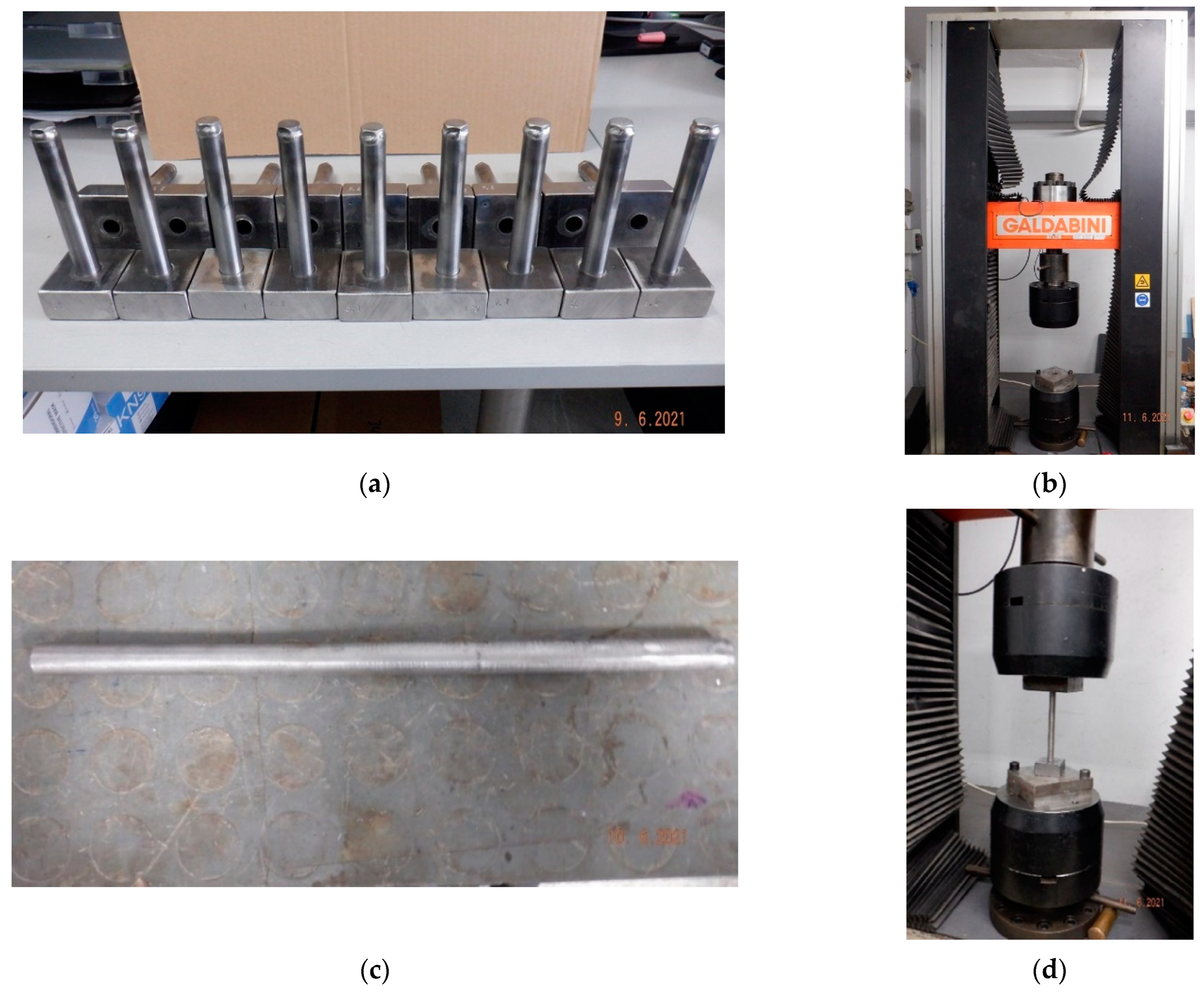
2.2. Test Tubesheet and Tube Specimens

For the experimental setup, hot rolled steel plate, P265GH (1.0425)/EN 10028-2 (METINVEST TRADEMETAL, SpA, Genoa, Italy), was used; its chemical composition and its mechanical properties are listed in

Table 3. Chemical composition % and mechanical properties of steel P265GH.

Type P265GH (1.0425)/EN 10028-2
Chemical Composition %
C	Mn	Si	P	S	Cu	Ni
Max 0.2	0.8–1.4	Max 0.4	Max 0.025	Max 0.01	Max 0.3	Max 0.3
Cr	Mo	Al	V	Nb	Ti	N
Max 0.3	Max 0.08	Min 0.02	Max 0.02	Max 0.03	Max 0.03	Max 0.012
Mechanical Properties
Yield strength (ReH) [MPa]		Min 255
Tensile strength (Rm) [MPa]		410–530
Elongation (A%)		Min 22

.

To cover the requirements for this project, eighteen (9 × 2) tubesheet specimens were prepared with nominal dimensions of 60 mm × 60 mm × 30 mm (Figure 1a). Nine multifactorial recipe runs were planned to be carried out, and each of them was duplicated. In addition, seamless steel tubes of material P215NL (1.0451)/EN 10216-4 (Ronconi SpA, Opera, Milan, Italy) were used; their chemical composition and their mechanical properties are listed in

Table 4. Chemical composition % and mechanical properties of steel P215NL.

Type P215NL (1.0451)/EN 10216-4
Chemical Composition %
C	Mn	Si	P	S	Cu	Ni
0.09	0.48	0.18	0.011	0.002	0.01	0.02
Cr	Mo	Al	V	Nb	Ti
0.03	0.01	0.028	0.001	0.001	0.003
Mechanical Properties
Yield strength (ReH) [MPa]		Min 225
Tensile strength (Rm) [MPa]		Min 360
Elongation (A%)		Min 25

. Similarly, eighteen (9 × 2) tube specimens were prepared with nominal dimensions of 19 mm (outer diameter) × 2 mm (wall thickness) × 150 mm (length) as shown in Figure 1b.

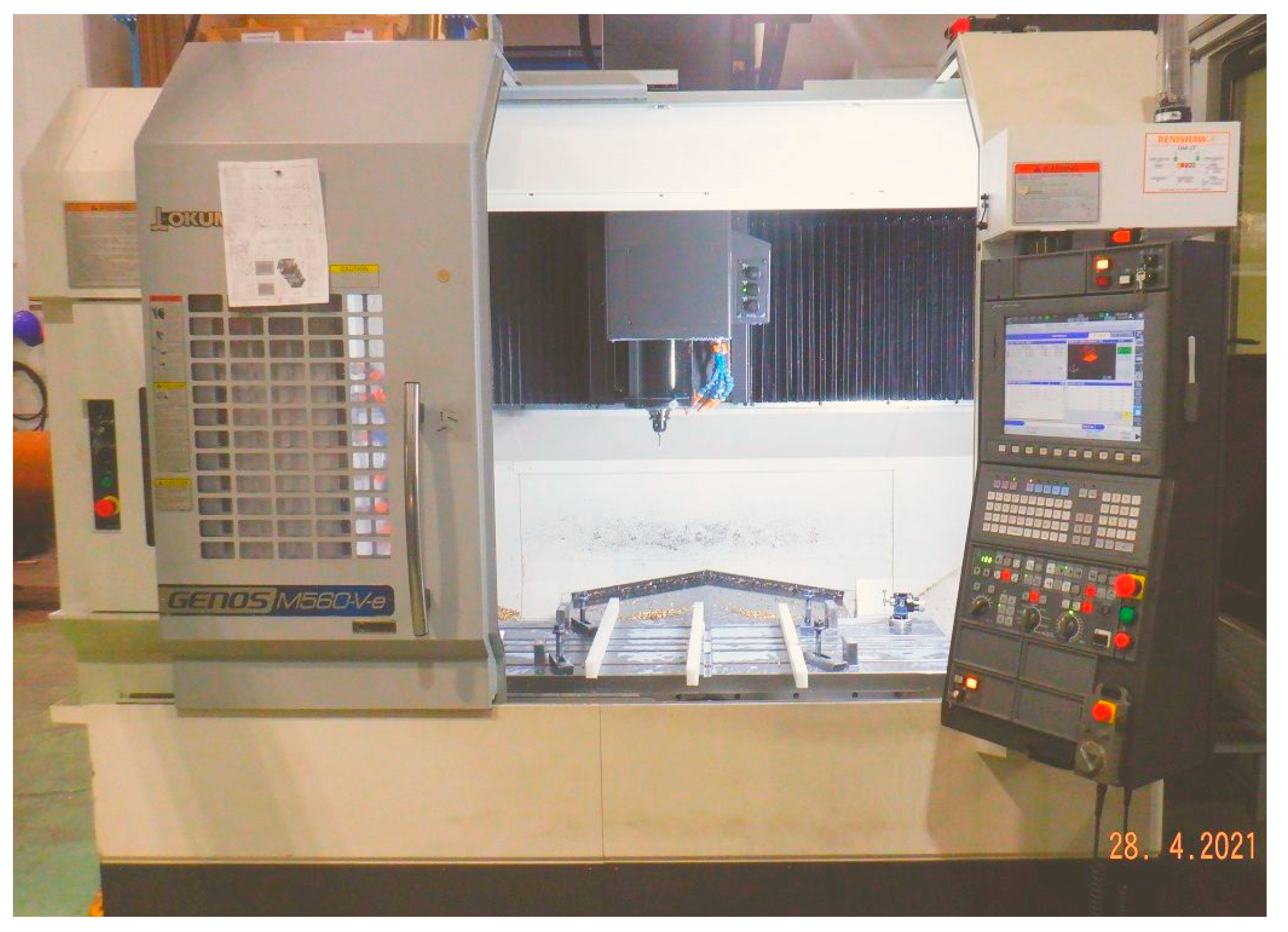
2.3. CNC Machining of the Test Tubesheet Specimens

Using a 2D CAD mechanical design software (AutoCAD, Autodesk, San Francisco, CA, USA), a technical drawing (Figure 2) was created which furnished all nine recipe layouts by configuring all four controlling factor combinations; each test tubesheet specimen was milled according to the standard Taguchi-type L₉(3⁴) OA in the saturated factorial arrangement.

Next, using a CAD/CAM mechanical design software (Fusion 360, Autodesk, San Francisco, CA, USA), 3D solid models were designed in order to generate the required G-code programs for the CNC milling treatment of the test tubesheet specimens (Figure 3). For the machining of the test tubesheet specimens, a 3-axis vertical milling CNC center (Genos M560-V-e, Okuma, Oguchi, Aichi, Japan) was employed which was also integrated with an OSP-P300MA-e (Okuma, Oguchi, Aichi, Japan) controller as depicted in Figure 4. The following three tools were selected to be examined for the machining trials of the test tubesheet specimens:

1.

DIJET Drill Bit Inserts (No. TEZ1900, Osaka, Japan): a carbide tool material with PVD coating (JC8050). Two indexable drill-bit inserts, with nominal diameter of 19 mm (Figure 5a), were utilized.

They were attached to a drill-body tool-holder (DIJET Drill Body, No. TEZD1900S25-MS). Each drill-bit insert was paired to complete each replicate set of nine workpieces as a preventive measure to curtail interloping variability due to local cutting process flaws.

2.

Sandvik Coromant Boring Inserts (ANSI code: TCGX 1.8 (1.5) 1L-WK 5015, Sandvik Coromant, Sandviken, Sweden): an uncoated carbide tool material. Two indexable boring inserts were utilized with corner radius and thickness dimensions of 0.3969 mm and 2.3812 mm, respectively. They were attached to a boring tool-holder (Sandvik Coromant Boring Bar, ANSI code: CXS-10-17 050TC09) and were mounted to a fine boring head adapter with a nominal accuracy of 0.002 mm (Figure 5b). Each boring insert was paired to process each replicate set of nine workpieces, again as a simple preventive measure in minimizing variability due to cutting process flaws.

3.

UOP T-slot Milling Cutters: solid High-Speed Steel (HSS) tool material (Roncadelle, Brescia, Italy). Two solid HSS T-slot milling cutters (Figure 5c), with cutting diameter and depth dimensions of 16.5 mm and 3 mm, respectively, were also outfitted with eight flutes. They were utilized to etch internal annular grooves on the tubesheet hole surfaces. Each T-slot milling cutter was paired to each separate set of nine workpieces. Upon completion of the machining process, the tubesheet specimens were crafted as shown in Figure 5d.

2.4. The Tube Expansion Process

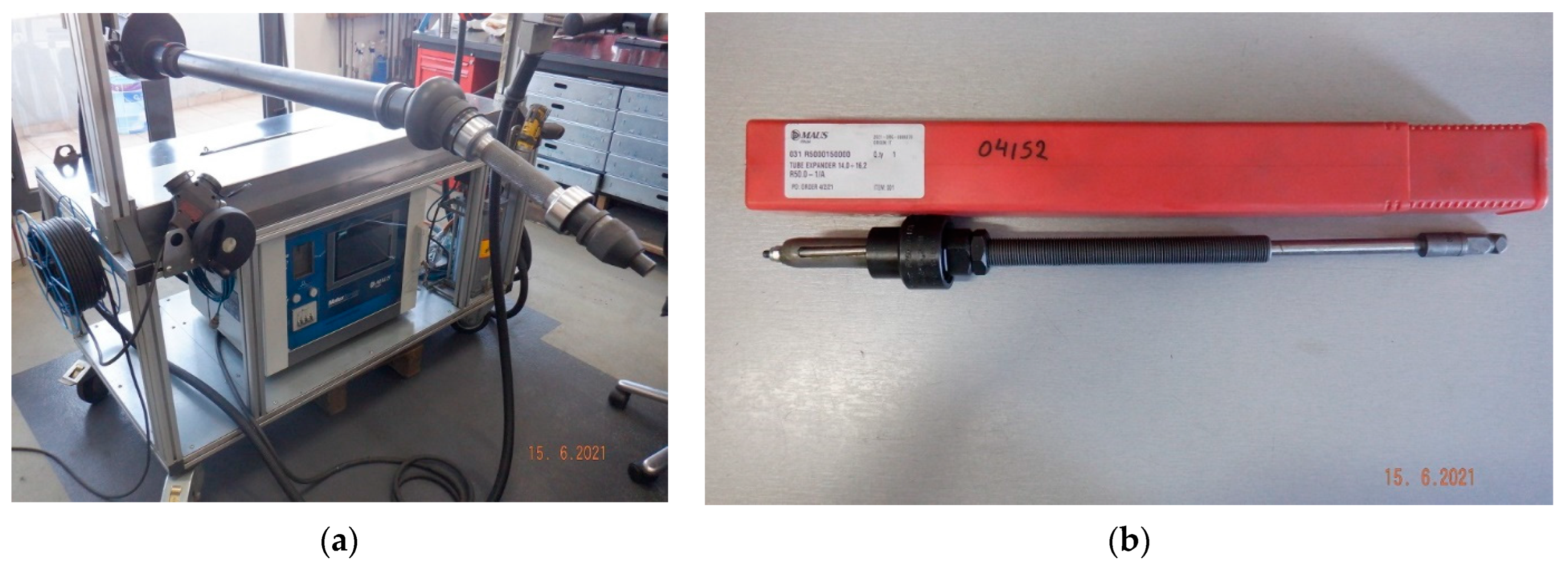
2.4.1. Tube Expanding Machine and Tube Expander Tool

For the tube expansion process, an electric tube expanding machine (Matex tsx-blu, Maus, Bagnolo Cremasco, Cremona, Italy) was employed (Figure 6a) which was comprised of the following components:

• A Matex tsx digital controller.
• A F/308-2 telescopic shaft which transmitted the rotational motion between the electric motor and the tube expander.
• An electric rolling motor (Matex R V4) which was composed of a brushless electric motor, and it was coupled to a mechanical gearbox with four speed options, i.e., 200, 300, 540, and 800 rpm.
• A PE900 foot switch control.

Table 5. Predetermination of proper tube expansion capability based on Equation (1).

Experiment No.	A	B	C	D	E	F	G
	Tubesheet Hole ID (mm)	Tube OD (mm)	Clearance (A Minus B) (mm)	Tube ID (mm)	Tube ID at Metal-To-Metal contact (D Plus C) (mm)	Tube Wall Thickness Reduction (%)	Expanded Tube ID [F% of (B-D) Plus E] (mm)
1.1	19.10	18.99	0.11	14.97	15.08	4	15.24
1.2	19.10	19.00	0.10	14.96	15.06	4	15.22
2.1	19.08	19.01	0.07	14.98	15.05	8	15.37
2.2	19.10	19.02	0.08	14.96	15.04	8	15.36
3.1	19.10	18.99	0.11	14.97	15.08	12	15.56
3.2	19.09	19.03	0.06	14.97	15.03	12	15.52
4.1	19.24	19.01	0.23	14.97	15.20	12	15.68
4.2	19.24	19.00	0.24	14.98	15.22	12	15.70
5.1	19.24	19.02	0.22	14.96	15.18	4	15.34
5.2	19.25	19.01	0.24	14.97	15.21	4	15.37
6.1	19.24	19.02	0.22	14.98	15.20	8	15.52
6.2	19.25	19.00	0.25	14.96	15.21	8	15.53
7.1	19.39	19.00	0.39	14.96	15.35	8	15.67
7.2	19.40	19.01	0.39	14.97	15.36	8	15.68
8.1	19.41	19.02	0.39	14.96	15.35	12	15.84
8.2	19.40	19.00	0.40	14.97	15.37	12	15.85
9.1	19.40	18.99	0.41	14.97	15.38	4	15.54
9.2	19.40	19.00	0.40	14.96	15.36	4	15.52

Table 5. Predetermination of proper tube expansion capability based on Equation (1).

Experiment No.	A	B	C	D	E	F	G
	Tubesheet Hole ID (mm)	Tube OD (mm)	Clearance (A Minus B) (mm)	Tube ID (mm)	Tube ID at Metal-To-Metal contact (D Plus C) (mm)	Tube Wall Thickness Reduction (%)	Expanded Tube ID [F% of (B-D) Plus E] (mm)
1.1	19.10	18.99	0.11	14.97	15.08	4	15.24
1.2	19.10	19.00	0.10	14.96	15.06	4	15.22
2.1	19.08	19.01	0.07	14.98	15.05	8	15.37
2.2	19.10	19.02	0.08	14.96	15.04	8	15.36
3.1	19.10	18.99	0.11	14.97	15.08	12	15.56
3.2	19.09	19.03	0.06	14.97	15.03	12	15.52
4.1	19.24	19.01	0.23	14.97	15.20	12	15.68
4.2	19.24	19.00	0.24	14.98	15.22	12	15.70
5.1	19.24	19.02	0.22	14.96	15.18	4	15.34
5.2	19.25	19.01	0.24	14.97	15.21	4	15.37
6.1	19.24	19.02	0.22	14.98	15.20	8	15.52
6.2	19.25	19.00	0.25	14.96	15.21	8	15.53
7.1	19.39	19.00	0.39	14.96	15.35	8	15.67
7.2	19.40	19.01	0.39	14.97	15.36	8	15.68
8.1	19.41	19.02	0.39	14.96	15.35	12	15.84
8.2	19.40	19.00	0.40	14.97	15.37	12	15.85
9.1	19.40	18.99	0.41	14.97	15.38	4	15.54
9.2	19.40	19.00	0.40	14.96	15.36	4	15.52

To conduct the tube-rolling process, a three-roller tube expander (R50.0-1/A, Maus, Bagnolo Cremasco, Cremona, Italy) was utilized with an available expansion accommodation ranging from 14.0 mm to 16.2 mm (Figure 6b).

2.4.2. Determination of the Proper Expanded Tube Inner Diameter

Before conducting the tube expansion process (Figure 7d), the required tube wall reduction percentage for each experiment was pre-evaluated to select suitable trial settings for the OA scheme. The relative tabulations from refs. [51,52] were adopted to complete the ensuing detailed calculations. Equation (1) from ref. [7] was used to allow a realistic pre-estimation of the tube inner diameters for the tube-rolling process (Table 5). Moreover, the tubesheet hole diameter, as well as the tube inner and outer diameters, were measured thrice each (Figure 7), for every replicated nine-run set of experiments, and their mean values were recorded. The tolerance limits of the expanded tube inner diameters for each individual experiment were determined to be within ±0.05 mm.

Expanded tube ID = (Tubesheet hole ID − Tube OD) + Tube ID + (Tube wall thickness × 2) × (% Tube wall reduction)

(1)

Because of the criticality of a proper specimens’ preparation in ensuring trustworthy test-joint strength measurements, the grooves on the tubesheet-hole walls, along with the tube inner and outer surfaces, were pre-treated to rid of any surface blemishes, such as burrs, grease, oil residue, rust, or dirt. The finalized torque settings which were applied during the tube-rolling process and their expected tube wall thickness reduction percentage are listed in

Table 6. Torque values used for tube rolling.

Tube Wall Thickness Reduction (%)	Torque (Nm)
4	8
8	12
12	15

.

2.5. Joint Strength Measurements

Before commencing the tube push-out testing procedure, the tube ends of the tube specimens were sealed with welded plugs as depicted in Figure 8a. A tensile/compressive testing machine (CTM/50, Galdabini, Cardano al Campo, Varese, Italy) was utilized (Figure 8b) to perform the tube push-out tests. The testing machine was integrated with GraphWork 5.0 test software which recorded the applied loads on the tubes during the push-out testing process. Moreover, a round steel bar of material S355 (Figure 8c), with nominal diameter and length dimensions of 14 mm and 295 mm, respectively, was inserted into the tube end to direct the axial load transmission (Figure 8d); it forced the tube out of the tubesheet hole to the point of mechanical failure of the joint or the tube (Figure 8e,f). The push-out tests were carried out at a constant crosshead speed of 5 mm/min. After the axial tube-displacement process was initiated, the applied load was monitored and recorded by the testing equipment. The maximum load was applied at the start of the displacement cycle and then it was gradually decreased. The terminal condition of the tube-to-tubesheet specimens exiting the push-out testing is demonstrated in Figure 8g. Duplicate joint strength measurements were obtained for the nine-run tube-to-tubesheet specimens.

2.6. Theoretical Aspects and Computational Aids

The basic matrix arrangement of the L₉(3⁴) OA with its coded 3-level settings is shown in Figure 9 for a duplicated output R with its nine-entry replicate vectors R1 and R2, respectively. The coded controlling factors in the input nine-run configuration are denoted as A, B, C, and D, respectively.

In Figure 10, the two separate data reduction steps are shown that generate the central tendency measure (mean value—M) and the dispersion measure (SNR) for the duplicated data entries of Figure 9.

To estimate the SNR value for each run, the pertinent formula for a general ‘larger-is-better’ quality characteristic is given by the Taguchi-based transformation expression—suited here for estimating the variability of duplicate data entries:

$${\mathrm{S}\mathrm{N}\mathrm{R}}_i=-10 \mathrm{l}\mathrm{o}\mathrm{g}\left(\frac{1}{2}\sum _{j=1}^2\frac{1}{r_{ij}^2}\right)\mathrm{w}\mathrm{i}\mathrm{t}\mathrm{h} 1\le i\le 9$$

The basic Taguchi-recommended data preparation, analysis, and presentation were performed by the statistical software MINITAB 19.0 (State College, PA, USA), which provided the L₉(3⁴) OA trial planner to schedule the duplicated and saturated multifactorial runs. The ‘STATS/DOE/ Taguchi’ module offered the integrated statistical solution for the dual screening and optimization task by separately arriving at a prediction for the joint strength location (mean of means) and dispersion (mean of SNR) values. Thus, the non-linear response tables and graphs for both the mean and SNR response were generated. The classic ANOVA and regression analysis treatments on the unprocessed joint strength replicates were also employed to: (1) weigh the variance of the individual controlling factors against the residual error, and (2) obtain the coefficients of regression, which give a statistical measure of the magnitude of the potentially non-linear effects. The between-replicates agreement is easily assessed by drawing a simple goodness-of-fit least-squares line plot to evaluate the correlated relationship and possible deviation between the two collected joint strength replicate vectors. In the case of substantial observed deviation, additional replicate runs would be scheduled, and the assessment process would be repeated to determine the variability status between the replicated runs. Boxplots are also drawn to portray in a robust manner the variability within each factor setting and to visually contrast the effects among different settings.

The algorithmic data analysis of the joint strength OA-dataset is also explored using several facilities from the statistical freeware platform R (v. 4.2.2) [53]. The R-package ‘randomForest’ (v. 4.7-1.1) was employed to perform the Random Forest regression analysis. The mean squared error and the node purity were recovered from the assorted R-function ‘importance()’. The partial dependences of the four controlling factors on the joint strength were graphically obtained using the R-function ‘partialPlot()’. The prediction of the confirmation-run data was evaluated using the R-function ‘predict()’ and in comparison to the optimal screening/optimization combo-solution. The optimal number of variables which were randomly sampled as candidates at each split was tuned by the R-function ‘tuneRF()’—the step factor to inflate/deflate the number of trees was set at 0.5 and the number of trees was set at 1000.

3. Results

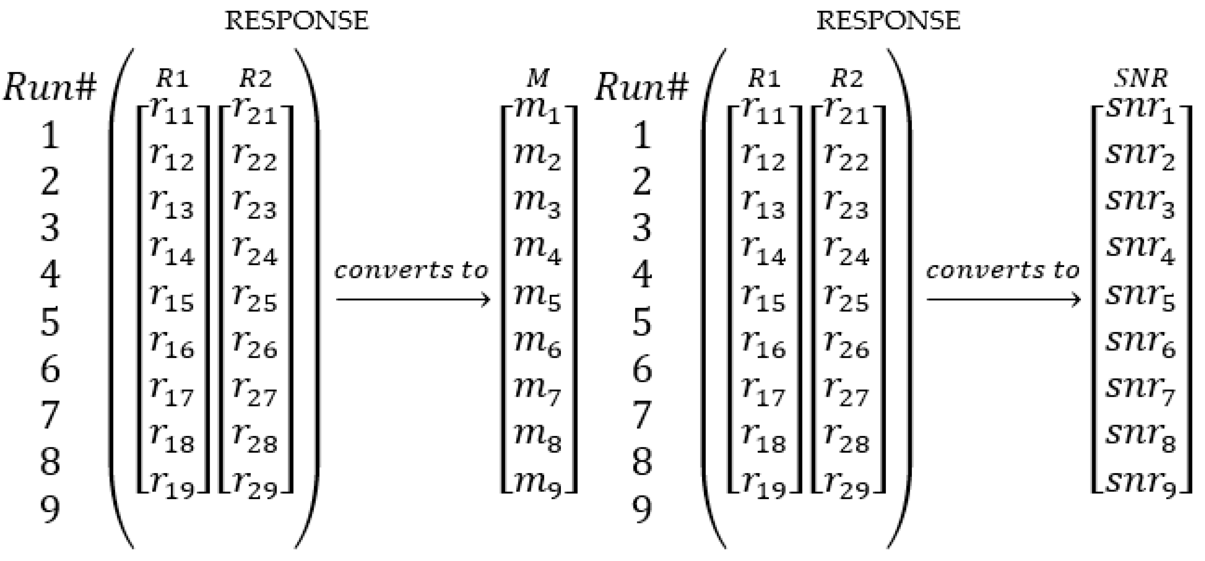
3.1. Joint Strength Statistical Analysis Using Response Graphs and Tables

The duplicated nine-run measurements of the joint strength response along with a calculation of their mean and SNR values [54] are listed in

Table 7. Duplicated dataset, mean, and SNR estimations of the joint strength.

Run#	Joint Strength (N) Trial #1	Joint Strength (N) Trial #2	Joint Strength Mean (N)	SNR-Joint Strength (dB)
1	17,880.00	16,597.50	17,238.75	84.71
2	37,552.50	38,400.00	37,976.25	91.60
3	45,371.25	44,913.75	45,142.50	93.09
4	31,263.75	29,811.25	30,537.50	89.70
5	11,935.00	13,500.00	12,717.50	82.04
6	39,768.75	39,330.00	39,549.38	91.94
7	17,523.75	18,288.75	17,906.25	85.05
8	38,662.50	37,706.25	38,184.38	91.64
9	24,318.75	26,525.00	25,421.88	88.08

. The joint strength means values range from 12,717.50 N to 45,142.50 N which indicates that there is noticeable variation among the nine runs. On the other hand, SNR values exhibit less variation since their range is confined between 82.04 dB and 91.94 dB. From the joint strength response table for means (

Table 8. Response table for joint strength mean (N).

Level	Clearance	Number of Grooves	Groove Depth	Tube Wall Thickness Reduction
1	33,452.50	21,894.17	31,657.50	18,459.37
2	27,601.46	29,626.04	31,311.87	31,810.62
3	27,170.83	36,704.58	25,255.42	37,954.79
Difference	6281.67	14,810.42	6402.08	19,495.42
Rank	4	2	3	1

), it is the tube wall thickness reduction that appears to cause the greatest disturbance on the joint strength mean response. The maximum difference between settings was calculated at 19,495.42 N. Substantial variation among settings is also attributed to the number of the grooves—a maximum difference between settings is estimated at 14,810.42 N.

The remaining two factors, the clearance and the groove depth, are behaving as of a lesser importance—at a similar effect magnitude between them. According to the response graph for the joint strength mean, the optimal setting of the tube wall thickness reduction is 12% and the respective optimal setting of the number of grooves is three. Similar observations may be drawn from the response table (

Table 9. Response table for the joint strength SNR (dB).

Level	Clearance	Number of Grooves	Groove Depth	Tube Wall Thickness Reduction
1	89.80	86.49	89.43	84.94
2	87.89	88.42	89.79	89.53
3	88.26	91.04	86.73	91.47
Delta	1.91	4.55	3.06	6.53
Rank	4	2	3	1

) for the joint strength SNR. However, the discrepancies between settings are relatively smaller for the SNR estimations. The tube wall thickness reduction and the number of the grooves elicit a maximum difference in the joint strength mean SNR values of 6.53 dB and 4.55 dB, respectively. Overall, it may be remarked that both factors cause minor disturbance on the mean SNR response of the joint strength. Similarly, the main effects plot for the joint strength mean SNR shows that the corresponding optimal settings are exhibiting the same pattern as in the main effects for the means plot, i.e., optimally set at 12% for the former and three for the latter.

To proceed with the analysis part, the statistical significance of the outcomes is obtained from the ANOVA treatment. As expected, the two data reduction steps have each separately down-sized the duplicated form of the original datasets—mean and SNR estimations—to a virtual ‘unreplicated response’ form. Additionally, the experimental OA-plan was decided to be fully loaded with controlling factors (‘saturated’ condition). Hence, the usefulness of the ANOVA is restricted to offering only a relative strength evaluation among the factorial contributions. This is because in the saturated-unreplicated form, an OA sampler does not permit significance estimations in the absence of a residual error. This is observed in both ANOVA tables, for means and SNR estimations (

Table 10. ANOVA treatment for the response means of the joint strength.

Factor	DF	adj SS	adj MS	F-Value	p-Value	Contribution (%)	Rank
Clearance	2	73,879,463	36,939,731	*	*	6.86	4
Number of Grooves	2	329,236,085	164,618,042	*	*	30.57	2
Groove Depth	2	77,786,815	38,893,408	*	*	7.22	3
Tube Wall Thk. Reduction	2	596,077,932	298,038,966	*	*	55.35	1
Error	0	*	*			*
Total	8	1,076,980,294				100.00
Model Summary
S    R-sq       R-sq (adj)    R-sq (pred)
*    100.00%       *             *

*: no value available.

and

Table 11. ANOVA treatment for the response SNR estimations of the joint strength.

Factor	DF	adj SS	adj MS	F-Value	p-Value	Contribution (%)	Rank
Clearance	2	6.146	3.073	*	*	5.05	4
Number of Grooves	2	31.321	15.661	*	*	25.74	2
Groove Depth	2	16.777	8.389	*	*	13.79	3
Tube Wall Thk. Reduction	2	67.423	33.712	*	*	55.42	1
Error	0	*	*			*
Total	8	121.668				100.00
Model Summary
S    R-sq       R-sq (adj)    R-sq (pred)
*    100.00%       *             *

*: no value available.

). Despite that, it is still worthwhile to contemplate the leading contributions, in terms of mean sum of squares calculations. Actually, the tube wall thickness contributes about 55% to the total sum of the mean sums of squares for both estimator treatments—mean and SNR joint strength response. Similarly, the number of grooves contributes to the mean and SNR sums of squares of the joint strength response about 30.57% and 25.74%, respectively. Even though there is not available information from either the statistical significance or the goodness-of-fit computations to assess the status of the predictions, nevertheless, a qualitative comparison between the data-reduced (mean and SNR) joint strength variable with the simplistic response graph and response table results seems to lead to an agreement.

Of course, it is always beneficial to perform a regular ANOVA treatment, i.e., without any intermediate data-reduction step on the joint strength replicates. In

Table 12. Stepwise ANOVA results for unprocessed response joint strength dataset.

Source	DF	adj SS	adj MS	F-Value	p-Value
Regression	7	2,153,533,744	307,647,678	423.04	0.000
A	1	118,378,008	118,378,008	162.78	0.000
B	1	658,045,326	658,045,326	904.86	0.000
C	1	122,960,013	122,960,013	169.08	0.000
D	1	1,140,213,813	1,140,213,813	1567.87	0.000
A∗A	1	29,380,917	29,380,917	40.40	0.000
C∗C	1	32,613,617	32,613,617	44.85	0.000
D∗D	1	51,942,050	51,942,050	71.42	0.000
Error	10	7,272,359	727,236
Lack-of-Fit	1	426,844	426,844	0.56	0.473
Pure Error	9	6,845,515	760,613
Total	17	2,160,806,104
Model	Summary
S	R2	R2 (adj)	R2 (pred)
852.78	99.66%	99.43%	98.89%

A = Clearance, B = Number of Grooves, C = Groove Depth, D = Tube Wall Thickness Reduction.

, the stepwise ANOVA comparison outcomes are in close proximity to those from the ANOVA treatment for the mean-reduced response dataset (Table 10). All four controlling factors appear to be statistically significant (p < 0.001), even for a Bonferroni-corrected family-wise error of 0.01. Furthermore, the adjusted coefficient of determination (adj R²) and the coefficient of determination for prediction (pred R²) were estimated at 99.43% and 98.89%, respectively, which implies an overall satisfactory interpretation of the explained variation. There is no lack of fit and the stepwise selection terms were determined with the same error rate α ‘to enter’ and ‘to remove’. Only the quadratic term which was related to the number of the grooves was excluded from the model. To differentiate the effects of the linear and quadratic terms in explaining the total variation, the coefficients of regression are indispensable. In

Table 13. Stepwise regression coefficients for the joint strength response dataset.

Term	COEF	SE COEF	T-Value	p-Value	VIF
Constant	31,907	532	60.00	0.000
A	−3141	246	−12.76	0.000	1.00
B	7405	246	30.08	0.000	1.00
C	−3201	246	−13.00	0.000	1.00
D	9748	246	39.60	0.000	1.00
A∗A	2710	426	6.36	0.000	1.00
C∗C	−2855	426	−6.70	0.000	1.00
D∗D	−3604	426	−8.45	0.000	1.00
Regression	Equation:
Joint Strength	=	31907 − 3141 A + 7405 B − 3201 C + 9748 D + 2710 A2 − 2855 C2 − 3604 D2

A = Clearance, B = Number of Grooves, C = Groove Depth, D = Tube Wall Thickness Reduction.

, it is tabulated both regression coefficients, for the linear and the quadratic components for all four controlling factors. It is re-affirmed that the joint strength behaves linearly against the number of the grooves, while the rest of the controlling factors also uphold a quadratic component. For the leading effects, it is the linear part of the effect of the tube wall thickness reduction and the number of grooves that is statistically prevailing. It is additionally noted that the variance inflation factor (VIF) estimations (MINITAB 19.0, State College, PA, USA), for all four parameters, were equal to 1.0 which signifies that there is no issue of multicollinearity between the factorial relationships in the prediction model. This was partly accomplished by standardizing the factorial levels to end point model values of −1 to 1.

In Table 13, the regression equation for the joint strength dependencies is also given. To decide whether to retain the weaker predictors, a best-subsets regression was carried out. As it is shown in

Table 14. Best subsets regression (B and D participate in all models).

Total Variables	R2	R2 (adj)	PRESS	R2 (Pred)	Mallows’s CP	S	A	C
3	88.9	86.5	323,492,722.0	85.0	15.7	4136.8		X
3	88.7	86.3	374,906,004.8	82.6	16.2	4176.2	X
4	94.4	92.7	199,192,722.4	90.8	5.0	3053.5	X	X

A = Clearance, B = Number of Grooves, C = Groove Depth, D = Tube Wall Thickness Reduction.

, while maintaining the two leading regressors in all tested models (the number of grooves and the tube wall thickness reduction), it was found that retaining also the clearance and the groove depth would also maximize the adjusted and predicted R², whereas the Mallows’s Cp statistic (MINITAB 19.0) is minimized to a value of 5.0, which signifies that there is no appreciable bias in the finalized model selection (C_p = 5.0 < 2p = 8).

3.2. Proposed Optimal Solution for the Screening/Optimization of the Joint Strength

The optimal parameter settings have been easily identified from the main effects plots for the means and the SNR values (Figure 11). The optimal adjustments that maximize the performance of the tube-to-tubesheet joint strength, after the completion of the combined Taguchi screening and optimization study, are the following:

• Tube wall thickness reduction at level 3 (12%).
• Number of grooves at level 3 (Three).
• Groove depth at level 2 (0.40 ± 0.02 mm).
• Clearance at level 1 (0.10 ± 0.02 mm).

It is immediately apparent that the above combination of parameters does not match any of the nine executed recipes that were originally planned by the L₉(3⁴) OA sampler (Table 2). It is also noted that the groove depth is finally adjusted in accordance with the TEMA standards [7,51,52], which specify that the deep annular grooves are to be machined at approximately 0.40 mm. This is a practical intervention in view of the fact that the magnitude of the influence of the groove depth is, arguably, mildly active even if it appears to be statistically significant.

The next step was to calculate the predicted value for the maximum joint strength using the Taguchi analysis module from the statistical software MINITAB 19.0 (State College, PA, USA). In

Table 15. Predicted values for the maximum performance of the joint strength.

Prediction Method	Predicted Maximum Joint Strength
Taguchi Method	Mean = 51,199.00 N (s = 729 N) SNR = 96.1 dB
Stepwise Regression	51,307 N

, the predicted value of the joint strength from the Taguchi method as well as its predicted value from the stepwise regression equation are compared. The linear regression equation was formed from the statistically significant coefficients (Table 13) which also included a statistically important constant term. The linear regression equation has been given explicitly in a standardized formulation at the bottom of Table 13. From Table 15, it is inferred that the predictions from the Taguchi method and the stepwise regression are fairly proximate. However, from Table 7, no run produced such measurement to propel the joint strength performance so high. The joint strength observations ranged between 11,935.00 N and 45,371.25 N. The Taguchi method and the stepwise regression treatments offered maximum joint strength prediction values of 51,199.00 N and 51,307 N, respectively, which is a surprisingly advantageous finding.

3.3. Confirmation Run for the Optimal Parameter Settings

The optimal layout of the specimens (the 10th factorial recipe), which is prepared on the suggested parameter adjustments from the previous subsection, is re-drawn and is shown in Figure 12. The confirmation run was comprised of five pairs of machined tubes and tubesheets, which are shown in Figure 13. Thus, the confirmation run was replicated five times. The collected measurements from the confirmation experiment are listed in

Table 16. Joint strength observations from the confirmation trial runs.

Run#	Max. Joint Strength (N)	Max. Joint Strength Mean (N)
1	44,013.75	$\stackrel{-}{x}$ = 43,861.75 ($\stackrel{-}{s}$ = 424.45) 95% C.I. (43,334.73, 44,388.77) Coefficient of Variation = 0.0098
2	43,218.75
3	44,392.50
4	43,813.75
5	43,870.00

.

Even though only five confirmation runs were programmed to constitute an initial test sample, the tapered 95%-confidence-interval estimation (Table 16) hinted that no additional confirmation-run samples would be meaningful at this stage. The notion of lean thinking also extends to minimizing the confirmation trials, if the trends are already practically explainable and there is a firm grasp on how joint strength variability is distributed among its accounted sources. Moreover, this was attested because of the accompanying very low value of the coefficient of variation of the confirmed joint strength performance (0.0098). However, the discrepancy between the predictions due to the Taguchi method and the stepwise regression analysis, on one hand, and the confirmation-run joint strength mean response values, on the other, was calculated at a relative percentage of about 14%. While the complexity of the physical phenomena behind this mechanical process is known to be high, and in part, it could justify such realistic deviation, particularly under the espoused condition of the ‘lean-green-driven’ (miniaturized) experimentation, in the Discussion section there will be further exploration about the cause of such discrepancies. Conversely, the confirmation-run joint strength performance matches fairly close to the maximum observable joint strength measurement in the OA trials which was found to be 45,371.25 N (Table 7). Thus, their difference may be viewed now more tolerable at the relative percentage of 3.3%. It is concluded that this study might have produced useful empirical relationships, but an alternative non-statistical treatment might provide insight from a different angle. This last issue will be discussed in the next section.

4. Discussion

Although the maximum trial observation was in accord to the mean value of the joint strength data from the confirmation-run sample, their departure of the predicted mean from the OA-screening/optimization exercise was noticeable. This might be a matter for broader exploration. From the previous section, it was found that all parameters may be taken as active in modulating the integrity of a tube-to-tubesheet expanded joint. In spite of being all statistically significant, the four parameters could be virtually split into two distinct groups based on their magnitudes of their influence. The four examined parameters, (1) the clearance between the tubesheet hole diameter and the tube outer diameter, (2) the number of grooves in the tubesheet hole, (3) the groove depth in the tubesheet hole, and (4) the tube wall thickness reduction, were shown to have a linear component that was statistically significant. These four controlling factors were nominated to be a group of proper candidates for this factorial screening and parameter optimization because they are commonly mentioned by the TEMA standards [7]; as also, they were recommended from previous published research [8,9,10,11,12,23]. Furthermore, it was found that in terms of magnitude, the quadratic terms were of lesser importance, yet statistically significant, to three out of the four examined parameters: (1) the clearance between the tubesheet hole diameter and the tube outer diameter, (2) the groove depth in the tubesheet hole, and (3) the tube wall thickness reduction.

A post-screening assessment could be initiated by depicting the four controlling factors in boxplots for each individual controlling factor to emphasize the visual aspect of their variability owing to different settings. In Figure 14, the corresponding four boxplots have been prepared (MINITAB 19.0, State College, PA, USA). It is immediately discerned that only the tube wall thickness reduction could amass distinguishable variation across settings. A linear dependence emerges which is solely framed by the two operating endpoints of this factor. The second (middle) setting merely overlaps across both end settings. The rest of the controlling factors do not pass the test of visual evidence. Perhaps, their influence on the joint strength response is dubious; their confidence intervals for their medians are overlapping across all settings. Equally striking is the asymmetric location tendencies in the data sample median values as exposed by individual settings.

No particular side is favored in the numerical accumulation of the observations; they are predominantly asymmetric across all four factors. A plausible question would be whether any additional trial runs would refine more the precision around the magnitude estimation of the effects and, hence, would assist to expediting the practical aspect of the profiling process. To check consistency in the duplicated trials of the joint strength experiments, the two replicates are regressed against each other (Figure 15). It results in a symmetrical line fitting—the fitted line slope is 1.03—and the adjusted coefficient of determination is estimated at 98.7%. It is inferred that there is no immediate concern to conduct more replications or selectively augment the volume of observations.

It is useful to also obtain an alternative prediction from a classic algorithmic solver such as the Random Forest. The trial outcomes from running the Random Forest module 10 times are summarized and tabulated in

Table 17. Random Forest trial statistics to fit the saturated L₉(3⁴) OA joint strength dataset.

	N	Mean	Std. Deviation	Std. Error Mean	95% Confidence Interval
					Lower	Upper
MSR	10	17,843,680	1,115,982	352,904	17,045,354	18,642,006
VE	10	85.13	0.93	0.29	84.47	85.80
MSE A	10	8.03	0.75	0.24	7.50	8.57
MSE B	10	25.06	0.61	0.19	24.62	25.50
MSE C	10	3.74	0.99	0.31	3.03	4.45
MSE D	10	33.21	0.95	0.30	32.53	33.88

MSR = Mean of Squared Residuals, VE = Variation Explained (%), MSE = Mean Squared Error: A = Clearance, B = Number of Grooves, C = Groove Depth, D = Tube Wall Thickness Reduction.

(IBM SPSS v.29, Armonk, NY, USA). The precision of the predictions is deemed adequate. This was determined by evaluating the descriptive statistics for a start-up sample. The Random Forest quantities of statistical interest were the mean of squared residuals (MSR), the percentage of the explained variation (VE), and the mean squared error (MSE) for the four controlling factors. Then, the descriptive statistics were re-evaluated by adding in the final sample (n = 10), an additional batch of five prediction runs from executing the Random Forest module. The mean difference estimates between the two sampling phases were found to converge to the listed precision with an experimental test power of 0.95. Thus, no further Random Forest solver runs were deemed necessary.

To achieve such a stable solution, ‘the number of trees to grow’ was set at a relaxed modelled value of 1000 trees in the R-package ‘randomForest’ (v. 4.7-1.1). However, the Random Forest module often converged to a solution that implemented as low as 100 trees, as shown in Figure 16. The number of variables randomly sampled as candidates at each split (m_try) was determined upon minimization of the ‘out-of-bag’ error (OOB). From Figure 17, the optimal m_try number is 4 variables. Consequently, the partial dependence plots for tracking the behavior pattern of the joint strength, in terms of the four screened factors, are shown in Figure 18. It is now unequivocal that primarily the tube wall thickness reduction and, next, the number of grooves in the tubesheet hole, might stimulate enough variability to be classified as active influences. Thus, they might pass the screening filter phase and proceed next to undergo the optimization drill. In agreement with the explained variation estimation (Table 17), the Random Forest regression manages to attribute 85.13 % of the variability to the four profiled factors with an assorted increasing node purity (mean of squared residuals) of 17,843,680. From the derived Random Forest importance measures, the fluctuation of the mean squared error is essentially identified to the tube wall thickness reduction (33.21%) and the number of grooves in the tubesheet hole (25.06%).

The prediction outcomes from the ten Random Forest solver runs, using as test data the confirmation-run sample from Table 16, were collected. Upon summarizing, data were found to be represented by a mean value of 40,240 N (standard error for the mean = 28.5 N) and a 95% confidence interval of (40,176 N, 40,305 N). This time, the percentage deviation is only 8.3% which improves over the initial application of the Taguchi approach (14%). The overall prediction outlook of the joint strength integrity is rendered more realistic by the involvement of the Random Forest data analysis. The prediction estimation improves even more when only the two active effects are retained in the final model, i.e., the tube wall thickness reduction and the number of grooves in the tubesheet hole. In this case, the estimated prediction (based on the response table for joint strength means—Table 8) becomes 45,251 N which deviates only 3% from the confirmation-run sample.

Overall, this work offered a compromised solution from four different data analysis routes: (1) Taguchi’s response graphs/tables, (2) ANOVA treatment, (3) regression analysis, and (4) Random Forest application. This was considered imperative given the realistic expectations for carrying out this research, i.e., in limited time and minimal budget, ensuring that it mimics the urgent requirements of a ‘lean-and-green’ industrial project. The limited number of tube push-out tests was critical to project execution because the measurements were subcontracted to a nationally accredited testing laboratory in order to ensure accurate and valid observations. This was materialized by using the fractional factorial sampling tactic, keeping replication to a minimum and finally performing confirmation runs to a restricted number. Nevertheless, a conceived factor such as the surface finish of the tubesheet holes may induce a detectable effect on joint strength [7,9]. This factor was not examined in the present research. According to the TEMA standards [7], it is stated: “a smooth tubesheet hole can provide a pressure tight joint at a lower level of wall reduction, but a rough tubesheet hole provides more mechanical strength than a smooth tubesheet hole” (pp. 10–31). Since rough tubesheet holes and strong joints may be related, extending this research would uncover valuable links to enhancing the joint integrity on the particular production materials as used in this study.

There are several practical implications that become evident upon completion of such a study. First, it has been demonstrated that it is feasible to treat the multifactorial screening and optimization problem of improving the joint integrity for a tube-and-shell heat exchanger. According to the latest exhaustive review on the phenomena surrounding the failure mechanisms of the tube-to-tubesheet joints, an application of a data-centric engineering approach is a new perspective; it has never been dealt with in the past even though the problem is old and the operational maladies it causes are well established [15]. The practicality of the proposed method makes it easily deployable where it is needed the most—at the assembly line. Since different types of materials and designs are used for different types of heat-exchanger brands, the proposed methodology appears useful and versatile to the traditional heat-exchanger fabrication processes in general because: (1) it is affordable to be locally and directly carried out at the assembly floor, (2) it is adaptable to execution for any customized workflow parameters, (3) it is convenient to rapidly organize at the point of application, and (4) it requires no new knowledge to be pre-assimilated in order to be implementable. As stated in Thekkuden et al. [15], even today, the old problem of heat-exchanger tube-to-tubesheet joint failures demands an intensive leak inspection program to ensure long-lasting equipment functioning. There is an enormous investment loss from reduced capacity due to heat-exchanger failures. Modern lean-and-green approaches are available to prevent joint fabrication defects by providing quick and cheap information on demand at the point of interest, on the shop floor. The empirical modeling assists the production engineers to promptly focus on those controlling factors that should receive immediate attention for a more resilient equipment operation.

The proposed data-centric engineering approach have surfaced the inherent complexity of the underlying mechanical phenomena which are easily manifested after a simple graphical analysis; the joint strength is behaving mainly in a non-normal fashion for most screened parameters. This is a complication that a process engineer finds immensely challenging to handle. The study also showed that even though all investigated controlling factors were found statistically significant, practically, two of them actually controlled the maximization of the joint integrity. This simplifies the problem for a production engineer by halving the amount of effort—in the specific case study—in searching to adjust the tube-to-tubesheet joint performance. The opportunity to diagnose the situation at hand by a one-time ‘check-and-correct’ approach is always appreciated in a fast-paced manufacturing environment.

5. Conclusions

A ‘lean-and-green’ approach was developed in this study to explore the simultaneous non-linear screening and optimization of the integrity of a tube-to-tubesheet expanded joint in the fabrication of a shell-and-tube heat exchanger. The Taguchi method facilitated the quick uncovering of the four investigated influences. Optimal parameters for the maximum joint strength on a tube-to-tubesheet expanded joint were obtained. The experimental results were evaluated by using the ANOVA treatment (on both raw and reduced duplicated responses). The estimated coefficients of the controlling factors were obtained using a regression analysis. The factorial profiling was characterized by low unexplainable dispersion which resulted in all four examined factors appearing significant often in their linear and quadratic terms. Practically, as was also checked with a Random Forest regression analysis, the factors could be discerned in two groups. The important group was identified to tube wall thickness reduction and the number of the grooves. In a nutshell, the optimal settings for all considered factors are suggested as follows:

• Tube wall thickness reduction at level 3 (12%).
• Number of grooves at level 3 (Three).
• Groove depth at level 2 (0.40 mm).
• Clearance at level 1 (0.10 mm).

According to the results of the ANOVA statistical analyses, it was found that the tube wall thickness reduction has the highest influence on joint strength (at 55.17%), followed by the number of grooves (at 30.47%), the groove depth (at 7.20%), and the clearance (at 6.84%).

Based on the comparisons of the confirmation-run results with both the predicted values from the Taguchi method and the regression equation, the deviation may be as high as 14% which is not unusual in these types of experiments. This was due to the fact that the collected joint strength dataset was often deviating from normality when segmented in terms of settings. The Random Forest method aided in ensuring the pinpointing of the two dominant effects. Overall, the Taguchi parameter design can be considered successful since the predictions of the Random Forest algorithm are close enough to the confirmation-run test summary results within 3%. The comparison between the experimental results of the confirmation test and the Experiment No. 3 shows that for a groove depth of over 0.40 mm, there is no significant effect on the joint strength since only a minute portion of the tube metal penetrates into the grooves during the tube expansion process. All the above results showed that the Taguchi method accelerated the optimization of the joint strength of a tube-tubesheet expanded joint. The fractional factorial DOE approach could be extended in the future to include the following:

• Further testing would be informative in investigating the joint leakage by exposing the joint in either pneumatic or hydraulic pressure tests; joint leak tightness cannot be measured directly by push-out testing.
• Further testing is needed to be conducted to study the influence of surface finish of the tubesheet holes on joint strength and joint leak tightness.
• The effect of a five-roller tube expander and a tube expander which incorporates three expansion rollers with three flare rollers on joint strength and joint leak tightness would be beneficial.

References

1. Nemati, H.; Ardekani, M.M.; Mahootchi, J.; Meyer, J.P. Fundamentals of Industrial Heat Exchangers: Selection, Design, Construction, and Operation; Elsevier: Amsterdam, The Netherlands, 2023. [Google Scholar]
2. Nitsche, M.; Gbadamosi, R.O. Heat Exchanger Design Guide: A Practical Guide for Planning, Selecting and Designing of Shell and Tube Exchangers; Butterworth-Heinemann: Amsterdam, The Netherlands, 2015. [Google Scholar]
3. Kakaç, S.; Liu, H.; Pramuanjaroenkij, A. Heat Exchangers: Selection, Rating, and Thermal Design, 4th ed.; CRC Press: Boca Raton, FL, USA, 2020; pp. 4–6. [Google Scholar]
4. Gulyani, B.B. Estimating Number of Shells in Shell and Tube Heat Exchangers: A New Approach Based on Temperature Cross. ASME. J. Heat Trans. 2000, 122, 566–571. [Google Scholar] [CrossRef]
5. Bell, K.J. Heat Exchanger Design for the Process Industries. J. Heat Transfer. 2004, 126, 877–885. [Google Scholar] [CrossRef]
6. Master, B.I.; Chunangad, K.S.; Boxma, A.J.; Kral, D.; Stehlík, P. Most Frequently Used Heat Exchangers from Pioneering Research to Worldwide Applications. Heat Trans. Eng. 2006, 27, 4–11. [Google Scholar] [CrossRef]
7. Standards of the Tubular Exchanger Manufacturers Association, 10th ed.; Tubular Exchanger Manufacturers Association, Inc.: New York, NY, USA, 2019; pp. 5.7-11–5.7-12, 10–31.
8. Yokell, S. Heat exchanger tube-tubesheet connection. Chem. Eng. 1982, 75, 78–94. [Google Scholar]
9. Jawad, M.H.; Clark, E.J.; Schuessler, R.E. Evaluation of tube-to-tubesheet junctions. Trans. ASME J. Press. Vessel Technol. 1987, 109, 19–26. [Google Scholar] [CrossRef]
10. Yokell, S. Heat Exchanger Tube-to Tubesheet Connections. The Chemical Engineering Guide to Heat Tranfer: Plant Principles, 1st ed.; McNaughton, K.J., Ed.; Hemisphere: New York, NY, USA, 1986; pp. 76–92. Volume 1. [Google Scholar]
11. Yokell, S. Expanded, and Welded-and-Expanded Tube-to-Tubesheet Joints. J. Press. Vessel. Technol. 1992, 114, 157–165. [Google Scholar] [CrossRef] [Green Version]
12. Yokell, S. Heat Exchangers: Tube-to-Tubesheet Joint Tightness. Chem. Eng. Heat Trans. 2007, 114, 46–51. [Google Scholar]
13. Ali, M.; Ul-Hamid, A.; Alhems, L.M.; Saeed, A. Review of common failures in heat exchangers. Part I: Mechanical and elevated temperature failures. Eng. Fail. Anal. 2020, 109, 104396. [Google Scholar] [CrossRef]
14. Xu, S.; Wang, C.; Wang, W. Failure analysis of stress corrosion cracking in heat exchanger tubes during start-up operation. Eng. Fail. Anal. 2015, 51, 1–8. [Google Scholar] [CrossRef]
15. Thekkuden, D.T.; Mourad, A.-H.I.; Bouzid, A.-H. Failures and leak inspection techniques of tube-to-tubesheet joints: A review. Eng. Fail. Anal. 2021, 130, 105798. [Google Scholar] [CrossRef]
16. Wang, H.; Sang, Z.; Widera, G.E.O. Connection strength and tightness of hydraulically expanded tube-to-tubesheet joints. J. Mater. Process. Technol. 2007, 194, 93–99. [Google Scholar] [CrossRef]
17. Sang, Z.F.; Zhu, Y.Z.; Widera, G.E.O. Reliability factors and tightness of tube-to-tubesheet joints. Trans. ASME J. Pressure Vessel Technol. 1996, 118, 137–141. [Google Scholar] [CrossRef]
18. Scott, D.A.; Wolgemuth, G.A.; Aikin, J.A. Hydraulically expanded tube-to-tubesheet joints. Trans. ASME J. Pressure Vessel Technol. 1984, 106, 104–109. [Google Scholar] [CrossRef]
19. Weinstock, S.; Reinis, K.; Soler, A. Tube-to-tube joint interfacing pressure: Analysis and experiments. Trans. ASME J. Pressure Vessel Technol. 1987, 109, 193–199. [Google Scholar] [CrossRef]
20. Goodier, J.N.; Schoessow, G.J. The holding power and hydraulic tightness of expanded tube joints: Analysis of the stress and deformation. Trans. ASME J. Pressure Vessel Technol. 1943, 65, 489–496. [Google Scholar] [CrossRef]
21. Allam, M.; Chaaban, A.; Bazergui, A. Estimation of residual stresses in hydraulically expanded tube-to-tubesheet joints. Trans. ASME J. Pressure Vessel Technol. 1998, 120, 129–137. [Google Scholar] [CrossRef]
22. Kohlpaintner, W.R. Calculation of hydraulically expanded tube-to-tubesheet joints. Trans. ASME J. Pressure Vessel Technol. 1995, 117, 24–30. [Google Scholar] [CrossRef]
23. Ma, H.; Yu, H.J.; Qian, C.F.; Liu, Z.S.; Zhou, J.X. Experimental Study of Hydraulically Expanded Tube-to-Tubesheet Joints for Shell-and-Tube Heat Exchangers. Procedia Eng. 2015, 130, 263–274. [Google Scholar] [CrossRef] [Green Version]
24. Shuaib, A.N. Setting initial clearance limits for sound roller expanded tube-tubesheet joints in shell and tube heat exchanger maintenance. J. Qual. Maint. Eng. 2006, 12, 89–99. [Google Scholar] [CrossRef]
25. Shuaib, A.N.; Merah, N.; Khraisheh, M.K.; Allam, I.M.; Al-Anizi, S.S. Experimental investigation of heat exchanger tubesheet hole enlargement. ASME J. Pressure Vessel Technol. 2003, 125, 19–25. [Google Scholar] [CrossRef]
26. Alam, M.; Bazergui, A. Axial strength of tube-to-tubesheet joints: Finite element and experimental evaluations. ASME J. Pressure Vessel Technol. 2002, 124, 22–31. [Google Scholar] [CrossRef]
27. Thekkuden, D.T.; Mourad, A.-H.I.; Bouzid, A.-H.; Sherif, M.M. Investigation of expansion percentages and groove inclusions on the performance of welded, expanded, welded-expanded tube-to-tubesheet joints. J. Mater. Res. Technol. 2023, 22, 2078–2092. [Google Scholar] [CrossRef]
28. Wang, H.F.; Sang, Z.F. Effect of geometry of grooves on connection strength of hydraulically expanded tube-to-tubesheet joints. ASME J. Pressure Vessel Technol. 2005, 127, 430–435. [Google Scholar] [CrossRef]
29. Wang, H.F.; Sang, Z.F.; Widera, G.E.O. Contact stress in the expanded zone of expanded-welded tube-to-tubesheet joints. ASME J. Pressure Vessel Technol. 2011, 133, 061209. [Google Scholar] [CrossRef]
30. Thekkuden, D.T.; Mourad, A.-H.I.; Ramachandran, T.; Bouzid, A.-H.; Kumar, R.; Alzamly, A. Combined effect of tungsten inert gas welding and roller expansion processes on mechanical and metallurgical characteristics of heat exchanger tube-to-tubesheet joints. J. Mater. Res. Technol. 2022, 21, 4724–4744. [Google Scholar] [CrossRef]
31. Womack, J.P.; Jones, D.T. Lean Thinking: Banish Waste and Create Wealth in Your Corporation, 2nd ed.; Revised and updated; Free Press: New York, NY, USA, 2003. [Google Scholar]
32. Dhingra, R.; Kress, R.; Upreti, G. Does lean mean green? J. Clean. Prod. 2014, 85, 1–7. [Google Scholar] [CrossRef]
33. Johansson, G.; Sundin, E. Lean and green product development: Two sides of the same coin? J. Clean. Prod. 2014, 85, 104–121. [Google Scholar] [CrossRef] [Green Version]
34. Garza-Reyes, J.A. Lean and green—A systematic review of the state of the art literature. J. Clean. Prod. 2015, 102, 18–29. [Google Scholar] [CrossRef] [Green Version]
35. Fercoq, A.; Lamouri, S.; Carbone, V. Lean/Green integration focused on waste reduction techniques. J. Clean. Prod. 2016, 137, 567–578. [Google Scholar] [CrossRef]
36. Ward, A.C.; Sobek II, D.K. Lean Product and Process Development, 2nd ed.; Lean Enterprise Institute Inc.: Boston, MA, USA, 2014. [Google Scholar]
37. George, M.; Works, J.; Watson-Hemphill, K. Fast Innovation: Achieving Superior Differentiation, Speed to Market, and Increased Profitability; McGraw-Hill: New York, NY, USA, 2005. [Google Scholar]
38. Pyzdek, T.; Keller, P. The Six Sigma Handbook; McGraw-Hill: New York, NY, USA, 2018. [Google Scholar]
39. George, M.; Rowlands, D.; Price, M.; Maxey, J. The Lean Six Sigma Pocket Toolbook; McGraw-Hill: New York, NY, USA, 2005. [Google Scholar]
40. George, M.; Blackwell, D.; Rajan, D. Lean Six Sigma in the Age of Artificial Intelligence: Harnessing the Power of the Fourth Industrial Revolution; McGraw-Hill: New York, NY, USA, 2019. [Google Scholar]
41. Tanco, M.; Viles, E.; Ilzarbe, L.; Alvarez, M.J. Implementation of Design of Experiments projects in industry. Qual. Reliab. Eng. Int. 2009, 25, 478–505. [Google Scholar] [CrossRef]
42. Ilzarbe, L.; Alvarez, M.J.; Viles, E.; Tanco, M. Practical applications of design of experiments in the field of engineering: A bibliographical review. Qual. Reliab. Eng. Int. 2008, 24, 417–428. [Google Scholar] [CrossRef]
43. Taguchi, G.; Chowdhury, S.; Wu, Y. Taguchi’s Quality Engineering Handbook, 1st ed.; Wiley-Interscience: Hoboken, NJ, USA, 2004. [Google Scholar]
44. Taguchi, G.; Chowdhury, S.; Taguchi, S. Robust Engineering: Learn. How to Boost Quality While Reducing Costs and Time to Market; McGraw-Hill: New York, NY, USA, 2000. [Google Scholar]
45. Breiman, L. Statistical modeling: The two cultures. Stat. Sci. 2001, 16, 199–231. [Google Scholar] [CrossRef]
46. Fisher, R.A. The Design of Experiments; Macmillan: New York, NY, USA, 1971. [Google Scholar]
47. Fisher, R.A. Statistical Methods, Experimental Design, and Scientific Inference; Oxford University Press: Oxford, UK, 1990. [Google Scholar]
48. Box, G.E.P. Signal-to-noise ratios, performance criteria and transformation. Technometrics 1998, 30, 1–17. [Google Scholar] [CrossRef]
49. Maghsoodloo, S.; Ozdemir, G.; Jordan, V.; Huang, C.-H. Strengths and limitations of Taguchi’s contributions to quality, manufacturing, and process engineering. J. Manuf. Syst. 2004, 23, 73–126. [Google Scholar] [CrossRef]
50. Breiman, L. Random Forests. Mach. Learn. 2001, 45, 5–32. [Google Scholar] [CrossRef] [Green Version]
51. Thomas, C.; Wilson, L.L.C. Basic Guidelines of Tube Expanding. Available online: https://www.tcwilson.com/t/tube-rolling-basic-guidelines (accessed on 15 January 2021).
52. Elliott Tool Technologies. TM-6 02-10-2004. Basic Principles of Tube Expanding. Available online: https://www.elliott-tool.com/media/tools/Basic-Principles-of-Tube-Expanding.pdf (accessed on 15 January 2021).
53. R Core Team. R: A Language and Environment for Statistical Computing; ver. 4.2.2.; R Foundation for Statistical Computing: Vienna, Austria, 2022; Available online: https://www.R-project.org/ (accessed on 31 October 2022).
54. Boulougouras, P. Optimization of a Tube-to-Tubesheet Expanded Joint in a Shell-and-Tube Heat Exchanger Using Taguchi Methods. Master’s Thesis, Kingston University, London, UK, 2021. [Google Scholar]
Figure 1. (a) Tubesheet specimens; (b) tube specimens.
Processes 11 01211 g001
Figure 2. Technical drawing layout of the tested tubesheet specimens.
Processes 11 01211 g002
Figure 3. 3D solid modelling of a test tubesheet using CAD/CAM software.
Processes 11 01211 g003
Figure 4. The CNC machining center with the integrated controller.
Processes 11 01211 g004
Figure 5. (a) Drill inserts and drill-body tool-holder; (b) drill inserts, boring tool-holder, and finish boring head adapter; (c) T-slot milling cutters; (d) tubesheet specimens after exiting the machining process.
Processes 11 01211 g005
Figure 6. (a) Tube expanding machine; (b) three-roller tube expander.
Processes 11 01211 g006
Figure 7. (a) Tubesheet hole ID measurement; (b) tube OD measurement; (c) tube ID measurement; (d) tube rolling (expansion).
Processes 11 01211 g007
Figure 8. (a) Tube end sealing; (b) push-out testing machine; (c) round S355 steel bar; (d) preparation for push-out testing; (e) before tube displacement; (f) after tube displacement; (g) tested tube-to-tubesheet specimens after tube push-out testing completed.
Processes 11 01211 g008aProcesses 11 01211 g008b
Figure 9. The input-output saturated L9(34) OA arrangement for duplicated response data.
Processes 11 01211 g009
Figure 10. The two separate data reduction steps to generate the mean (M) and SNR responses, respectively.
Processes 11 01211 g010
Figure 11. (a) Response graph for joint strength SNR; (b) response graph for joint strength mean.
Processes 11 01211 g011
Figure 12. Drawing of the optimal tube-to-tubesheet specimens to be used for the confirmation runs.
Processes 11 01211 g012
Figure 13. Tubes and tubesheet specimens machined for the confirmation run.
Processes 11 01211 g013
Figure 14. Boxplots for the joint strength (JS in N) due to: (A) clearance (A in mm), (B) number of grooves (B), (C) groove depth (C in mm), and (D) tube wall thickness reduction (D in %).
Processes 11 01211 g014aProcesses 11 01211 g014b
Figure 15. Regression analysis of the fitting performance of the duplicated trial runs.
Processes 11 01211 g015
Figure 16. Error convergence according to the tree number selection in the Random Forest routine execution.
Processes 11 01211 g016
Figure 17. Minimization of the out-of-bag error (OOB) due to number of variables randomly sampled as candidates at each split (mtry) in the Random Forest solver.
Processes 11 01211 g017
Figure 18. Factorial profiling using the Random Forest solver to evaluate the partial dependence of: (1) Clearance (A), (2) Number of Grooves (B), (3) Groove Depth (C), and (4) Tube Wall Thickness Reduction (D).
Processes 11 01211 g018