

Mathematical Model of Graphene Yield in Ultrasonic Preparation
by
 ,
,
Jinquan Yi
1,
Baoshan Gu
1,*,
Chengling Kan
2,
Xudong Lv
1,
Zhifeng Wang
1,
Peiyan Yang
1 and
Haoqi Zhao
1,3 1
National Engineering Research Center of Continuous Casting Technology, Central Iron and Steel Research Institute, Beijing 100081, China
2
Central Iron and Steel Research Institute, Beijing 100081, China
3
People’s Medical Publishing House, Beijing 100021, China
*
Author to whom correspondence should be addressed.
Processes 2024, 12(4), 674; https://doi.org/10.3390/pr12040674
Submission received: 12 February 2024
/
Revised: 7 March 2024
/
Accepted: 24 March 2024
/
Published: 27 March 2024
(This article belongs to the Special Issue Digital Research and Development of Materials and Processes)
Abstract
:Based on the Box–Behnken design (BBD) methodology, an experimental study of the preparation of graphene using ultrasonication was conducted. The yield of graphene served as the response variable, with ultrasonication process time, ultrasonic power, the graphite initial weight, and their interactive effects acting as the independent variables influencing the yield. A multivariate nonlinear regression model was established to describe the ultrasonic production of graphene. Verification of the experiments suggests that the developed multivariate nonlinear regression model is highly significant and provides a good fit, enabling an effective prediction of the graphene yield. The yield of graphene was found to increase with higher ultrasonic power but decrease with longer ultrasonication times and the initial weight of the graphite. The optimal process parameters according to the regression model were determined to be 30 min of ultrasonication time, an ultrasonic power of 1500 W, and a graphite initial weight of 0.5 g. Under these conditions, the yield of graphene reached 31.6%, with a prediction error of 2.8% relative to the actual value. Furthermore, the results were corroborated with the aid of scanning electron microscopy (SEM), Raman spectroscopy, and transmission electron microscopy (TEM). It was observed that under constant ultrasonic power and graphite initial weight, a reduction in the ultrasonication processing time led to an increase in the thickness of the graphene. Continuing to increase the ultrasonication time beyond 30 min did not decrease the thickness of the graphene but rather reduced its lateral size. Decreasing the ultrasonic power resulted in thicker graphene, and even with an extended ultrasonication time, the quality of the graphene was inferior compared to that produced under the optimal processing parameters.
1. Introduction
With the arrival of the 5G era and the massive use of new energy vehicles, the increasing degree of electronic integration leads to an increase in the heat of devices, which can lead to a decrease in the reliability and safety of the device. Due to the wide application of graphene’s excellent thermal conductivity in the field of heat dissipation and the sharp increase in the demand for graphene, there is a need to develop a simple and efficient method to produce graphene in large quantities, economically, and with high quality [1,2,3].
The main methods for the preparation of graphene are the silicon carbide (SiC) epitaxial growth method, chemical vapor deposition method, liquid phase exfoliation method and the redox method [4,5,6]. The redox method is commonly used to prepare graphene on a large scale, but the prepared graphene has many defects, poor thermal and electrical conductivity, and a large number of corrosive and toxic chemicals [7]. In order to make the prepared graphene with fewer defects, many scholars used organic solvents and supercritical fluids to prepare graphene; although the prepared graphene has fewer defects, the cost of organic solvents is high and the amount of prepared graphene is small, in addition, the boiling point of organic solvents is high and they are difficult to remove from the graphene, which results in a reduction in the graphene’s thermal and electrical conductivity [8,9,10]. The commonly used ultrasonic liquid-phase exfoliation and shear exfoliation in high-speed rotor-stator mixers for the preparation of graphene can maximally maintain the high purity and crystal structure of the graphene; the thermal conductivity of the graphene is better, the whole process is green, the method is simpler, and it has the potential for industrialization and enlargement. The ultrasonic liquid phase exfoliation method has a higher yield than the mechanical shear preparation of graphene and does not require a large amount of solvent [11,12,13,14].
In recent years, scholars from both domestic and international spheres have conducted extensive research on the ultrasonic preparation of graphene using low-power ultrasound. Sandhya et al. [15] provided a review on the impact of ultrasonication time on the physical and thermal properties of graphene produced via ultrasonic methods. Tyurnina et al. [16] examined the influence of ultrasonic power and frequency on the quality of the graphene produced during the ultrasonication process, suggesting that the drive frequency of the ultrasonic source, higher sonication intensity, and an even distribution of cavitation events within the volume of sonication are key parameters in controlling the thickness, specific surface area, and yield of graphene nanosheets. Hadi et al. [17] researched the introduction of magnetic nanoparticles Fe3O4 in the ultrasonic manufacture of graphene, noting that the presence of magnetic nanoparticles enable the control of graphene yield and layer numbers. Mortan et al. [11,18,19] investigated the effect of different ultrasonic powers and solvents on the ultrasound-assisted preparation of graphene, and the results showed that mixtures of deionized water and ethanol yielded higher yields than pure deionized water and were found to produce high-quality graphene by characterization. Moreover, under the action of dual-frequency ultrasound, and aided by acoustic emission techniques and ultra-high-speed imaging, the effects of dual-frequency transducer systems on bubble dynamics, cavitation zone, pressure field, acoustic spectrum, and generated shockwaves were studied; this evaluation revealed that the combination of high-frequency and low-frequency transducers resulted in higher sonic pressures, enhanced characteristic shockwave peaks, indicating a greater number of bubble collapses and additional shockwave generation, and the dual-frequency system also expanded the cavitation cloud beneath the ultrasonic horn. In addition, incorporating ethanol into the water alters the solution’s surface tension and enhances electrostatic repulsion, maintaining a more intense cavitation and secondary micro-bubbles, which in turn also promote gentler delamination of FLG, facilitating a reduction in the defects of the produced graphene [12,20,21]. Collectively, the research results from Mortan et al. [11,12,18,19,20,21] provide valuable insights for optimizing the processing conditions of ultrasonic exfoliation for graphene production, especially in terms of acoustic power, dual-frequency ultrasonic sources, and the selection of solvents. These achievements carry significant meaning for the large-scale production and application of graphene, offering new perspectives and methodologies for related research and applications.
During the process of the ultrasonic-assisted liquid-phase exfoliation of graphite to produce graphene, the variation in ultrasonication time, power, and graphite initial weight affects the different ultrasonic sound pressures experienced by the graphite, thereby impacting the action of ultrasound cavitation. Furthermore, the yield of ultrasonically prepared graphene is influenced by the ultrasonication time, power, and the graphite initial weight, and the relationships between these factors and graphene yield are not completely linear. The interactions between ultrasonication time, power, and the graphite initial weight also affect both the yield and quality of the graphene. Therefore, establishing a mathematical model relating the ultrasonication time, power, and graphite initial weight to the yield of graphene is beneficial not only for analyzing the impact of each factor on the yield but also for conserving the number of experiments, saving costs, and enhancing production efficiency, providing optimal process parameters for the highest yield in actual industrial production.
Based on the Box–Behnken design (BBD) analysis method, this paper conducted experimental research on the ultrasonic-assisted liquid-phase preparation of graphene from flake graphite, establishing relationships between the multiple process parameters and graphene yield in water-based solvents, discerning the laws of influence of the process parameters on the yield and quality of the prepared graphene. The optimal process parameters calculated by the model were characterized with the help of SEM, Raman spectroscopy, TEM and AFM to verify the reliability of the model.
2. Experimental Materials, Characterization and Modeling Methods
2.1. Materials and Experiments
Five hundred mesh natural graphite flakes (carbon content > 99.0%) were purchased from Qingdao Ri Sheng Graphite Co., Ltd. (Qingdao, China) The 40% ethanol solution was prepared by diluting with anhydrous ethanol, and the prepared samples were placed in 40% ethanol solution.
The flake graphite was placed into a cylindrical container, 200 mL of prepared 40% ethanol solution was poured into the container, and then the mixed solution of graphite powder and ethanol was placed under the ultrasonic probe. The ultrasonic probe was placed 10 mm below the liquid level of the mixed solution, and then the designed test parameters were subjected to ultrasonic testing. After sonication, the sonicated solution was placed in several 10 mL centrifuge tubes and centrifuged at 1000 rpm for 30 min, then allowed to stand for 30 min and the supernatant was taken for concentration determination.
2.2. Analysis and Characterization
2.2.1. Concentration Determination and Yield of Graphene Dispersions
The absorbance value (A) of the graphene dispersion was first determined using a UV-9000S spectrophotometer (Shanghai Yuan Analytical Instrument Co., Ltd., Shanghai, China), and then the mass concentration of graphene was calculated according to the Lambert–Beer law Equation (1).
where Adisp/l is the absorbance per unit length, m−1; αdisp is the UV absorption coefficient mL·mg−1·m−1; Cgraphene is the mass concentration of graphene in the dispersion, mg·mL−1.
Adisp/l = αdisp × Cgraphene
A known volume (V1) of graphene dispersion was filtered, the mass of the membrane before and after filtration was accurately weighed and the mass of graphene in the dispersion (m1) was calculated, and then the mass concentration of the graphene dispersion was calculated by Equation (2).
C1 = m1/V1
Specific steps: Graphene dispersion with known concentration of C1 = 5 mg·mL−1 was diluted with 40% ethanol aqueous solution 5 times, 20 times, 50 times and 100 times, and prepared into a series of graphene dispersions with different concentrations of 1 mg·mL−1, 0.25 mg·mL−1, 0.1 mg·mL−1 and 0.05 mg·mL−1, and then the relationship between absorbance and concentration was measured using a UV–visible spectrophotometer. The photometer is used to determine the relationship between absorbance and concentration, so that the absorption coefficient α value can be derived. In 40% ethanol aqueous solution, the relationship between the concentration of graphene dispersion (C) and the absorption value per unit length (A/l, λ = 660 nm) conforms to the linear relationship with the fitting coefficient of R2 = 0.999, which indicates that the concentration of graphene dispersion is directly proportional to the absorbance, which is in accordance with the relationship of the Lambert–Beer law. The relationship between concentration and absorbance was fitted to the Equation (3).
C = 0.4 × A − 0.002
In order to verify the reliability of the equation, the 5 mg·mL−1 graphene dispersion was re-diluted with 40% aqueous ethanol solution by 50, 60 and 100 times to validate the equation, and the data are shown in Table 1.
According to the validation, the results show that the relationship equation is reliable for measuring the absorbance of graphene in a measured solution; you can obtain the concentration of the graphene, according to the mass concentration of graphene in the dispersion solution. The formula for calculating the graphene yield is shown in (4).
where Vdisp is the volume of the dispersion collected after stripping, mL; Cgraphene is the mass concentration of graphene in the dispersion, mg·mL−1; mgraphite is the graphite initial weight, g [22].
Y (wt %) = (Cgraphene × Vdisp)/mgraphite × 100%
2.2.2. Scanning Electron Microscope
Several milliliters of graphene dispersion were deposited on a glass dish and then dried in a drying oven at 80 °C. After drying, the samples were pasted with conductive adhesive onto the carrier stage of the FEI Quanta650 scanning electron microscope(SEM, FEI Company, Hillsboro, OR, USA) for observation.
2.2.3. Raman Spectra
The K-SENS-532 laser confocal micro-Raman spectrometer (Shanghai Fuxiang Optical Co., Shanghai, China) was equipped with a laser source at a laser wavelength of 532 nm, and a laser power of 2.7 mw was selected for characterizing the number of layers and mass of the sample. Several milliliters of graphene dispersion were deposited on slides and then dried at room temperature.
2.2.4. Transmission Electron Microscopy
The morphology and number of layers of the samples were characterized using an FEI Talos F200X electron microscope (TEM, FEI Company, Hillsboro, OR, USA) at an accelerating voltage of 200 kV. A few milliliters of graphene dispersion were dropped into a standard copper grid covered with a porous carbon film and then characterized after drying.
2.2.5. Atomic Force Microscopy
A few microliters of graphene dispersion were deposited onto the mica substrate. The mica surface was then dried at room temperature to evaporate ethanol and water. The layers and morphology of the resulting samples were probed using atomic force microscopy (AFM, Agilent Technologies, Inc., Santa Clara, CA, USA).
2.3. Modeling Methods
This experimental design employed a ternary quadratic nonlinear regression approach to design the tests, targeting the yield of graphene as the response variable and using ultrasound time, ultrasound power, and the graphite initial weight as the process parameters for constructing the regression model. The Box–Behnken design (BBD) was used to establish the response surface experiments, analyzing the trends in graphene yield from flake graphite under varying ultrasonic process parameters to optimize these parameters. The experimental factors and their levels are presented in Table 2 as designed.
3. Experimental Results and Analysis
3.1. Establishment of Regression Model
The process parameters for ultrasonic graphene preparation are represented by x1, x2, and x3 for ultrasonication time, ultrasonic power, and graphite initial weight, respectively. The yield of graphene as the target amount is represented by y. The factors designed using the response surface method and the experimentally measured data are shown in Table 3. The concentration of graphene in the ultrasonically prepared solution was determined using the Lambert–Beer law. The yield of graphene is calculated as (graphene concentration × prepared solution volume)/graphite initial weight [22,23].
A mathematical model for the ultrasonic process parameters is established using the response surface method, and the significance of each factor in the mathematical model is tested. The main test is the fitting of the mathematical model at the experimental points, and non-significant regression factors are eliminated. The least squares method is used for fitting. The optimized response surface regression model for ultrasonic graphene preparation is as follows:
The variance table of the response surface model is analyzed, and the significance of ΔF values is determined. When the value of Prob > ΔF is less than 0.01, the factor is highly significant. When the value of Prob > ΔF is greater than 0.01 but less than 0.05, the factor is significant. As shown in Table 4, it can be seen that the regression equation for the yield of graphene in ultrasonic preparation is highly significant. The main and secondary factors affecting graphene yield are determined to be graphite initial weight, ultrasonication time, and ultrasonic power. Additionally, the interaction between ultrasonication time and graphite initial weight has a significant impact on graphene yield. By analyzing the single factors affecting graphene yield, it was found that the graphite initial weight had the highest significance, followed by ultrasonication time, with ultrasonic power having the smallest impact.
3.2. Effect of Ultrasound Process Parameters on Graphene Yield
As depicted in Figure 1a, the influence of ultrasonication time, ultrasonic power, and graphite initial weight on the yield of graphene synthesized via an ultrasonic method is evident. The yield of graphene correlates positively with ultrasonic power while showing a negative correlation with both ultrasonication time and the graphite initial weight. Initially, as ultrasonication begins, thick and large graphite particles are exfoliated into smaller and thinner flakes. Subsequently, under the influence of ultrasonication time and power, bubbles generated by ultrasonic cavitation act on the interlayer of graphite, peeling off large graphite flakes into layer graphene. With the increase in ultrasonication time, the quantity of graphene produced continues to rise, leading to the aggregation of the exfoliated graphene flakes as their quantity increases. Furthermore, the two key factors affecting the ultrasound-assisted synthesis of graphene are the exfoliation rate and the aggregation rate. Prior to reaching the maximum yield, the presence of both unexfoliated graphite and exfoliated nanosheets in the mixture means that the nanosheets present a minimal obstruction to ultrasonic energy. Consequently, a greater cavitation effect is exerted on the pristine graphite, which promotes the exfoliation of the graphene, resulting in an exfoliation rate that surpasses the rate of aggregation. However, after a certain period of ultrasonication, when the exfoliation rate achieves its maximum, further ultrasonic application emphasizes the aggregation rather than the exfoliation rate. This is attributed to the fact that after the optimal ultrasonication time, the rate at which the graphene flakes shed per unit volume of solvent is high, leading to more frequent collisions among the dispersed flakes than shedding events of the remaining graphite particles, hence a higher aggregation rate, which in turn results in a diminished yield [17].
As shown in Figure 2a, with a constant ultrasonication time, the yield of graphene increases with the increment in ultrasonic power and the decrement in graphite initial weight. This is because the increase in ultrasonic power enhances the cavitation effect, providing more energy to break the van der Waals forces between the graphite layers, exfoliating multilayered graphite into fewer layers. With a lesser initial amount of graphite powder, more energy is exerted on each individual piece of graphite, making the exfoliation process more effective.
As indicated in Figure 3a, under a constant ultrasonic power, the yield of graphene decreases with the increase in graphite initial weight and ultrasonication time. The increase in graphite initial weight results in a reduced acoustic pressure per unit of graphite, which can lead to the re-stacking of exfoliated graphene onto the graphite layers, thus decreasing the yield of graphene. Therefore, the optimal graphene yield is observed at an ultrasonication time of 30 min and a graphite initial weight of 0.5 g.
4. Experimental Verification
The optimal process parameters for the preparation of graphene yield were obtained by response surface modeling: an ultrasonication time of 30 min, ultrasonic power of 1500 W and an initial weight of graphite of 0.5 g. The graphene yield was 32.5% and the concentration was 0.855 mg/mL. Based on these process parameters, the ultrasonic preparation of graphene was carried out, and the test was conducted with a concentration of 0.79 mg/mL producing a yield of 31.6%, and the error between the predicted and true values of the graphene yield was 2.8%. From the response surface model analysis, it can be seen that the greatest influence on the graphene yield is the graphite initial weight; by changing the graphite initial weight for experimental verification, the fluctuation coefficient is large, which is not conducive to approximating the optimal value, so the ultrasonication time and ultrasonic power were changed to verify the reliability of the model. According to the results verified in Table 5, with a graphite initial weight of 0.5 g, ultrasonication time of 30 min and ultrasonic power of 1500 W, the test concentration and yield achieved the maximum values.
4.1. Characterization of Graphene Prepared by Ultrasonic Exfoliation Method
The original flake graphite has a thick layer and large lateral size, as shown in Figure 4a,b. Scanning electron microscopy (SEM) analysis revealed that when graphene was prepared with an ultrasonic power of 1500 W and a sonication time of 30 min, the thickness of the flake graphene was further decreased, as shown in Figure 4d. However, when the ultrasonic power remained at 1500 W and the sonication time was reduced to 20 min, not only was the yield of graphene lower, but the SEM analysis also showed that the thickness and lateral size of the graphene increased, as shown in Figure 4c. As illustrated in Figure 4e,f, when the sonication time was increased to 40 min and 60 min, it was observed that the prepared samples did not show a significant decrease in thickness, but the radius decreased along with a decrease in concentration and yield of graphene. When the ultrasonic power was reduced from 1500 W to 900 W, the prepared samples exhibited thicker flake layers. Even with an increased sonication time of 60 min, the flake diameter decreased but the thickness did not show a significant change, as shown in Figure 4h.
4.2. Raman Spectral Analysis
The prepared samples were characterized by Raman detection technology. The graphite G band at 1580 cm−1 originates from the plane vibration of carbon atoms bonded by sp2 bond. The peak at 1350 cm−1 is a defect-related D band, which is related to structure or edge defects in the graphene [24]. The Raman spectroscopy was utilized to examine samples produced under various process parameters, with multiple measurements being taken at different positions. Representative Raman spectral data were selected and are illustrated as shown in Figure 5. From the results of the Raman spectroscopy, it was observed that, at an ultrasonic power of 1500 W and an ultrasonication time of 20 min, the 2D peak shifted significantly from 2722 cm−1 in the original flake graphite to 2710 cm−1. This indicates that the graphite has become considerably thinner under the influence of ultrasonication. As the ultrasonication time increased to 30 min, the 2D peak shifted further to 2709 cm−1, suggesting an even thinner sample. However, further increases in ultrasonication time did not result in substantial shifts of the 2D peak, implying that extending the ultrasonication time does not continue to reduce the sample’s thickness. Additionally, neither decreasing the ultrasonic power nor decreasing it while increasing the ultrasonication time reduced the thickness of the sample. Therefore, an ultrasonic power of 1500 W coupled with an ultrasonication time of 30 min demonstrates effective exfoliation of graphite [22,25,26].
The smaller the intensity ratio (ID/IG) of the D peak and G peak, the smaller the number of defects. The larger the intensity ratio of the 2D peak to the G peak, the smaller the number of layers of graphene. In the Raman spectrum of graphite, there is no D peak, which indicates that there is no defect in the graphite raw material. After peeling, we found that the D peaks of all the samples were much larger than those of the raw graphite material, which indicated that the processing might have caused defects. We could divide the defects into two main types: basal plane defects and edge defects. In the exfoliating process, edge defects would inevitably be introduced, because the initial large particles would be cut into small flakes with the cavitation effect of the ultrasound. From Table 6, it was found that the intensity ratio (ID/IG) of the D peak and G peak under each process parameter was between 0.6 and 0.8, which was mainly edge defects in the graphene, especially under the ultrasonic power of 1500 W and the ultrasonication time of 30 min, the ID/IG and I2D/IG values were the largest, which indicates that under this process parameter the most obvious effect of the ultrasound was on graphite exfoliation, which in turn causes more edge defects and fewer graphene layers [10,22,27,28].
4.3. Transmission Electron Microscopy and Atomic Force Microscopy Analysis
According to the results from scanning electron microscopy (SEM) and Raman spectroscopy, reducing the ultrasonic power from 1500 W to 900 W leads to an increase in particle size and an enhanced thickness of the prepared graphene. When the ultrasonication time exceeded 30 min, the thickness of graphene did not decrease further, and with the prolonged sonication time, both the flake diameter and yield of graphene were reduced. To further inspect the morphology of the samples, transmission electron microscopy (TEM) was employed for characterization, as presented in Figure 6. At an ultrasonic power of 1500 W and a sonication time of 30 min, the sample was observed to be exfoliated into graphene with a thickness of 5–6 layers, as depicted in Figure 6b. With the increase in sonication time to 60 min, the thickness of graphene did not diminish while the flake diameter decreased, as indicated in Figure 6c,d, suggesting that extending sonication beyond 30 min does not contribute to reducing the thickness of graphene.
Atomic force microscopy can directly observe the size and thickness of graphene sheet layers. Theoretically, the graphene interlayer distance is only 0.34 nm, but the thickness of the graphene observed in experiments was essentially 0.6–1.2 nm [29,30], which is due to the van der Waals radius of carbon and the adsorbate on the surface causing deviation in the measured thickness. Based on AFM measurements, the prepared samples showed a thickness of approximately 4.2 nm at an ultrasonic power of l500 W and ultrasonication time of 30 min, indicating the presence of a multilayer of graphene, as shown in Figure 7. The thickness of about 60 graphene sheets was statistically analyzed by atomic force microscopy. As can be seen in Figure 8, 80% of the graphene layers were less than or equal to eight layers, of which about 47% were three–six layers and 10% were less than or equal to three layers.
5. Conclusions
A mathematical model relating the yield of ultrasound-exfoliated graphene to the sonication process parameters was established using response surface methodology. The graphene yield exhibited a positive correlation with ultrasonic power and a negative correlation with both ultrasonication time and the graphite initial weight. The graphene yield increased with the increase in ultrasonic power but decreased with the rise in ultrasonication time and graphite initial weight. Optimal process parameters were determined to be 30 min of ultrasonication time, an ultrasonic power of 1500 W, and a graphite initial weight of 0.5 g. These parameters were validated experimentally, revealing that the predicted value of graphene yield had an error margin of 2.8% from the actual value. This demonstrates that the multivariate nonlinear regression model possesses high significance and a good degree of fit, enabling the effective prediction of graphene yields.
Based on SEM, Raman spectroscopy, and TEM, the results show that the graphene prepared with an ultrasonic power of 1500 W, for an ultrasonication time of 30 min and with a graphite initial weight of 0.5 g, increasing the ultrasonication time does not increase the yield of graphene and decreases the number of layers of graphene. At an ultrasonic power of 900 W, the graphene exhibits a thicker profile with more layers. Hence, the characterization results suggest that the graphene produced under conditions of 1500 W ultrasonic power, 30 min of sonication, and a graphite initial weight of 0.5 g has the highest yield and superior quality.
Author Contributions
Conceptualization, J.Y. and B.G.; methodology, J.Y. and C.K.; investigation, J.Y. and B.G.; writing—original draft, J.Y.; writing—review and editing, B.G.; formal analysis, B.G., X.L. and Z.W.; project administration, B.G. and P.Y.; resources, B.G. and H.Z. All authors have read and agreed to the published version of the manuscript.
Funding
This work was supported by China Iron & Steel Research Institute Group Foundation for Youth Innovation (project number 18XY0010).
Data Availability Statement
The data presented in this study are available on request from the corresponding author.
Conflicts of Interest
Author Haoqi Zhao was employed by the company People’s Medical Publishing House. The remaining authors declare that the research was conducted in the absence of any commercial or financial relationships that could be construed as a potential conflict of interest.
References
- Novoselov, K.S.; Geim, A.K.; Morozov, S.V.; Jiang, D.; Zhang, Y.; Dubonos, S.V.; Grigorieva, I.V.; Firsov, A.A. Electric Field in Atomically Thin Carbon Films. Science 2004, 306, 666–669. [Google Scholar] [CrossRef] [PubMed]
- Sun, H.; Deng, N.; Li, J.; He, G.; Li, J. Highly Thermal-Conductive Graphite Flake/Cu Composites Prepared by Sintering Intermittently Electroplated Core-Shell Powders. J. Mater. Sci. Technol. 2021, 61, 93–99. [Google Scholar] [CrossRef]
- Dai, W.; Lv, L.; Ma, T.; Wang, X.; Ying, J.; Yan, Q.; Tan, X.; Gao, J.; Xue, C.; Yu, J.; et al. Multiscale Structural Modulation of Anisotropic Graphene Framework for Polymer Composites Achieving Highly Efficient Thermal Energy Management. Adv. Sci. 2021, 8, 2003734. [Google Scholar] [CrossRef] [PubMed]
- Mishra, N.; Boeckl, J.; Motta, N.; Iacopi, F. Graphene Growth on Silicon Carbide: A Review. Phys. Status Solidi Appl. Mater. Sci. 2016, 213, 2277–2289. [Google Scholar] [CrossRef]
- Chen, X.; Zhang, L.; Chen, S. Large Area CVD Growth of Graphene. Synth. Met. 2015, 210, 95–108. [Google Scholar] [CrossRef]
- Bahri, M.; Gebre, S.H.; Elaguech, M.A.; Dajan, F.T.; Sendeku, M.G.; Tlili, C.; Wang, D. Recent Advances in Chemical Vapour Deposition Techniques for Graphene-Based Nanoarchitectures: From Synthesis to Contemporary Applications. Coord. Chem. Rev. 2023, 475, 214910. [Google Scholar] [CrossRef]
- Navik, R.; Gai, Y.; Wang, W.; Zhao, Y. Curcumin-Assisted Ultrasound Exfoliation of Graphite to Graphene in Ethanol. Ultrason. Sonochem. 2018, 48, 96–102. [Google Scholar] [CrossRef] [PubMed]
- Liu, C.; Hu, G.; Gao, H. Preparation of Few-Layer and Single-Layer Graphene by Exfoliation of Expandable Graphite in Supercritical N,N-Dimethylformamide. J. Supercrit. Fluids 2012, 63, 99–104. [Google Scholar] [CrossRef]
- Oduncu, M.R.; Ke, Z.; Zhao, B.; Shang, Z.; Simpson, R.; Wang, H.; Wei, A. Exfoliation and Spray Deposition of Graphene Nanoplatelets in Ethyl Acetate and Acetone: Implications for Additive Manufacturing of Low-Cost Electrodes and Heat Sinks. ACS Appl. Nano Mater. 2023, 6, 14574–14582. [Google Scholar] [CrossRef]
- Zhu, H.Y.; Wang, Q.B.; Yin, J.Z. High-Pressure Induced Exfoliation for Regulating the Morphology of Graphene in Supercritical CO2 System. Carbon 2021, 178, 211–222. [Google Scholar] [CrossRef]
- Morton, J.A.; Kaur, A.; Khavari, M.; Tyurnina, A.V.; Priyadarshi, A.; Eskin, D.G.; Mi, J.; Porfyrakis, K.; Prentice, P.; Tzanakis, I. An Eco-Friendly Solution for Liquid Phase Exfoliation of Graphite under Optimised Ultrasonication Conditions. Carbon 2023, 204, 434–446. [Google Scholar] [CrossRef]
- Morton, J.A.; Khavari, M.; Priyadarshi, A.; Kaur, A.; Grobert, N.; Mi, J.; Porfyrakis, K.; Prentice, P.; Eskin, D.G.; Tzanakis, I. Dual Frequency Ultrasonic Cavitation in Various Liquids: High-Speed Imaging and Acoustic Pressure Measurements. Phys. Fluids 2023, 35, 017135. [Google Scholar] [CrossRef]
- Paton, K.R.; Varrla, E.; Backes, C.; Smith, R.J.; Khan, U.; O’Neill, A.; Boland, C.; Lotya, M.; Istrate, O.M.; King, P.; et al. Scalable Production of Large Quantities of Defect-Free Few-Layer Graphene by Shear Exfoliation in Liquids. Nat. Mater. 2014, 13, 624–630. [Google Scholar] [CrossRef]
- Varrla, E.; Paton, K.R.; Backes, C.; Harvey, A.; Smith, R.J.; McCauley, J.; Coleman, J.N. Turbulence-Assisted Shear Exfoliation of Graphene Using Household Detergent and a Kitchen Blender. Nanoscale 2014, 6, 11810–11819. [Google Scholar] [CrossRef] [PubMed]
- Sandhya, M.; Ramasamy, D.; Sudhakar, K.; Kadirgama, K.; Harun, W.S.W. Ultrasonication an Intensifying Tool for Preparation of Stable Nanofluids and Study the Time Influence on Distinct Properties of Graphene Nanofluids—A Systematic Overview. Ultrason. Sonochem. 2021, 73, 105479. [Google Scholar] [CrossRef]
- Tyurnina, A.V.; Tzanakis, I.; Morton, J.; Mi, J.; Porfyrakis, K.; Maciejewska, B.M.; Grobert, N.; Eskin, D.G. Ultrasonic Exfoliation of Graphene in Water: A Key Parameter Study. Carbon 2020, 168, 737–747. [Google Scholar] [CrossRef]
- Hadi, A.; Zahirifar, J.; Karimi-Sabet, J.; Dastbaz, A. Graphene Nanosheets Preparation Using Magnetic Nanoparticle Assisted Liquid Phase Exfoliation of Graphite: The Coupled Effect of Ultrasound and Wedging Nanoparticles. Ultrason. Sonochem. 2018, 44, 204–214. [Google Scholar] [CrossRef]
- Morton, J.A.; Eskin, D.G.; Grobert, N.; Mi, J.; Porfyrakis, K.; Prentice, P.; Tzanakis, I. Effect of Temperature and Acoustic Pressure During Ultrasound Liquid-Phase Processing of Graphite in Water. JOM 2021, 73, 3745–3752. [Google Scholar] [CrossRef]
- Kaur, A.; Morton, J.A.; Tyurnina, A.V.; Priyadarshi, A.; Holland, A.; Mi, J.; Porfyrakis, K.; Eskin, D.G.; Tzanakis, I. Temperature as a Key Parameter for Graphene Sono-Exfoliation in Water. Ultrason. Sonochem. 2022, 90, 106187. [Google Scholar] [CrossRef] [PubMed]
- Tyurnina, A.V.; Morton, J.A.; Subroto, T.; Khavari, M.; Maciejewska, B.; Mi, J.; Grobert, N.; Porfyrakis, K.; Tzanakis, I.; Eskin, D.G. Environment Friendly Dual-Frequency Ultrasonic Exfoliation of Few-Layer Graphene. Carbon 2021, 185, 536–545. [Google Scholar] [CrossRef]
- Tyurnina, A.V.; Morton, J.A.; Kaur, A.; Mi, J.; Grobert, N.; Porfyrakis, K.; Tzanakis, I.; Eskin, D.G. Effects of Green Solvents and Surfactants on the Characteristics of Few-Layer Graphene Produced by Dual-Frequency Ultrasonic Liquid Phase Exfoliation Technique. Carbon 2023, 206, 7–15. [Google Scholar] [CrossRef]
- Gao, Y.; Shi, W.; Wang, W.; Wang, Y.; Zhao, Y.; Lei, Z.; Miao, R. Ultrasonic-Assisted Production of Graphene with High Yield in Supercritical CO2 and Its High Electrical Conductivity Film. Ind. Eng. Chem. Res. 2014, 53, 2839–2845. [Google Scholar] [CrossRef]
- Navik, R.; Tan, H.; Liu, Z.; Xiang, Q.; Zhao, Y. Scalable Production of High-Quality Exfoliated Graphene Using Mechanical Milling in Conjugation with Supercritical CO2. FlatChem 2022, 33, 100374. [Google Scholar] [CrossRef]
- Wu, J.B.; Lin, M.L.; Cong, X.; Liu, H.N.; Tan, P.H. Raman Spectroscopy of Graphene-Based Materials and Its Applications in Related Devices. Chem. Soc. Rev. 2018, 47, 1822–1873. [Google Scholar] [CrossRef] [PubMed]
- Song, N.; Jia, J.; Wang, W.; Gao, Y.; Zhao, Y.; Chen, Y. Green Production of Pristine Graphene Using Fluid Dynamic Force in Supercritical CO2. Chem. Eng. J. 2016, 298, 198–205. [Google Scholar] [CrossRef]
- Wang, Y.; Chen, Z.; Wu, Z.; Li, Y.; Yang, W.; Li, Y. High-Efficiency Production of Graphene by Supercritical CO2 Exfoliation with Rapid Expansion. Langmuir 2018, 34, 7797–7804. [Google Scholar] [CrossRef]
- Adel, M.; Abdel-Karim, R.; Abdelmoneim, A. Studying the Conversion of Graphite into Nanographene Sheets Using Supercritical Phase Exfoliation Method. Fuller. Nanotub. Carbon Nanostruct. 2020, 28, 589–602. [Google Scholar] [CrossRef]
- Szroeder, P.; Górska, A.; Tsierkezos, N.; Ritter, U.; Strupiński, W. The Role of Band Structure in Electron Transfer Kinetics in Low-Dimensional Carbon. Materialwiss. Werkstofftech. 2013, 44, 226–230. [Google Scholar] [CrossRef]
- Hadi, A.; Karimi-Sabet, J.; Moosavian, S.M.A.; Ghorbanian, S. Optimization of Graphene Production by Exfoliation of Graphite in Supercritical Ethanol: A Response Surface Methodology Approach. J. Supercrit. Fluids 2016, 107, 92–105. [Google Scholar] [CrossRef]
- Kuila, T.; Bose, S.; Mishra, A.K.; Khanra, P.; Kim, N.H.; Lee, J.H. Chemical Functionalization of Graphene and Its Applications. Prog. Mater. Sci. 2012, 57, 1061–1105. [Google Scholar] [CrossRef]
Figure 1.
Effect of ultrasonic power and ultrasonication time interaction on graphene yield: (a) influence of three factors on graphene yields, (b) contour plot, (c) 3D plot.
Figure 1.
Effect of ultrasonic power and ultrasonication time interaction on graphene yield: (a) influence of three factors on graphene yields, (b) contour plot, (c) 3D plot.

Figure 2.
Effect of interaction of graphite initial weight and ultrasonic power on graphene yield: (a) contour plot, (b) 3D plot.
Figure 2.
Effect of interaction of graphite initial weight and ultrasonic power on graphene yield: (a) contour plot, (b) 3D plot.

Figure 3.
Effect of graphite initial weight and ultrasonication time interaction on graphene yield: (a) contour plot, (b) 3D plot.
Figure 3.
Effect of graphite initial weight and ultrasonication time interaction on graphene yield: (a) contour plot, (b) 3D plot.

Figure 4.
SEM results of graphene prepared by ultrasound under different process parameters: (a) and (b) original flake graphite, (c) 1500 W ultrasonication time 20 min, (d) 1500 W ultrasonication time 30 min, (e) 1500 W ultrasonication time 40 min, (f) 1500 W ultrasonication time 60 min, (g) 900 W ultrasonication time 30 min, (h) 900 W ultrasonication time 60 min.


Figure 5.
Raman analysis results with different process parameters.
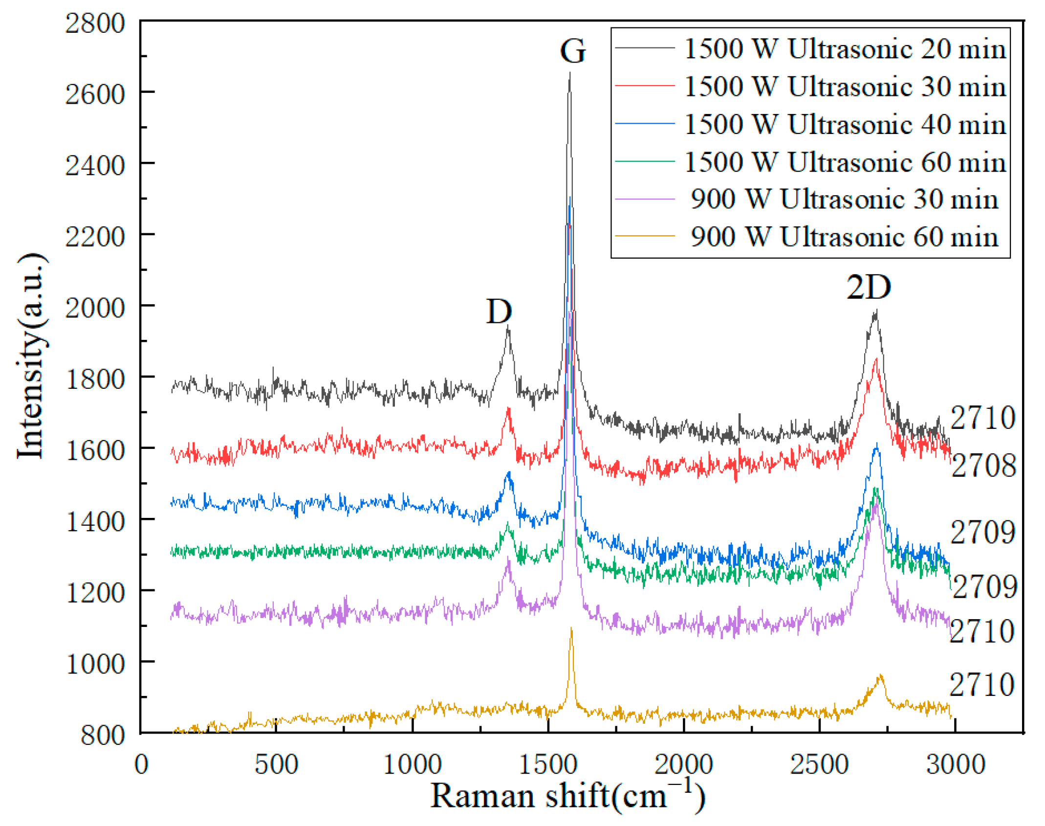
Figure 6.
Transmission electron microscopy results with different process parameters: (a,b) ultrasonic power 1500 W ultrasonication time 30 min, (c,d) ultrasonic power 1500 W ultrasonication time 60 min.
Figure 6.
Transmission electron microscopy results with different process parameters: (a,b) ultrasonic power 1500 W ultrasonication time 30 min, (c,d) ultrasonic power 1500 W ultrasonication time 60 min.


Figure 7.
AFM diagram of graphene on ultrasonic power l500 W and ultrasonication time of 30 min on mica substrate.
Figure 7.
AFM diagram of graphene on ultrasonic power l500 W and ultrasonication time of 30 min on mica substrate.

Figure 8.
Distribution histogram of graphene layers.


Table 1.
Validation data for the concentration formula.
| Dilution Factor | Absorbance | Calculated Concentration (mg/mL) | Actual Concentration (mg/mL) |
|---|---|---|---|
| 50 times | 0.270 | 0.106 | 0.1 |
| 0.272 | 0.107 | ||
| 0.272 | 0.107 | ||
| 60 times | 0.212 | 0.083 | 0.083 |
| 0.214 | 0.084 | ||
| 0.212 | 0.083 | ||
| 100 times | 0.132 | 0.051 | 0.05 |
| 0.130 | 0.050 | ||
| 0.130 | 0.050 |
Table 2.
Range and level of factors.
| Number | Factor Name | Horizontal Code | ||
|---|---|---|---|---|
| −1 | 0 | 1 | ||
| x1 | Ultrasonication time/min | 30 | 90 | 150 |
| x2 | Ultrasonic power/W | 300 | 900 | 1500 |
| x3 | Graphite initial weight/g | 0.5 | 1 | 1.5 |
Table 3.
Box–Behnken d experimental design table.
| Group | Ultrasonication Time/min | Ultrasonic Power/W | Graphite Initial Weight/g | Concentration (mg/mL) | Yield |
|---|---|---|---|---|---|
| 1 | 30 | 300 | 1 | 0.51 | 0.102 |
| 2 | 90 | 300 | 0.5 | 0.46 | 0.184 |
| 3 | 90 | 300 | 1.5 | 0.43 | 0.057 |
| 4 | 150 | 300 | 1 | 0.11 | 0.022 |
| 5 | 30 | 900 | 0.5 | 0.78 | 0.312 |
| 6 | 30 | 900 | 1.5 | 0.82 | 0.109 |
| 7 | 90 | 900 | 1 | 0.41 | 0.082 |
| 8 | 90 | 900 | 1 | 0.56 | 0.112 |
| 9 | 90 | 900 | 1 | 0.57 | 0.114 |
| 10 | 150 | 900 | 0.5 | 0.33 | 0.132 |
| 11 | 150 | 900 | 1.5 | 0.24 | 0.032 |
| 12 | 30 | 1500 | 1 | 0.84 | 0.168 |
| 13 | 90 | 1500 | 0.5 | 0.56 | 0.224 |
| 14 | 90 | 1500 | 1.5 | 0.46 | 0.061 |
| 15 | 150 | 1500 | 1 | 0.21 | 0.042 |
Table 4.
Variance analysis table.
| Model | Projects and Factors | Sum of Squares | df | Mean Square | F Value | p Value Prob > F | Significance |
|---|---|---|---|---|---|---|---|
| Graphene yield | Model | 0.086 | 8 | 0.011 | 52.38 | <0.0001 | Significant |
| x1 | 0.027 | 1 | 0.027 | 130.99 | <0.0001 | ||
| x2 | 0.002 | 1 | 2.1 × 10⁻³ | 10.33 | 0.0183 | ||
| x3 | 0.044 | 1 | 0.044 | 214.87 | <0.0001 | ||
| x1 × x2 | 5.29 × 10⁻⁴ | 1 | 5.29 × 10⁻⁴ | 2.59 | 0.1589 | ||
| x1 × x3 | 2.65 × 10⁻³ | 1 | 2.65 × 10⁻³ | 12.96 | 0.0114 | ||
| x2 × x3 | 3.24 × 10⁻⁴ | 1 | 3.24 × 10⁻⁴ | 1.58 | 0.2550 | ||
| x22 | 1.05 × 10⁻³ | 1 | 1.05 × 10⁻³ | 5.12 | 0.0644 | ||
| x32 | 7.85 × 10⁻³ | 1 | 7.85 × 10⁻³ | 38.35 | 0.0008 | ||
| Lack of fit | 6.7 × 10⁻⁴ | 4 | 1.46 × 10⁻⁴ | 0.45 | 0.7730 | Not Significant |
Table 5.
Concentration and yield of prepared graphene under different process parameters.
| Process Parameters | Average Concentration/(mg/mL) | Yield |
|---|---|---|
| 1500 W and ultrasonication time 20 min | 0.639 | 25.6% |
| 1500 W and ultrasonication time 30 min | 0.790 | 31.6% |
| 1500 W and ultrasonication time 40 min | 0.715 | 28.6% |
| 1500 W and ultrasonication time 60 min | 0.621 | 24.8% |
| 900 W and ultrasonication time 30 min | 0.780 | 31.2% |
| 900 W and ultrasonication time 60 min | 0.599 | 24% |
Table 6.
The main features of Raman spectra obtained for different process parameters. The ID/IG is the peak intensity ratio of the D peak and G peak and the I2D/IG is the peak intensity ratio of the 2D peak and G peak.
Table 6.
The main features of Raman spectra obtained for different process parameters. The ID/IG is the peak intensity ratio of the D peak and G peak and the I2D/IG is the peak intensity ratio of the 2D peak and G peak.
| Process Parameters | Position (cm−1) | Average Value | Average Value | ||
|---|---|---|---|---|---|
| D | G | 2D | ID/IG | I2D/IG | |
| 1500 W and ultrasonication time 20 min | ~1350 | ~1579 | ~2710 | 0.73 | 0.75 |
| 1500 W and ultrasonication time 30 min | ~1350 | ~1578 | ~2709 | 0.77 | 0.83 |
| 1500 W and ultrasonication time 40 min | ~1351 | ~1579 | ~2709 | 0.66 | 0.71 |
| 1500 W and ultrasonication time 60 min | ~1350 | ~1577 | ~2709 | 0.73 | 0.77 |
| 900 W and ultrasonication time 30 min | ~1350 | ~1576 | ~2710 | 0.70 | 0.77 |
| 900 W and ultrasonication time 60 min | ~1351 | ~1576 | ~2710 | 0.72 | 0.78 |
Disclaimer/Publisher’s Note: The statements, opinions and data contained in all publications are solely those of the individual author(s) and contributor(s) and not of MDPI and/or the editor(s). MDPI and/or the editor(s) disclaim responsibility for any injury to people or property resulting from any ideas, methods, instructions or products referred to in the content. |
© 2024 by the authors. Licensee MDPI, Basel, Switzerland. This article is an open access article distributed under the terms and conditions of the Creative Commons Attribution (CC BY) license (https://creativecommons.org/licenses/by/4.0/).
Share and Cite
MDPI and ACS Style
Yi, J.; Gu, B.; Kan, C.; Lv, X.; Wang, Z.; Yang, P.; Zhao, H. Mathematical Model of Graphene Yield in Ultrasonic Preparation. Processes 2024, 12, 674. https://doi.org/10.3390/pr12040674
AMA Style
Yi J, Gu B, Kan C, Lv X, Wang Z, Yang P, Zhao H. Mathematical Model of Graphene Yield in Ultrasonic Preparation. Processes. 2024; 12(4):674. https://doi.org/10.3390/pr12040674
Chicago/Turabian StyleYi, Jinquan, Baoshan Gu, Chengling Kan, Xudong Lv, Zhifeng Wang, Peiyan Yang, and Haoqi Zhao. 2024. "Mathematical Model of Graphene Yield in Ultrasonic Preparation" Processes 12, no. 4: 674. https://doi.org/10.3390/pr12040674
Note that from the first issue of 2016, this journal uses article numbers instead of page numbers. See further details here.