
A Cold Flow Model of Interconnected Slurry Bubble Columns for Sorption-Enhanced Fischer–Tropsch Synthesis


Engler-Bunte-Institute, Karlsruher Institute of Technology (KIT), Engler-Bunte-Ring 1, 76131 Karlsruhe, Germany
*
Author to whom correspondence should be addressed.
ChemEngineering 2024, 8(3), 52; https://doi.org/10.3390/chemengineering8030052
Submission received: 21 March 2024
/
Revised: 23 April 2024
/
Accepted: 6 May 2024
/
Published: 8 May 2024
Abstract
:For technical application with continuous operation of sorption-enhanced (SE) reactions, e.g., Fischer–Tropsch, a special reactor concept is required. SE processes are promising due to the negative effects of water on conversion and catalyst. The reactor concept of two interconnected slurry bubble columns combines the reaction with in situ water removal in the first, and sorbent regeneration in the second column with continuous exchange of slurry between the two. The liquid circulation rate (LCR) between the columns is studied in a cold flow model, measured by an ultrasonic sensor. The effects of different operating and geometric parameters, e.g., superficial gas velocity, liquid level and tube diameter on gas holdup and LCR are discussed and modelled via artificial intelligence methods, i.e., extremely randomized trees and neural networks. It was found that the LCR strongly depends on the gas holdup. The maximum of 4.28 L min−1 was reached with the highest exit, widest tube and highest superficial gas velocity of 0.15 m s−1. The influence of liquid level above the exit was marginal but water quality has to be considered. Both models offer predictions of the LCR with errors < 6%. With an extension of the models, particle circulation can be studied in the future.
1. Introduction
In recent years, there has been increasing interest in sorption-enhanced (SE) processes, particularly when water is produced as an undesired by-product, as seen in Fischer–Tropsch (FT) synthesis, methanation or dimethyl ether synthesis [1,2,3]. FT synthesis, in particular, has garnered attention due to its potential for producing carbon-neutral energy carriers from various feedstocks such as biomass or plastic waste in combination with renewable energy. FT synthesis is the key technology in power-to-liquid (PtL) processes, converting synthesis gas (a mixture of CO and H2) into a broad spectrum of liquid hydrocarbons (-CH2-). The FT reaction
is an exothermic polymerization reaction with a large equilibrium constant of Keq (250 °C, H2 and CO to C6H14) 1·1020. This implies that the FT reaction is not controlled by the equilibrium [1]. When using Fe-based catalysts, the water–gas-shift (WGS) reaction occurs as the main side reaction of FT synthesis. The WGS reaction
is an equilibrium limited reaction. The removal of water leads to an equilibrium shift towards the production of CO, subsequently enhancing the conversion to long-chain hydrocarbons, which is desirable in PtL processes. In the case of the FT reaction, where the impact of equilibrium displacement is negligible, other factors, such as kinetic inhibition and catalyst deactivation, become relevant. Various effects, which depend on the amount of added or indigenous water, as well as the support materials of the catalyst, are reported in the literature [4,5,6,7]. Jacobs et al. [4] claimed that water acts as a kinetic inhibitor at low water partial pressures due to the adsorption of water molecules at the active sites of the catalyst. High water partial pressures of added water above 25% lead to a deactivation of the catalyst by changing the catalyst’s structure [4,5]. Moreover, Li et al. [5] claimed that high water partial pressures deactivate the catalyst permanently. However, Storsater et al. [6] found that the support material of the catalyst makes a difference in catalyst activity. Adding more than 20% water to the feed increases the activity of TiO2-supported catalysts, but the opposite behavior was observed with SiO2-supported catalysts. Krishnamoorthy et al. [7] investigated an increase in CO conversion and C5+ selectivity with increasing H2O concentration to a constant level at 0.8 MPa H2O with SiO2-supported catalysts. Bartholomew et al. [8] summarized that the main reason for deactivation is due to the formation of oxides and inactive Co-supported spinel compounds, which is accelerated at high water partial pressures (>0.5–0.6 MPa). These partial pressures are easily archived at moderate CO conversions (>60%). The benefits of in situ water removal during FT synthesis were outlined by Rohde et al. [9], while a recent investigation by Gavrilovic et al. [10] demonstrated increased CO conversion using zeolite 13X in FT synthesis within a fixed bed reactor. Nevertheless, it is evident that additional research examining the impact of water is needed in future studies.
Considering the aforementioned negative effects of water, this publication primarily focuses on a new reactor concept for SE FT synthesis. The concept involves the in situ removal of water from the reaction zone due to adding commercially available water sorbents, i.e., zeolites. Zeolite 13X has already demonstrated excellent performance in SE processes due to larger pores and higher adsorption capacities at elevated temperatures [2,10,11,12,13]. However, adsorption isotherms at relevant FT conditions are rare in the literature. Even less information is available about adsorption capacities in a three-phase system, which should be the focus of further studies on three-phase SE FT.
The investigated reactor concept in this work combines two slurry bubble columns (SBCs). SBCs are the preferred reactor type in commercial large-scale three-phase FT plants due to the well-mixed liquid phase, resulting in nearly isothermal operation. Additional benefits include low complexity and the possibility of easy catalyst replacement during operation [14,15,16,17]. The slurry, consisting of the liquid FT product and catalyst, is sparged with synthesis gas at the bottom of the column, expanding the slurry as soon as the gas is introduced. Relative gas holdup (), a significant operation and scale-up parameter, is defined in Equation (3) as the volume of the gas phase () divided by the sum of gas volume, particle volume () and liquid volume ().
Gas holdup depends on various parameters, which are partly addressed in this publication, such as injected gas volume flow, degree of ionization, particle size and concentration, column diameter and gas distributor. Depending on these parameters, different regimes arise inside the columns. Typically, FT synthesis is carried out in the heterogenous regime, providing good heat and mass transfer.
To combine the FT reaction with in situ water removal, sorbent regeneration must be provided when the sorbent is saturated with water. For continuous operation of the reaction, water adsorption and desorption, a new reactor concept of two interconnected SBCs was developed, as shown in Figure 1. The slurry consists of the reaction product, namely the liquid FT product (and water), and the solid particles, namely the catalyst and sorbent material. In one of the two SBCs, the middle distillates (and water) are synthetized from synthesis gas, while the sorbent material removes the water produced. The catalyst and sorbent material enter the second column via the looping liquid FT product, where the desorption takes place. The principle of the circulation is based on density differences of the slurry and is commonly used in airlift reactors [18].
This work focuses on fundamental research on a new reactor concept, utilizing a cold model of interconnected slurry bubble columns to investigate principal hydrodynamics and circulation rates. In the initial phase, a water–air system is considered. Currently, only one publication addresses a similar reactor concept. Jafarian et al. [19] introduced a cold model of interconnected bubble columns (BC) with an identical column diameter of 85 mm and successfully demonstrated the concept of circulating liquid. They observed an impact of injected gas flow and unaerated liquid height on the liquid circulation but found barely any influence of the aeration nozzle diameter. However, to gain a more precise understanding of this reactor concept, further influences, i.e., diameter of the loop, liquid exit height () and properties of the liquid, need to be studied, and these are addressed in this work. In the context of SE FT synthesis, sorbent particles require different residence times in the columns because desorption is the time-limiting step. This can be achieved with different column diameters and bubble regimes in each column, which is part of this work. To enable liquid circulation, gas separators at the liquid exits are necessary. In this publication, gas separators are designed to enable slurry circulation unlike in Jafarian et al.’s work [19], which is only suitable for gas–liquid separation.
Airlift reactors are found in various configurations, e.g., external or internal loop, sharing the common feature of gas injection at the bottom of the riser, leading to the circulation of liquid or slurry due to hydrostatic pressure differences between riser and downcomer [18]. Numerous publications have addressed the prediction of liquid velocity and gas holdup, considered as the most relevant parameters for reactor characterization and scale-up. Many of these models are based on the procedure developed by Hsu and Dudukovic [20]. An overall momentum balance for the loop is employed, assuming that during steady-state operation, the hydrostatic pressure difference must equal the pressure drop in the downcomer and riser. Several authors [21,22,23] have extended the model by incorporating the two-phase drift-model of Zuber and Findlay [24] or by using an energy balance instead [25,26]. Depending on the complexity of the models, different agreements between the model and experiments have been achieved (ranging from 5% [21] to approximately 20% [23] error on liquid velocity). Jafarian et al. [19] established an empirical correlation for predicting the liquid circulation rate (LCR) between the two bubble columns within 15%, except for two data points. However, it is important to note that this correlation is only valid for the specific experimental setup and is not transferable to other reactor configurations.
In the present work, an alternative approach is introduced for predicting the LCR using artificial intelligence (AI) methods. Several models have been reported for determining gas holdup in (slurry) bubble columns through the application of artificial neural networks (ANN). Over the years, ANN models have demonstrated the capability to predict a wide range of data with a regression coefficient (R2) 0.9 [27,28,29,30]. Behkish et al. [29] developed an ANN, which is capable of predicting synthesis gas holdup depending on different operating conditions during FT synthesis, e.g., temperature, pressure and catalyst loading with a R2 of 0.93. Hazare et al. [31] compared various AI methods, i.e., ANN, random forest, support vector regression and extra trees regressor (EXT) and demonstrated the superior performance of the latter with a mean absolute percentage error (MAPE) < 8%. Therefore, in this work, an ANN and an EXT model for predicting the LCR are presented and compared in terms of prediction accuracy, runtime and complexity.
2. Materials, Methods and Methodology
2.1. Experimental Setup and Measuring Methods
The experiments are conducted in a cold model of the novel reactor concept. The reactor consists of two interconnected slurry bubble columns (Figure 2). The gas separators (GS) are designed as funnels, enabling slurry to circulate from one column to the other column without sedimentation of the particles. However, in this work, only a water–air system is used to proof the concept and indicate the most significant influences on liquid circulation, which will be extended to particle circulation in the future. The plexiglass columns have an inside diameter of 100 mm (BC1) and 140 mm (BC2) with an identical height of 1.5 m. Three liquid exits can be used at different heights along the columns (see Figure 2). For liquid fluidization, two sintered metal plates with pore diameters of 5 μm are used in both columns.
The superficial gas velocity () is calculated as the gas volume flow () divided by the cross-sectional area of one BC (), as deduced in Equation (4). In this work, the superficial gas velocity is varied from 0.01 m s−1 to 0.15 m s−1, covering homogenous, transition and heterogenous bubble flow regime.
The gas volume flow is controlled by two mass flow controllers (MFC), one per column, allowing operation with different superficial gas velocities in each column. Filtered and pressurized air is used for the fluidization of water. The degree of ionization of the water is measured and serves as an indicator of water quality. It is determined with an electrical conductivity measuring device from Mettler Toledo. The electrical conductivity of the water () is varied from 1 to 750 μS cm−1. Experiments are carried out at ambient pressure and temperature, with temperatures ranging from 15 to 21 °C, and the pressure varying from 998 to 1013 mbar.
The manometric method [32] is employed for measuring relative gas holdup. By neglecting wall friction and the acceleration contribution in the momentum balance, the gas holdup can be calculated using Equation (5). Another assumption is a negligibly small gas density compared to liquid density ().
In Equation (5), the acceleration due to gravity (g) and the difference in static pressure with () and without fluidization () between two sensors placed at a distance () are used. Pressure measurements are performed with pressure transmitters (Type A-10, 0–200 mbar, WIKA). All measured values are recorded in five-second intervals with a programmable logic controller (PLC). The standard deviation of gas holdup ( is calculated using the Gaussian error propagation. By differentiating the variables ( and ) and multiplying with the standard deviation of the differential pressures with and without aeration ( and ), the following Equation (6) is derived.
The standard deviation is calculated for each measuring point and presented as error bars in all figures.
LCR () is measured with an ultrasonic clamp-on flow meter (Sonoflow CO.55/160, SONOTEC). The position of the sensor can be seen in Figure 2 (indicated with FI). Barely any influence was detected by changing the sensor’s position along the tubes. The non-invasive measuring principle is based on the transit-time method (Figure 3). The time difference between the time of flight of the ultrasonic wave with and against the liquid’s flow direction is a measure for the fluid velocity. Multiplying the velocity with the cross-sectional tube area allows determining the LCR. The connecting PVC tubes can be changed, except for the tube on which the flow meter is fixed (15 mm). The tube inner diameter () in this work is varied from 10 to 15 mm. For reproducibility, two reference points are tested before running a new measurement series. The deviation of the reference points is <2% and within the measuring error of the ultrasonic flow sensor (see Appendix A).
The liquid level () is measured in each column using two top-mounted level indicators (Type UTN, WIKA; indicated with LI in Figure 2) with a measuring uncertainty of ±5 mm.
2.2. AI Modelling
This section outlines the general procedure for predicting LCR using supervised machine learning algorithms. The flow chart in Figure 4 provides a general overview of the modelling process, which is divided into three main parts.
- Preprocessing: This step involves extracting, cleaning and separating the experimental data, which is comprised of 95 data points. The data are divided into features and labels. In this work, the features include gas volume flow in both BC, liquid exit height, tube inner diameter and electrical conductivity. Since only LCR is supposed to be predicted, the number of labels is one.
- All features are normalized with a MinMaxScaler from sklearn within the interval [0, 1], using Equation (7). This procedure is essential to avoid any potential influence of the differing value ranges of the features. Each normalized value of a feature ) is calculated using its maximum () and minimum () values alongside the actual value ().
- 3.
- This equation is suitable as it retains the relative scaling between all feature values. The last step of preprocessing involves splitting the data into training and testing data. Typically, 70–80% of the original data are used for training, while the remaining 20–30% are reserved for evaluating model’s accuracy [27].
- 4.
- Training: In this step, the models are trained. A multilayer perceptron (MLP) and EXT model are developed in the present work. Both are explained in greater detail in Section 2.2.1 and Section 2.2.2. Identical training data are supplied to both models and optimal hyperparameters (HPs) are determined using the GridSearchCV method from sklearn. This method has the option of performing a k-fold cross-validation to enhance the model’s accuracy. In this work, a 5-fold cross-validation is performed for each fit in the gird search algorithm. Defined HPs and their ranges for both models are listed in Table 1 and Table 2. Both models are optimized with the mean squared error (MSE) as presented in Equation (8).
- 5.
- MSE is defined as the sum of squared differences between the experimental value () and the predicted value () for n predictions. The fits with the lowest MSE are used in the following step. Parity plots of the training data are plotted with matplotlib.
- 6.
- Testing and Evaluation: In this step, the remaining unknown testing data are used to assess the model’s accuracy. Parity plots are generated using matplotlib. For comparison, MAPE and R2 are calculated and saved. MAPE is defined as the sum of differences between the experimental value () and the predicted value () divided by the experimental value for n predictions (Equation (9)).
- 7.
- R2 is defined as the sum of residual squares divided by the total sum of squares (Equation (10)). The sum of residual squares is calculated by the sum of squared differences between the experimental () and predicted value . The sum of total squares contains the sum of squared differences between the experimental value () and the mean experimental value .
- The closer the value of is to one, the better the predicted data represent the experimental values. All models, along with the best HPs, are saved using joblib.
2.2.1. Multilayer Perceptron
ANN are popularly used as universal approximators for complex data due to their ability to accurately predict non-linear relationships between dependent and independent data [33]. Notable ANN structures include single-layer feed-forward, feed-backward, or multilayer feed-forward networks. The present work deals with a regression problem, making the multilayer-feed-forward network a suitable candidate. In Figure 5, the structure of this specific type of ANN is presented. It consists of one input and output layer, separated by an arbitrary number of hidden layers.
Each layer is composed of neurons. The number of neurons in the input and output layer corresponds to the given number of features and labels, respectively. Each neuron n in hidden layer m contains a certain value (). All neurons of one hidden layer are connected to the neurons of the following layer, with each connection represented by a weight. The weights are adapted via backpropagation during training to improve the model’s accuracy. In this work, the MLPRegressor from sklearn is used.
Table 1 presents all optimized HPs, their range, and the final value found by GridSearchCV. The selected batch size, number of neurons per hidden layer and learning rate fall within the given HP range. The chosen and expected activation function is the rectified linear unit (ReLU) function, given that labels are within the range of 0 < < 4.5 L min−1. ReLU is particularly suitable for dealing with values lager than one. Notably, for both the number of hidden layers and the number of epochs the maximum values were selected. This implies that a further expansion of the HP range in the grid search algorithm could potentially improve the model’s accuracy. However, a broader range of HPs would increase the required computational resources. Thus, a further increase in range limits was not performed.

Table 1.
Optimized hyperparameters, range and final value using GridSearchCV for MLP.
| Hyperparameter | Range | Final Hyperparameter |
|---|---|---|
| Batch size | 5, 10, 20 | 10 |
| Number of hidden layers | 1, 2, 3 | 3 |
| Number of neurons | 8, 16, 64, 128, 512 | 128 |
| Number of epochs | 100, 300, 500, 1000, 1500 | 1500 |
| Learning rate | 10−4, 10−3, 10−2 | 10−3 |
| Activation function | Rectified linear unit, hyperbolic tangent, sigmoid | Rectified linear unit |
2.2.2. Extra Trees
EXT is an ensemble machine learning method based on a decision tree algorithm. In ensemble machine learning methods, multiple models are developed simultaneously. By combining all model results, an accurate estimation can be achieved. EXT belongs to the family of bagging methods, which is a subclass of ensemble methods that relies on a two-step process. In the first step, known as bootstrap, data are split into n datasets. Typically, EXT methods randomly shuffle the data in each of these datasets. With each dataset, a decision tree is developed. The aggregation step involves combining the predictions of all decision trees to obtain a final prediction. Schematically, the bagging method is presented in Figure 6, including both the bootstrap and aggregation step.
In general, a decision tree consists of four types of nodes: one root node, parent nodes, child nodes and leaf nodes [34]. In the root node and each parent node, data are split depending on a threshold, selected from the range of values for one feature. This process of splitting data is repeated in every parent node. Nodes that are placed below the root node or parent nodes are called child nodes. Based on mathematical criteria or user-based input, the separation into further child nodes is stopped. These nodes are known as leaf nodes. They do not have any further downward connection and return a prediction value. Finally, in the aggregation step the predictions of every developed tree are combined into one mean prediction. Sklearn provides an EXTRegressor method, which is used in this work. Table 2 presents all optimized HPs, their range and the final value for the models using GridSearchCV by sklearn.
Table 2.
Optimized hyperparameters, range and final value using GridSearchCV for EXT.
| Hyperparameter | Range | Final Hyperparameter |
|---|---|---|
| n_estimators | 10, 50, 100, 200, 500 | 100 |
| max_depth | None, 5, 10, 20, 30 | 5 |
| max_features | None, 2, sqrt, log2, 0.3 | None |
| min_sample_split | 5, 10, 20 | 5 |
The HPsn_estimators and max_depth control the number of estimators and the maximum depth of any tree, respectively. The final values for both are chosen within the given HP range. The HP max_features determines the number of features supplied to a given tree. The selected default value None implies that every feature is considered in the trees. The parameter min_sample_split regulates how many data points are allowed to remain in one leaf of the tree, at which point further separation is stopped.
3. Results and Discussion
3.1. Cold Model Studies
3.1.1. Effect of Superficial Gas Velocity on LCR
Figure 7 illustrates the dependence of gas holdup and LCR on the superficial gas velocity, which is equal in both columns. At low superficial gas velocities ( < 0.05 m s−1), a linear correlation between gas holdup and is observed. At higher gas velocities, the linear character disappears, and a local maximum arises until the gas holdup remains constant with increasing gas velocities for > 0.09 m s−1 within the standard deviation. This behavior indicates the formation of homogenous, transition and heterogenous flow regime, similar to conventional bubble columns using sintered metal plates as gas distributor [35]. Throughout all experiments, a slightly higher gas holdup was measured in BC2. Reports in the literature about the impact of column diameter on gas holdup are contradictory, including no influence of column diameter or a lower gas holdup with increasing column diameter [35,36]. However, comparisons were mainly made between large column diameters. Due to the small diameter of BC1 (100 mm), wall effects become more relevant, and slug flow has to be taken into account at elevated gas velocities, resulting in lower gas holdups due the formation of large, slug shaped bubbles [37].
The main driving force of liquid circulation between the columns is a result of the hydrostatic pressure differences in the aerated bubble columns and unaerated connection tubes. This principle is comparable to an airlift reactor, where each BC serves as riser and the connection tubes serve as downcomers. A strong dependency of the gas holdup on the LCR is observed in Figure 7, resulting from density differences due to aeration of the BC. Equation (11) shows the correlation between the density of the liquid phase in the aerated bubble columns () and gas holdup.
For the reactor configuration in this work, the lowest LCR was 1.8 L min−1 for the lowest superficial gas velocity ( = 0.02 m s−1), while it was 4.28 L min−1 at the highest ( = 0.15 m s−1). These values are higher than the observed ones from Jafarian et al. [19] because of the larger column height, as well as column and tube diameters used in this work. For a stable circulation, a minimum superficial gas velocity of = 0.015 m s−1 is necessary; otherwise, the density differences and total energy input through the injected gas flow are not sufficient, and bubbles rise inside the tubes against the flow direction.
For the experiments in Figure 7, a constant liquid exit height ( = 800 mm), liquid level ( = 900 mm), tube inner diameter ( = 15 mm) and electrical conductivity = 250 μS cm−1) were used.
3.1.2. Effect of Water Quality and Liquid Height on LCR
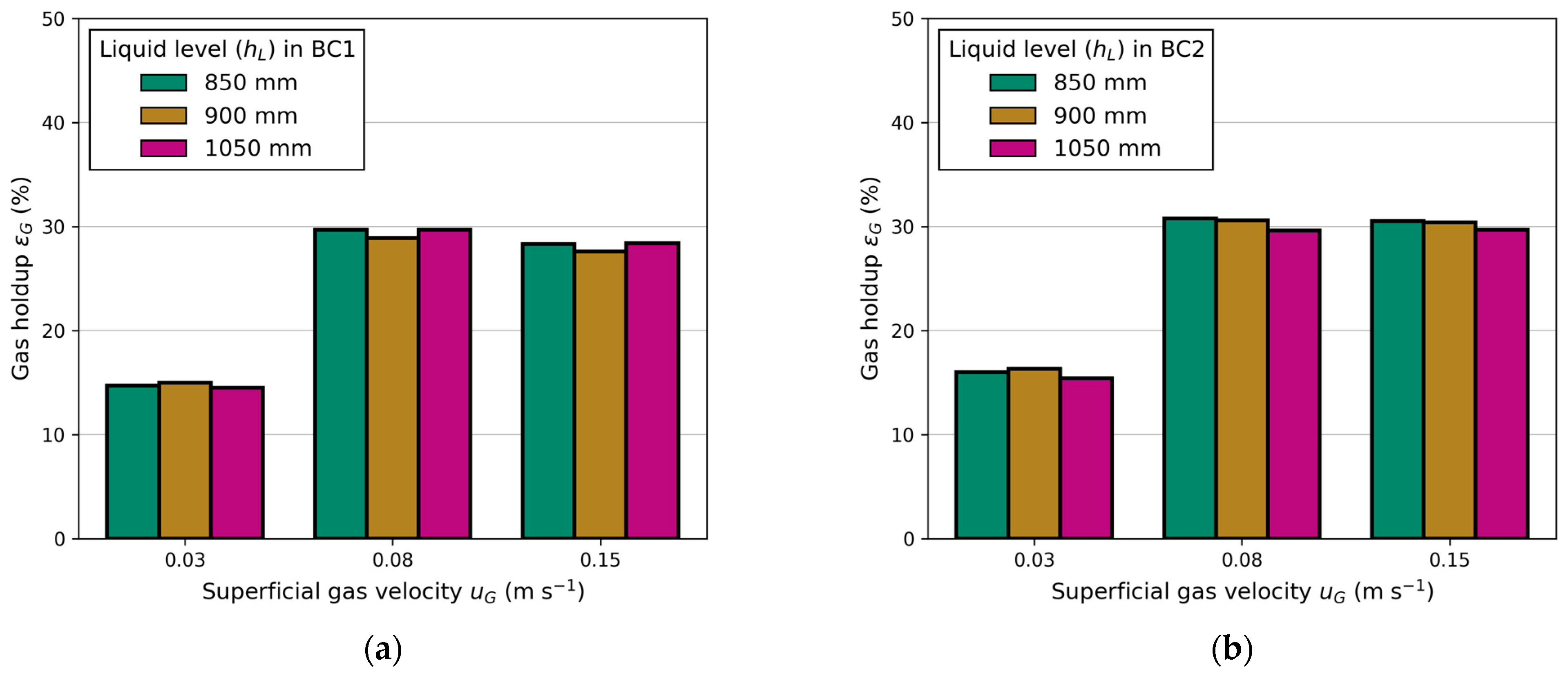
Figure 8 presents a comparison of the measured LCR between the columns, considering variations in electrical conductivity and different liquid levels above the exits. Both the superficial gas velocity and liquid level are adjusted equally in each column. Figure 8a shows barely any influence of the liquid level on the LCR. This outcome was expected due to constant gas holdup and equal aeration (see Appendix B).
Figure 8b demonstrates the impact of electrical conductivity, a measure of water quality. The comparison is made between fully demineralized water ( = 1–2 μS cm−1) and laboratory water ( = 250 μS cm−1). Measuring electrical conductivity involves applying a voltage between two electrodes. The drop in voltage due to the resistance of water is used to measure the water’s conductivity. Fully demineralized water, containing fewer particles, exhibits a lower drop in voltage compared to contaminated laboratory water. A higher particle concentration in the water suppresses bubble coalescence, explaining the higher gas holdups in BC1 and BC2 (Figure 9a,b) when using water with high electrical conductivity. Reports in the literature regarding water quality and its influence on gas holdup in conventional BC are scarce. However, Gemello et al. [38] demonstrated similar results by comparing demineralized and tap water. The slightly higher gas holdup of tap water is explained by contaminants suppressing bubble coalescence, leading to a decrease in mean bubble size [38]. The differences in gas holdup between BC1 and BC2 (shown in Figure 9) are due to the distinct column diameters, as discussed previously. For elevated gas velocities, the standard deviation increases due to recirculating bubbles, causing deviations in pressure measurements. In general, for any given experiments, a higher electrical conductivity leads to an equal or higher gas holdup. This trend is propagated to LCR, which exhibits a similar progression, due to its proportionality to gas holdup (Figure 8b).
3.1.3. Effect of Liquid Exit Height and Tube Diameter on LCR
Figure 10 illustrates the LCR as a function of the superficial gas velocity for various tube inner diameters and liquid exit heights. The observed trend indicates an increase in LCR with higher liquid exits (Figure 10a). These observations are consistent with those made by Jafarian et al. [19] and in conventional airlift reactors [25,39]. However, it is noteworthy that Jafarian et al. [19] used a maximum liquid exit height of 600 mm, while the liquid exit height varies from 400 to 800 mm in this work. At the same exit height ( = 600 mm) and superficial gas velocity ( = 0.15 m s−1), the maximum LCR in this work is 1.5-fold higher compared to Jafarian et al. [19]. The primary factor contributing to this observation is the lower gas holdup, which is approximately 14% compared to 25% in this work. The reduction is attributed to the smaller column size and utilization of different gas distributors (injection nozzles compared to sintered metal plates). Another reason might be the use of smaller tube sizes, as elaborated upon in the following section.
The tube inner diameter influences the LCR, as presented in Figure 10b. The measured LCR increases with higher superficial gas velocity and tube inner diameter. Once again, LCR demonstrates proportionality to gas holdup, but higher LCR can be achieved with a larger tube inner diameter. This observation is comparable to studies on the ratio of the downcomer-to-riser cross-sectional area in conventional airlift reactors. The significance of this ratio was highlighted by Chisti et al. [25,32], who observed a similar trend. Gavrilescu and Tudose [40] stressed that this ratio is the principal factor, which controls the friction, resulting in a higher pressure drop with a smaller downcomer (tube) cross-sectional area. For a tube inner diameter of = 10 mm, no stable circulation could be achieved, as indicated by rising bubbles inside the tubes in the opposite flow direction. Therefore, only two measuring points were carried out at = 0.03 m s−1 and 0.06 m s−1. Instable or non-reproducible data points are excluded in the subsequent modelling process.
3.1.4. Identifying the Main Influencing Parameter on LCR for SE FT Synthesis
Gas holdup in BC1 and BC2 are identified as the primary influencing parameters on LCR, alongside geometric parameters, i.e., liquid exit height and the ratio of tube-to-column cross-sectional area. Variations in superficial gas velocity and electrical conductivity result in changes in gas holdup, thereby affecting LCR. The influence on gas holdup is more dominant than the total energy input through the injected gas flow, as indicated by a higher LCR at higher gas holdups but lower total gas volume flow (Figure 11). Liquid level shows barely any influence on gas holdup and LCR. In addition to gas holdup, the geometry of the reactor must be considered. Liquid exit height and tube inner diameter both affect LCR. These observations are summarized in Figure 11, which depicts the dependency of LCR on total gas holdup () and total gas volume flow (). The total variables are each made up of the respective ones in BC1 and BC2. A nearly linear correlation between LCR and total gas holdup can be seen for one reactor configuration. With changing geometric parameters of the reactor, different magnitudes of LRC can be achieved. To underline the results from Figure 11, the Pearson correlation coefficients for LCR and all varied parameters can be found in Appendix C. This information gain is valuable for developing a reactor configuration for chemical processes, such as SE FT synthesis, when the necessary residence times in the columns are known.
For SE FT synthesis, residence times for the FT reaction, adsorption and desorption in both columns have to be specified. With the knowledge of the necessary residence times, columns diameter and the circulation rate, particularly the particle circulation rate can be determined. For SE FT synthesis, it depends on different factors, e.g., sorbent to catalyst ratio, ad- and desorption kinetics of water sorbents at FT conditions as well as FT catalyst, kinetics and feed ratio. Although the literature reports in the field of ad- and desorption kinetics of sorbents at FT condition and SE FT reaction kinetics are currently limited, further studies are needed. However, with the assumption of 30 wt.% particles in the slurry, typical for FT SBCs [41], and an appropriate catalyst to sorbent ratio of 1:2, the necessary circulation rate until the sorbent is fully saturated is far below the specified LCR achieved in this work. Adsorption kinetics taken from Ghodhbene et al. [13] for zeolite 13X at 250 °C and FT kinetics from Zimmerman and Bukur [42] for an Fe-based catalyst in a slurry reactor were used for estimation. It demonstrates the suitability of the new reactor concept for SE FT synthesis and indicates sorbent and catalyst performance as potential bottlenecks. Since desorption takes longer than adsorption, the residence time in the regeneration column must be longer than in the adsorption column. This can be achieved by using different column diameters, as presented in this work. The liquid residence time in BC2 is 1.96-fold higher than in BC1. Optimal residence times depend on ad- and desorption kinetics and can be adapted with the column diameter ratio. Nevertheless, the particle circulation rate in the new reactor concept requires further investigations in the future.
3.2. AI Modelling
As mentioned in Section 2.2, the models aim to predict a single label, namely the LCR, using multiple features. A total of 95 data points were used to train and test the models. In order to compare the models, MAPE and R2 were calculated for both the training and testing datasets. The results for MLP and EXT models are listed in Table 3.
Considering the training data, it can be observed that the EXT model exhibits more accurate predictive capabilities with a MAPE of 1.1% compared to the MLP model, which has a MAPE of 3.4%. The EXT model achieved a high R2 of 0.99, accurately representing the original experimental data. On the other hand, the MLP model shows a lower adaption with an R2 of 0.96. Furthermore, when comparing the models in terms of training runtime, it is evident that the MLP model’s training is significantly slower. While the EXT model completes the HP tuning within 60 s, the MLP model takes over 9000 s. The exact runtime of the models depends on various factors, including the provided data, the HP ranges, and the processing performance of the executing computer (more information in Appendix D). However, a similar trend in runtime efficiency was observed by Hazare et al. [31,43]. The computational effort is reduced once the trained models are used for making predictions. Nevertheless, it should be considered during possible retraining, when adapting to new data or adding new labels. The predictions with testing data reveal that the EXT model can more accurately predict previously unknown data, with a MAPE of 4.5%. Again, the MLP model is less accurate with a MAPE of over 5%. Typically, when predicting gas holdup in conventional BC with AI models, large datasets of up to 5000 datapoints are supplied. However, our models proved that for this application, a dataset of <100 data points is sufficient to accurately predict the LCR. In Appendix E, the influence of available data is presented.
The parity plots shown in Figure 12 include both training and testing data, as well as ±10% bounds to indicate accurate predictions. Predictions within these bounds deviate less than 10% from the actual data. The data predominantly consist of tube inner diameter of 15 mm, liquid exit height of 800 mm, and electrical conductivity of 250 μS cm−1. A detailed overview of the used feature and label values can be found in Appendix D. Consequently, the models should accurately predict the LCR for this configuration. The parity plots of the EXT model are displayed in Figure 12a. Regardless of the reactor configuration, the EXT model accurately predicts the LCR. It is worth noting that even the underrepresented data, such as varying liquid exit heights and tube inner diameters, are predicted with a mean deviation of less than 4.5%. One prediction slightly exceeds the bounds, with a maximum deviation of 12.1% (data point 86 in Table A3, Appendix D). Aside from that, all other data points (training or testing data) are predicted with a deviation <10%. In comparison, Figure 12b shows the predictions of the MLP model. The parity plot exhibits more deviations from the axis bisector, and the MLP predicted four data points with an error of >10%. Notably, these over- and underpredictions occur at the superficial gas velocities that are least represented in the training data, highlighting the need for a more even representation in the supplied dataset. Generally, most predictions fall within the given bounds. This result aligns with earlier investigations of Hazare et al. [31], who conducted a study dealing with the prediction of gas holdup. They found that an EXT model predicted the data more closely compared to a MLP model, resulting in similar parity plots.
In future works, both models will be expanded to predict multiple labels, e.g., gas holdup in both columns and the particle circulation rate. For the latter, further experiments need to be conducted in order to provide a balanced training dataset.
4. Conclusions
A new reactor concept for sorption-enhanced Fischer–Tropsch synthesis, comprising two interconnected slurry bubble columns, was introduced. A cold model for circulating slurry was designed, incorporating gas separators to facilitate continuous slurry circulation, which is advantageous for chemical reactions requiring constant catalyst or sorbent regeneration. Initial studies using a water–air system demonstrated a maximum liquid circulation rate of 4.28 L min−1. The new reactor concept shows similar patterns to conventional airlift reactors in terms of the correlation between the liquid circulation rate, gas holdup, and geometric parameters. This study revealed that LCR strongly depends on total gas holdup, as the circulation is mainly driven by density differences resulting from aeration. Additionally, significant influences on LCR were identified in form of geometric parameters, specifically liquid exit height and the ratio of tube-to-column cross-sectional area. Within a given reactor configuration, the dependency of LCR on gas holdup was found to be nearly linear. In order to operate SE FT synthesis in the new reactor concept, an initial estimation demonstrated the suitability of the new concept by achieving the necessary circulation rate. Nevertheless, further investigations are required, focusing on the particle circulation rate, as well as sorbent and catalyst kinetics under relevant conditions.
Using the experimental data, two AI models, namely a multilayer perceptron and an extra trees model, were developed, trained and tested. The dataset comprised 95 data points with varying gas volume flows in BC1 and BC2, electrical conductivities, liquid exit heights, and tube inner diameters. Both models accurately predicted the LCR, with the extra trees model displaying a better performance, indicated by a slightly lower MAPE and higher R2. The grid search for hyperparameter tuning, including a 5-fold cross-validation, was notably faster while developing the extra trees model. The higher accuracy and faster training runtime suggest that the extra trees model is more suitable for future extensions, such as predicting gas holdup and the particle circulation rate. These extensions require further experiments to provide an adequate training dataset.
Author Contributions
Conceptualization, W.A.; methodology, W.A.; software, R.L.; validation, W.A. and R.L.; formal analysis, W.A. and R.L.; investigation, W.A. and R.L.; resources, W.A. and R.R.; data curation, W.A. and R.L.; writing—original draft preparation, W.A. and R.L.; writing—review and editing, W.A.; visualization, W.A.; supervision, R.R.; project administration, R.R.; funding acquisition, R.R. All authors have read and agreed to the published version of the manuscript.
Funding
This research received no external funding.
Data Availability Statement
The data presented in this study are available on request from the corresponding author. The data are not publicly available due to the value of further research.
Conflicts of Interest
The authors declare no conflicts of interest.
Appendix A
Table A1.
Runtime and standard deviation of reference points.
| Reference Point (m s−1) | Run Time (h) | LCR (L min−1) | Standard Deviation of Reference Points (L min−1) |
|---|---|---|---|
| 0.03 | 20 | 2.68 ± 0.04 | 0.04 |
| 3 | 2.7 ± 0.05 | ||
| 8 | 2.7 ± 0.05 | ||
| 0.06 | 14 | 3.64 ± 0.14 | 0.04 |
| 2 | 3.6 ± 0.15 | ||
| 6 | 3.68 ± 0.15 |
Appendix B
Figure A1.
Influence of liquid level () on gas holdup () at different superficial gas velocities (): (a) in BC 1 and (b) in BC2.
Figure A1.
Influence of liquid level () on gas holdup () at different superficial gas velocities (): (a) in BC 1 and (b) in BC2.
Appendix C
Table A2 shows the Pearson correlation coefficients for LCR and the varying parameters from Section 3.1. It underlines the strong correlation between LCR and total gas holdup as well as liquid exit height. Nearly any correlation was found between LCR and liquid level.
Table A2.
The Pearson correlation coefficients for LRC and different parameters.
| LCR | |||||||
|---|---|---|---|---|---|---|---|
| Correlation coefficient for LCR (-) | 0.176 | 0.91 | 0.002 | 0.178 | 0.485 | 0.908 | 1 |
Appendix D
The hardware used for this study comprised an AMD 16-core 3.4 GHz processor and 32 GB of Corsair DDR4 RAM. All code was developed using Python, version 3.12.
Table A3.
Training and testing data, divided into features and label.
| Features | Label | |||||
|---|---|---|---|---|---|---|
| Index * | Gas Volume Flow BC1 (m3 h−1) | Gas Volume Flow BC2 (m3 h−1) | Liquid Exit Height (mm) | Tube Inner Diameter (mm) | Electrical Conductivity (μS cm−1) | LCR (mL min−1) |
| 1 | 1.70 | 3.33 | 800 | 15 | 250 | 3608.533 |
| 2 | 0.85 | 1.66 | 800 | 15 | 250 | 2686.062 |
| 3 | 1.70 | 3.33 | 800 | 15 | 250 | 3639.435 |
| 4 | 0.85 | 1.66 | 800 | 15 | 250 | 2716.402 |
| 5 | 1.70 | 3.33 | 800 | 15 | 250 | 3652.783 |
| 6 | 0.85 | 1.66 | 800 | 15 | 250 | 2720.485 |
| 7 | 1.70 | 3.33 | 800 | 15 | 250 | 3642.520 |
| 8 | 0.85 | 1.66 | 800 | 15 | 250 | 2688.969 |
| 9 | 1.70 | 3.33 | 800 | 15 | 250 | 3763.355 |
| 10 | 0.85 | 1.66 | 800 | 15 | 250 | 2733.940 |
| 11 | 1.70 | 3.33 | 800 | 15 | 250 | 3786.024 |
| 12 | 2.26 | 4.43 | 800 | 15 | 250 | 4045.343 |
| 13 | 2.26 | 4.43 | 800 | 15 | 250 | 4156.077 |
| 14 | 0.85 | 1.66 | 800 | 15 | 250 | 2680.508 |
| 15 | 2.26 | 4.43 | 800 | 15 | 250 | 4092.790 |
| 16 | 1.13 | 2.22 | 800 | 15 | 250 | 2854.361 |
| 17 | 1.70 | 3.33 | 800 | 15 | 250 | 3640.642 |
| 18 | 0.85 | 1.66 | 800 | 15 | 250 | 2695.432 |
| 19 | 1.41 | 2.77 | 800 | 15 | 250 | 3243.155 |
| 20 | 1.98 | 3.88 | 800 | 15 | 250 | 3744.599 |
| 21 | 2.54 | 4.99 | 800 | 15 | 250 | 3893.254 |
| 22 | 0.57 | 1.11 | 800 | 15 | 250 | 1874.593 |
| 23 | 2.83 | 5.54 | 800 | 15 | 250 | 3960.174 |
| 24 | 3.39 | 6.65 | 800 | 15 | 250 | 4166.623 |
| 25 | 4.24 | 8.31 | 800 | 15 | 250 | 4266.508 |
| 26 | 0.42 | 0.83 | 800 | 15 | 250 | 946.540 |
| 27 | 2.26 | 4.43 | 800 | 15 | 250 | 3705.236 |
| 28 | 0.35 | 0.69 | 800 | 15 | 1 | 1137.410 |
| 29 | 2.26 | 4.43 | 800 | 15 | 1 | 3993.033 |
| 30 | 1.70 | 3.33 | 800 | 15 | 1 | 3280.818 |
| 31 | 0.85 | 1.66 | 800 | 15 | 1 | 2588.364 |
| 32 | 1.41 | 2.77 | 800 | 15 | 1 | 3107.839 |
| 33 | 1.98 | 3.88 | 800 | 15 | 1 | 3444.135 |
| 34 | 2.83 | 5.54 | 800 | 15 | 1 | 3759.801 |
| 35 | 2.26 | 4.43 | 800 | 15 | 1 | 3550.832 |
| 36 | 3.39 | 6.65 | 800 | 15 | 1 | 3883.723 |
| 37 | 4.24 | 8.31 | 800 | 15 | 1 | 3950.199 |
| 38 | 2.54 | 4.99 | 800 | 15 | 1 | 3619.556 |
| 39 | 1.70 | 3.33 | 800 | 15 | 1 | 3078.155 |
| 40 | 0.85 | 1.66 | 800 | 15 | 1 | 2526.910 |
| 41 | 1.13 | 2.22 | 800 | 15 | 1 | 2805.389 |
| 42 | 1.70 | 3.33 | 800 | 15 | 1 | 2992.969 |
| 43 | 0.57 | 1.11 | 800 | 15 | 1 | 1810.442 |
| 44 | 1.70 | 3.33 | 800 | 13 | 250 | 3511.756 |
| 45 | 0.85 | 1.66 | 800 | 13 | 250 | 2567.310 |
| 46 | 2.26 | 4.43 | 800 | 13 | 250 | 3597.505 |
| 47 | 2.83 | 5.54 | 800 | 13 | 250 | 3739.891 |
| 48 | 3.39 | 6.65 | 800 | 13 | 250 | 3882.929 |
| 49 | 4.24 | 8.31 | 800 | 13 | 250 | 3980.338 |
| 50 | 0.57 | 1.11 | 800 | 13 | 250 | 1729.601 |
| 51 | 2.54 | 4.99 | 800 | 13 | 250 | 3551.215 |
| 52 | 1.13 | 2.22 | 800 | 13 | 250 | 2944.572 |
| 53 | 1.70 | 3.33 | 800 | 13 | 250 | 3647.495 |
| 54 | 0.85 | 1.66 | 800 | 13 | 250 | 2576.687 |
| 55 | 1.41 | 2.77 | 800 | 13 | 250 | 2882.141 |
| 56 | 0.85 | 1.66 | 800 | 15 | 250 | 2557.055 |
| 57 | 2.26 | 4.43 | 800 | 15 | 250 | 3989.512 |
| 58 | 4.24 | 8.31 | 800 | 15 | 250 | 4256.377 |
| 59 | 0.85 | 1.66 | 800 | 15 | 250 | 2609.819 |
| 60 | 2.26 | 4.43 | 800 | 15 | 250 | 3993.156 |
| 61 | 4.24 | 8.31 | 800 | 15 | 250 | 4080.244 |
| 62 | 0.85 | 1.66 | 400 | 15 | 250 | 1075.999 |
| 63 | 1.70 | 3.33 | 400 | 15 | 250 | 1330.241 |
| 64 | 2.26 | 4.43 | 400 | 15 | 250 | 1231.533 |
| 65 | 3.39 | 6.65 | 400 | 15 | 250 | 1443.683 |
| 66 | 4.24 | 8.31 | 400 | 15 | 250 | 1401.415 |
| 67 | 0.85 | 1.66 | 600 | 15 | 250 | 1526.860 |
| 68 | 1.70 | 3.33 | 600 | 15 | 250 | 1943.773 |
| 69 | 2.26 | 4.43 | 600 | 15 | 250 | 1950.439 |
| 70 | 3.39 | 6.65 | 600 | 15 | 250 | 2541.098 |
| 71 | 4.24 | 8.31 | 600 | 15 | 250 | 2699.396 |
| 72 | 0.85 | 1.66 | 800 | 15 | 250 | 2567.234 |
| 73 | 2.26 | 4.43 | 800 | 15 | 250 | 3598.699 |
| 74 | 2.83 | 5.54 | 800 | 15 | 250 | 3738.784 |
| 75 | 3.39 | 6.65 | 800 | 15 | 250 | 3880.856 |
| 76 | 4.24 | 8.31 | 800 | 15 | 250 | 3975.001 |
| 77 | 2.54 | 4.99 | 800 | 15 | 250 | 3549.043 |
| 78 | 1.13 | 2.22 | 800 | 15 | 250 | 2853.993 |
| 79 | 1.70 | 3.33 | 800 | 15 | 250 | 3568.206 |
| 80 | 0.85 | 1.66 | 800 | 15 | 250 | 2543.355 |
| 81 | 1.41 | 2.77 | 800 | 15 | 250 | 2881.274 |
| 82 | 1.98 | 3.88 | 800 | 15 | 250 | 3143.327 |
| 83 | 1.70 | 3.33 | 800 | 15 | 250 | 3764.697 |
| 84 | 0.85 | 1.66 | 800 | 15 | 250 | 2571.983 |
| 85 | 2.26 | 4.43 | 800 | 15 | 250 | 3993.033 |
| 86 | 5.65 | 11.08 | 800 | 15 | 250 | 4023.701 |
| 87 | 1.70 | 4.99 | 800 | 15 | 250 | 4021.535 |
| 88 | 0.85 | 1.66 | 800 | 15 | 250 | 2691.569 |
| 89 | 0.85 | 3.33 | 800 | 15 | 250 | 3099.100 |
| 90 | 0.85 | 4.99 | 800 | 15 | 250 | 3209.846 |
| 91 | 1.70 | 1.66 | 800 | 15 | 250 | 3397.428 |
| 92 | 2.54 | 1.66 | 800 | 15 | 250 | 3476.905 |
| 93 | 2.54 | 3.33 | 800 | 15 | 250 | 4122.558 |
| 94 | 1.70 | 3.33 | 800 | 15 | 250 | 3645.568 |
| 95 | 0.85 | 1.66 | 800 | 15 | 250 | 2682.548 |
* Testing data indices: 1, 2, 14, 20, 21, 23, 29, 37, 51, 52, 59, 60, 63, 71, 74, 79, 82, 85, 86.
Appendix E
To evaluate the influence of the amount of training data, the training data were reduced, while the testing data remained constant. Figure A2 presents MAPE and R2 for both models depending on the amount of supplied data. Obviously, R2 increases while MAPE decreases with increasing amount of training data. However, the difference between the steps becomes significantly smaller, and with 80% of the training data (76 data points), R2 is already >0.93, and MAPE <6%. This shows that the available amount of data is sufficient for adapting the models to unknown data. For further improvement, a much higher amount of balanced data has to be supplied.
Figure A2.
Influence of available training data on (a) MAPE and (b) R2 for EXT and MLP model. The testing data remain constant.
Figure A2.
Influence of available training data on (a) MAPE and (b) R2 for EXT and MLP model. The testing data remain constant.

References
- Van Kampen, J.; Boon, J.; Van Berkel, F.; Vente, J.; Van Sint Annaland, M. Steam separation enhanced reactions: Review and outlook. Chem. Eng. J. 2019, 374, 1286–1303. [Google Scholar] [CrossRef]
- Kiefer, F.; Nikolic, M.; Borgschulte, A.; Dimopoulos Eggenschwiler, P. Sorption-enhanced methane synthesis in fixed-bed reactors. Chem. Eng. J. 2022, 449, 137872. [Google Scholar] [CrossRef]
- Van Kampen, J.; Boon, J.; Vente, J.; Van Sint Annaland, M. Sorption enhanced dimethyl ether synthesis for high efficiency carbon conversion: Modelling and cycle design. J. CO2 Util. 2020, 37, 295–308. [Google Scholar] [CrossRef]
- Jacobs, G.; Das, T.K.; Patterson, P.M.; Li, J.; Sanchez, L.; Davis, B.H. Fischer–Tropsch synthesis XAFS. Appl. Catal. Gen. 2003, 247, 335–343. [Google Scholar] [CrossRef]
- Li, J.; Jacobs, G.; Das, T.; Zhang, Y.; Davis, B. Fischer–Tropsch synthesis: Effect of water on the catalytic properties of a Co/SiO2 catalyst. Appl. Catal. Gen. 2002, 236, 67–76. [Google Scholar] [CrossRef]
- Storsater, S.; Borg, O.; Blekkan, E.; Holmen, A. Study of the effect of water on Fischer–Tropsch synthesis over supported cobalt catalysts. J. Catal. 2005, 231, 405–419. [Google Scholar] [CrossRef]
- Krishnamoorthy, S.; Tu, M.; Ojeda, M.P.; Pinna, D.; Iglesia, E. An Investigation of the Effects of Water on Rate and Selectivity for the Fischer–Tropsch Synthesis on Cobalt-Based Catalysts. J. Catal. 2002, 211, 422–433. [Google Scholar] [CrossRef]
- Bartholomew, C.H.; Farrauto, R.J. Fundamentals of Industrial Catalytic Processes, 1st ed.; Wiley: Hoboken, NJ, USA, 2005; ISBN 978-0-471-45713-8. [Google Scholar]
- Rohde, M.P.; Schaub, G.; Khajavi, S.; Jansen, J.C.; Kapteijn, F. Fischer–Tropsch synthesis with in situ H2O removal—Directions of membrane development. Microporous Mesoporous Mater. 2008, 115, 123–136. [Google Scholar] [CrossRef]
- Gavrilović, L.; Kazi, S.S.; Oliveira, A.; Encinas, O.L.I.; Blekkan, E.A. Sorption-enhanced Fischer-Tropsch synthesis—Effect of water removal. Catal. Today 2024, 432, 114614. [Google Scholar] [CrossRef]
- Delmelle, R.; Duarte, R.B.; Franken, T.; Burnat, D.; Holzer, L.; Borgschulte, A.; Heel, A. Development of improved nickel catalysts for sorption enhanced CO2 methanation. Int. J. Hydrogen Energy 2016, 41, 20185–20191. [Google Scholar] [CrossRef]
- Borgschulte, A.; Callini, E.; Stadie, N.; Arroyo, Y.; Rossell, M.D.; Erni, R.; Geerlings, H.; Züttel, A.; Ferri, D. Manipulating the reaction path of the CO2 hydrogenation reaction in molecular sieves. Catal. Sci. Technol. 2015, 5, 4613–4621. [Google Scholar] [CrossRef]
- Ghodhbene, M.; Bougie, F.; Fongarland, P.; Iliuta, M.C. Hydrophilic zeolite sorbents for In-situ water removal in high temperature processes. Can. J. Chem. Eng. 2017, 95, 1842–1849. [Google Scholar] [CrossRef]
- Krishna, R. A Scale-Up Strategy for a Commercial Scale Bubble Column Slurry Reactor for Fischer-Tropsch Synthesis. Oil Gas Sci. Technol. 2000, 55, 359–393. [Google Scholar] [CrossRef]
- Krishna, R.; Sie, S.T. Design and scale-up of the Fischer–Tropsch bubble column slurry reactor. Fuel Process. Technol. 2000, 64, 73–105. [Google Scholar] [CrossRef]
- Krishna, R.; Van Baten, J.M. A Strategy for Scaling Up the Fischer–Tropsch Bubble Column Slurry Reactor. Top. Catal. 2003, 26, 21–28. [Google Scholar] [CrossRef]
- De Deugd, R.M.; Kapteijn, F.; Moulijn, J.A. Trends in Fischer–Tropsch Reactor Technology—Opportunities for Structured Reactors. Top. Catal. 2003, 26, 29–39. [Google Scholar] [CrossRef]
- Chisti, M.Y.; Moo-Young, M. Airlift reactors: Characteristics, applications and design considerations. Chem. Eng. Commun. 1987, 60, 195–242. [Google Scholar] [CrossRef]
- Jafarian, M.; Chisti, Y.; Nathan, G.J. Gas-lift circulation of a liquid between two inter-connected bubble columns. Chem. Eng. Sci. 2020, 218, 115574. [Google Scholar] [CrossRef]
- Hsu, C.; Dudukovie, M.P. Gas holdup and liquid recirculation in gas-lift reactors. Chem. Eng. Sci. 1980, 35, 135–141. [Google Scholar] [CrossRef]
- Camarasa, E.; Carvalho, E.; Meleiro, L.A.C.; Maciel Filho, R.; Domingues, A.; Wild, G.; Poncin, S.; Midoux, N.; Bouillard, J. A hydrodynamic model for air-lift reactors. Chem. Eng. Process. Process Intensif. 2001, 40, 121–128. [Google Scholar] [CrossRef]
- Verlaan, P.; Tramper, J.; Van’t Reit, K.; Luyben, K.C.H.A.M. A hydrodynamic model for an airlift-loop bioreactor with external loop. Chem. Eng. J. 1986, 33, B43–B53. [Google Scholar] [CrossRef]
- Glennon, B.; Al-Masry, W.; MacLoughlin, P.F.; Malone, D.M. Hydrodynamic modellin in an air-lift loop reactor. Chem. Eng. Commun. 1993, 121, 181–192. [Google Scholar] [CrossRef]
- Zuber, N.; Findlay, J.A. Average Volumetric Concentration in Two-Phase Flow Systems. J. Heat Transf. 1965, 87, 453–468. [Google Scholar] [CrossRef]
- Chisti, M.Y.; Halard, B.; Moo-Young, M. Liquid circulation in airlift reactors. Chem. Eng. Sci. 1988, 43, 451–457. [Google Scholar] [CrossRef]
- Hwang, S.-J.; Cheng, Y.-L. Gas holdup and liquid velocity in three-phase internal-loop airlift reactors. Chem. Eng. Sci. 1997, 52, 3949–3960. [Google Scholar] [CrossRef]
- Amiri, S.; Mehrnia, M.R.; Barzegari, D.; Yazdani, A. An artificial neural network for prediction of gas holdup in bubble columns with oily solutions. Neural Comput. Appl. 2011, 20, 487–494. [Google Scholar] [CrossRef]
- Baawain, M.S.; Gamal El-Din, M.; Smith, D.W. Artificial Neural Networks Modeling of Ozone Bubble Columns: Mass Transfer Coefficient, Gas Hold-Up, and Bubble Size. Ozone Sci. Eng. 2007, 29, 343–352. [Google Scholar] [CrossRef]
- Behkish, A.; Lemoine, R.; Sehabiague, L.; Oukaci, R.; Morsi, B.I. Prediction of the Gas Holdup in Industrial-Scale Bubble Columns and Slurry Bubble Column Reactors Using Back-Propagation Neural Networks. Int. J. Chem. React. Eng. 2005, 3, 1. [Google Scholar] [CrossRef]
- Shaikh, A.; Al-Dahhan, M. Development of an artificial neural network correlation for prediction of overall gas holdup in bubble column reactors. Chem. Eng. Process. Process Intensif. 2003, 42, 599–610. [Google Scholar] [CrossRef]
- Hazare, S.R.; Patil, C.S.; Vala, S.V.; Joshi, A.J.; Joshi, J.B.; Vitankar, V.S.; Patwardhan, A.W. Predictive analysis of gas hold-up in bubble column using machine learning methods. Chem. Eng. Res. Des. 2022, 184, 724–739. [Google Scholar] [CrossRef]
- Erickson, L.E. Airlift bioreactors, by M.Y. Chisti. First edition, 1989, 345 pages. Elsevier applied science, London, England and New York, USA $74.00 (U.S.). Can. J. Chem. Eng. 1990, 68, 349. [Google Scholar] [CrossRef]
- Pirdashti, M.; Curteanu, S.; Kamangar, M.H.; Hassim, M.H.; Khatami, M.A. Artificial neural networks: Applications in chemical engineering. Rev. Chem. Eng. 2013, 29, 205–239. [Google Scholar] [CrossRef]
- Verma, A.K.; Mohamad, E.T.; Bhatawdekar, R.M.; Raina, A.K.; Khandelwal, M.; Armaghani, D.; Sarkar, K. (Eds.) Proceedings of Geotechnical Challenges in Mining, Tunneling and Underground Infrastructures: ICGMTU, 20 December 2021; Lecture Notes in Civil Engineering; Springer Nature Singapore: Singapore, 2022; Volume 228, ISBN 9789811697692. [Google Scholar]
- Urseanu, M.I. Scaling up Bubble Column Reactors. Ph.D. Thesis, Universiteit van Amsterdam, Amsterdam, The Netherlands, 2000. Available online: https://dare.uva.nl/search?identifier=a4a97721-8be2-4f3b-becf-f081292595fc (accessed on 22 February 2024).
- Hikita, H.; Asai, S.; Tanigawa, K.; Segawa, K.; Kitao, M. Gas Hold-up in Bubble Columns. Chem. Eng. J. 1980, 20, 59–67. [Google Scholar] [CrossRef]
- Deen, N.G.; Mudde, R.F.; Kuipers, J.A.M.; Zehner, P.; Kraume, M. Bubble Columns. In Ullmann’s Encyclopedia of Industrial Chemistry; Wiley: Hoboken, NJ, USA, 2010; ISBN 978-3-527-30385-4. [Google Scholar]
- Gemello, L.; Plais, C.; Augier, F.; Cloupet, A.; Marchisio, D.L. Hydrodynamics and bubble size in bubble columns: Effects of contaminants and spargers. Chem. Eng. Sci. 2018, 184, 93–102. [Google Scholar] [CrossRef]
- Chisti, M.Y.; Moo-Young, M. Gas holdup in pneumatic reactors. Chem. Eng. J. 1988, 38, 149–152. [Google Scholar] [CrossRef]
- Gavrilescu, M.; Tudose, R.Z. Effects of downcomer-to-riser cross sectional area ratio on operation behaviour of external-loop airlift bioreactors. Bioprocess Eng. 1996, 15, 77–85. [Google Scholar] [CrossRef]
- Basha, O.M.; Sehabiague, L.; Abdel-Wahab, A.; Morsi, B.I. Fischer–Tropsch Synthesis in Slurry Bubble Column Reactors: Experimental Investigations and Modeling—A Review. Int. J. Chem. React. Eng. 2015, 13, 201–288. [Google Scholar] [CrossRef]
- Zimmerman, W.H.; Bukur, D.B. Reaction kinetics over iron catalysts used for the fischer-tropsch synthesis. Can. J. Chem. Eng. 1990, 68, 292–301. [Google Scholar] [CrossRef]
- Hazare, S.R.; Vala, S.V.; Patil, C.S.; Joshi, A.J.; Joshi, J.B.; Vitankar, V.S.; Patwardhan, A.W. Correlating Interfacial Area and Volumetric Mass Transfer Coefficient in Bubble Column with the Help of Machine Learning Methods. Ind. Eng. Chem. Res. 2023, 62, 2104–2123. [Google Scholar] [CrossRef]
Figure 1.
New reactor concept of interconnected slurry bubble columns for sorption-enhanced (SE) Fischer–Tropsch (FT) synthesis.
Figure 1.
New reactor concept of interconnected slurry bubble columns for sorption-enhanced (SE) Fischer–Tropsch (FT) synthesis.

Figure 2.
Cold model of novel reactor concept consisting of two interconnected bubble columns (BC1 and BC2) and two gas separators (GS1 and GS2).
Figure 2.
Cold model of novel reactor concept consisting of two interconnected bubble columns (BC1 and BC2) and two gas separators (GS1 and GS2).

Figure 3.
Measuring principle of the ultrasonic flow meter for measuring the liquid circulation rate.
Figure 3.
Measuring principle of the ultrasonic flow meter for measuring the liquid circulation rate.
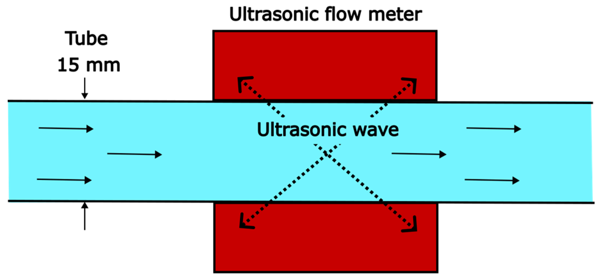
Figure 4.
General overview of the modelling process.

Figure 5.
Schematic diagram of the general MLP structure.

Figure 6.
Schematic diagram of the bagging method applied in EXT.

Figure 7.
Gas holdup in BC1 () and BC2 () and the liquid circulation rate (LCR) () for different superficial gas velocities ().
Figure 7.
Gas holdup in BC1 () and BC2 () and the liquid circulation rate (LCR) () for different superficial gas velocities ().
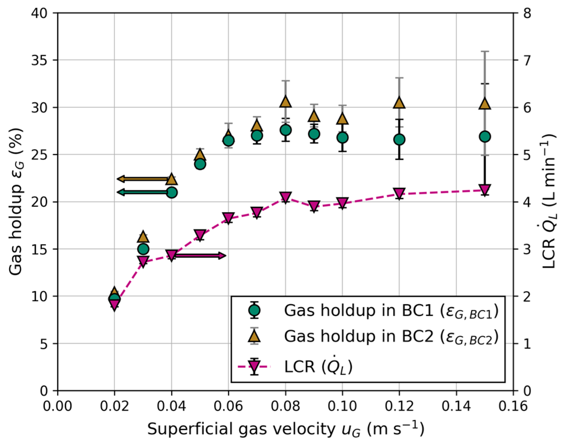
Figure 8.
Influence of superficial gas velocity () on the liquid circulation rate (): (a) effect of different liquid levels (); (b) effect of water quality expressed in different electrical conductivities ().
Figure 8.
Influence of superficial gas velocity () on the liquid circulation rate (): (a) effect of different liquid levels (); (b) effect of water quality expressed in different electrical conductivities ().

Figure 9.
Influence of water quality expressed in different electrical conductivities () on gas holdup () at different superficial gas velocities (): (a) in BC1 and (b) in BC2.
Figure 9.
Influence of water quality expressed in different electrical conductivities () on gas holdup () at different superficial gas velocities (): (a) in BC1 and (b) in BC2.

Figure 10.
Influence of superficial gas velocity () on the liquid circulation rate (): (a) effect of different liquid exit heights (); (b) effect of different tube inner diameters ().
Figure 10.
Influence of superficial gas velocity () on the liquid circulation rate (): (a) effect of different liquid exit heights (); (b) effect of different tube inner diameters ().

Figure 11.
Dependency of the liquid circulation rate () on total gas holdup () and total gas volume flow () for different reactor configurations: Tube inner diameter (), electrical conductivity () and liquid exit height ().
Figure 11.
Dependency of the liquid circulation rate () on total gas holdup () and total gas volume flow () for different reactor configurations: Tube inner diameter (), electrical conductivity () and liquid exit height ().

Figure 12.
The predicted () and experimental () liquid circulation rate for different reactor configurations: tube inner diameter (), electrical conductivity () and liquid exit height (); parity plot of training and testing data for both models: (a) extra trees and (b) multilayer perceptron.
Figure 12.
The predicted () and experimental () liquid circulation rate for different reactor configurations: tube inner diameter (), electrical conductivity () and liquid exit height (); parity plot of training and testing data for both models: (a) extra trees and (b) multilayer perceptron.

Table 3.
Metric results and HP tuning runtime for both models with training and testing data.
| Model | EXT | MLP | ||
|---|---|---|---|---|
| Training | Testing | Training | Testing | |
| MAPE (%) | 1.1 | 4.5 | 3.4 | 5.3 |
| R2 | 0.99 | 0.95 | 0.96 | 0.93 |
| HP tuning (s) | <60 | >9000 | ||
Disclaimer/Publisher’s Note: The statements, opinions and data contained in all publications are solely those of the individual author(s) and contributor(s) and not of MDPI and/or the editor(s). MDPI and/or the editor(s) disclaim responsibility for any injury to people or property resulting from any ideas, methods, instructions or products referred to in the content. |
© 2024 by the authors. Licensee MDPI, Basel, Switzerland. This article is an open access article distributed under the terms and conditions of the Creative Commons Attribution (CC BY) license (https://creativecommons.org/licenses/by/4.0/).
Share and Cite
MDPI and ACS Style
Asbahr, W.; Lamparter, R.; Rauch, R. A Cold Flow Model of Interconnected Slurry Bubble Columns for Sorption-Enhanced Fischer–Tropsch Synthesis. ChemEngineering 2024, 8, 52. https://doi.org/10.3390/chemengineering8030052
AMA Style
Asbahr W, Lamparter R, Rauch R. A Cold Flow Model of Interconnected Slurry Bubble Columns for Sorption-Enhanced Fischer–Tropsch Synthesis. ChemEngineering. 2024; 8(3):52. https://doi.org/10.3390/chemengineering8030052
Chicago/Turabian StyleAsbahr, Wiebke, Robin Lamparter, and Reinhard Rauch. 2024. "A Cold Flow Model of Interconnected Slurry Bubble Columns for Sorption-Enhanced Fischer–Tropsch Synthesis" ChemEngineering 8, no. 3: 52. https://doi.org/10.3390/chemengineering8030052