
Geomorphological Evolution in the Tidal Flat of a Macro-Tidal Muddy Estuary, Hangzhou Bay, China, over the Past 30 Years

 , , , , ,
Abstract
:
1. Introduction
2. Methodology
2.1. Field Data and Remote Sensing Data
2.1.1. Study Area and Field Data
2.1.2. Remote Sensing Data
2.2. Calculation of Tidal Flat Parameters
2.2.1. Elevation
2.2.2. Waterline and Areas
2.2.3. Slope
2.2.4. Vegetation
2.2.5. Tidal Creek
- (1)
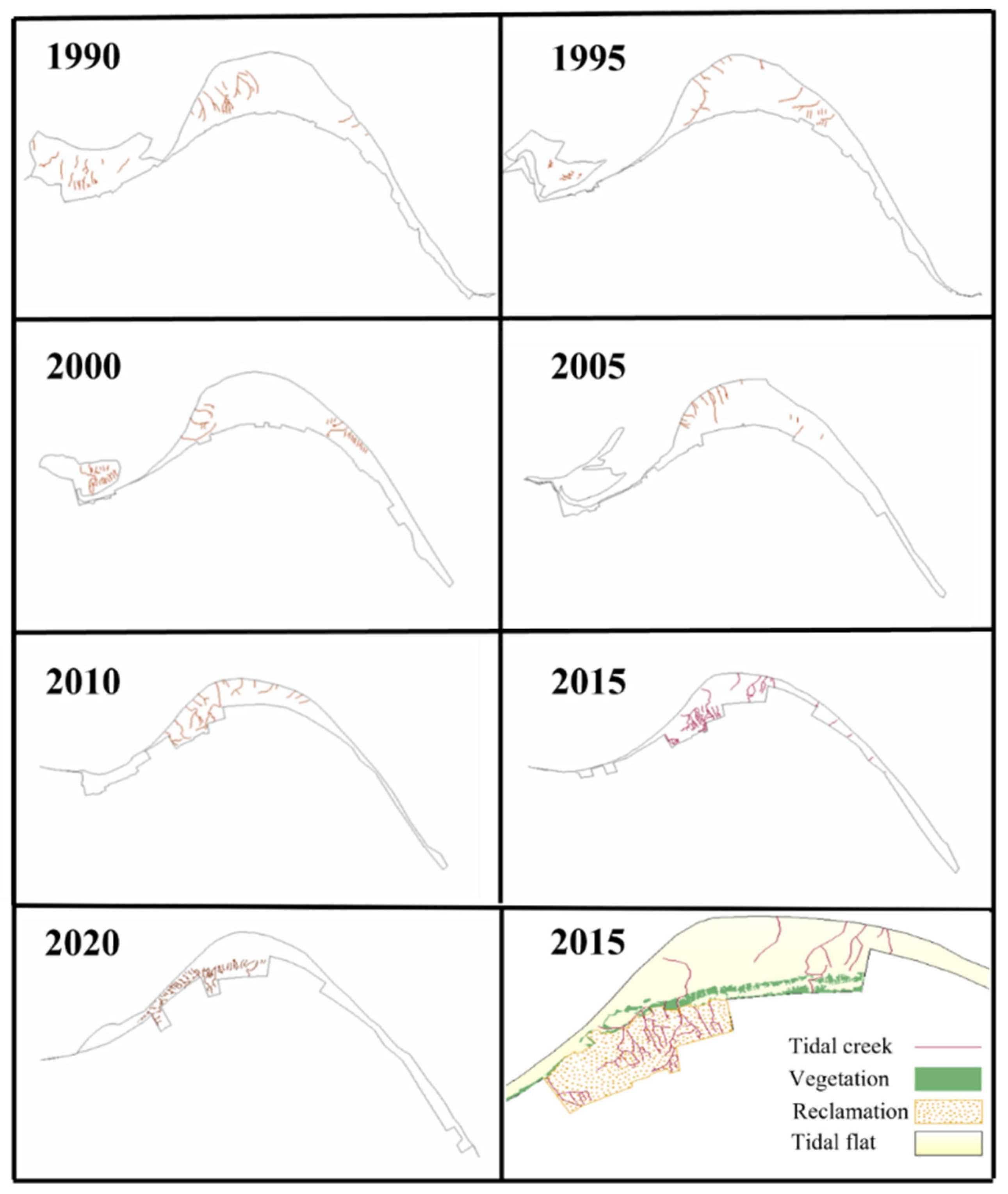
- Tidal creek classification. The Horton–Strahler grading method [64,69] was used to classify tidal creeks. The tidal creek extending directly to the origin of the tidal creek (landward end) was classified as grade 1. There is no bifurcation in the grade 1 tidal trench; two or more grade 1 tidal creeks merge into grade 2, numbered successively until the entire tidal creek system is covered. If two tidal creeks of different grades merge simultaneously, the higher-grade tidal creek is counted (Figure 4d) [70].
- (2)
- Curvature of the tidal creek. The tidal creek curvature was used to represent the curvature of the tidal creek, and its value was equal to the ratio of the total length of the tidal creek to the straight-line distance from the origin of the tidal creek to the point of entry into the sea. The greater the curvature of the tidal creek, the higher the curvature of the tidal creek.
- (3)
- Bifurcation rate of the tidal creek. The bifurcation rate of the tidal creek is an important index used to characterize the development of the tidal creek system, and its value is equal to the number of tidal creek intersection points in one unit of the tidal flat area [24]. The higher the bifurcation rate, the more mature the tidal creek system.
- (4)
- Swing rate of the tidal creek. The tidal creek swing rate was used to quantitatively characterize the stability and spatial variation of the tidal creek system. Its value is the average annual horizontal swing distance of the tidal creek (m/y) [71].
3. Results
3.1. Elevation
3.2. Area
3.3. Slope
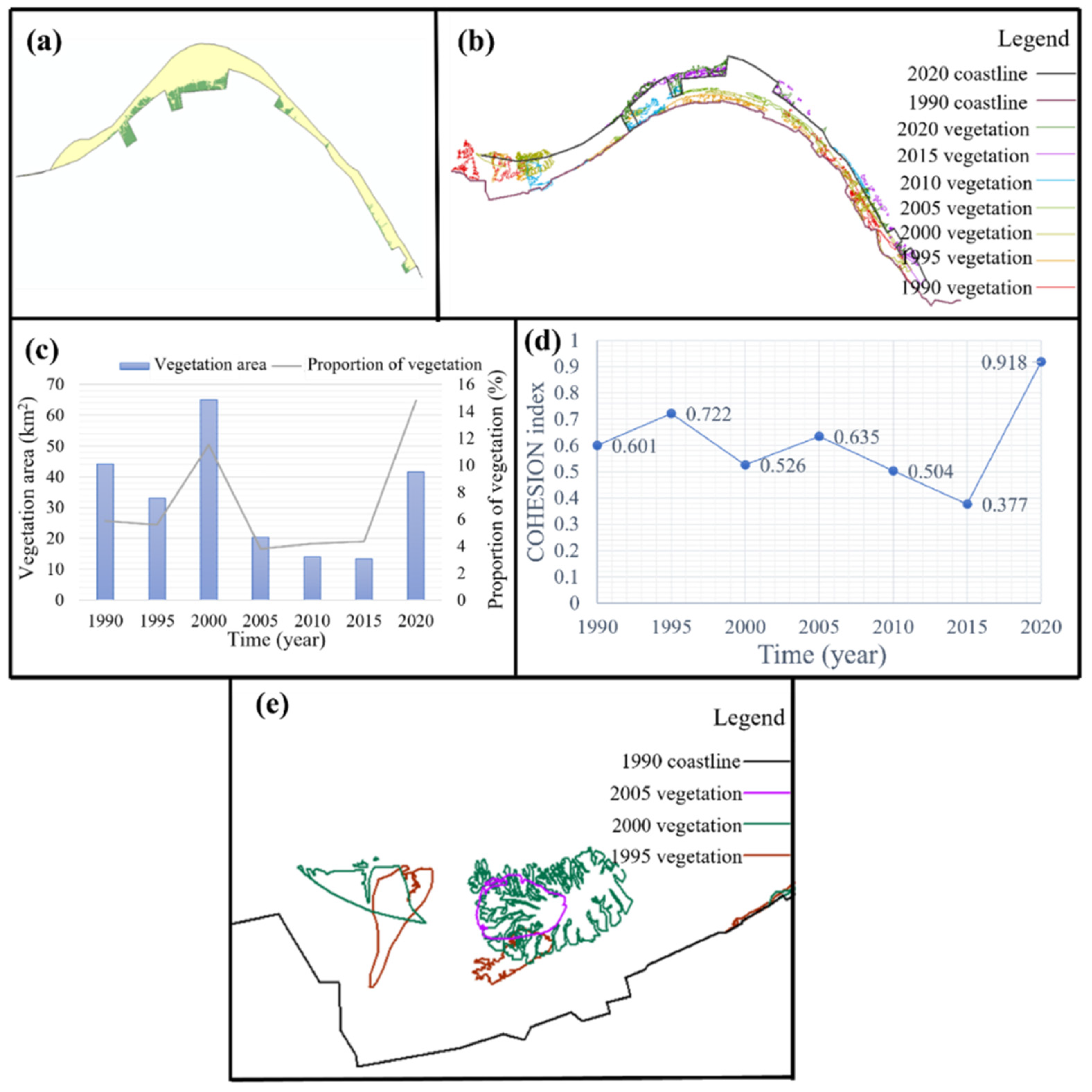
3.4. Vegetation
3.5. Tidal Creeks
4. Discussion
4.1. Impacts of Human Activity on Tidal Flat
4.2. Correlation between Vegetation and Tidal Creek
4.3. Uncertainty Analysis
5. Conclusions
Author Contributions
Funding
Data Availability Statement
Conflicts of Interest
References
- Zhang, C.; Gong, Z.; Chen, Y.; Tao, J.; Kang, Y.; Zhou, J.; Zhou, Z. Research progress and frontier problems of tidal flat evolution. In Proceedings of the 18th China Symposium on Ocean (Shore) Engineering, Zhoushan, China, 23–25 September 2017. [Google Scholar]
- Gong, Z.; Huang, S.; Xu, B.; Zhu, S.; Zhang, Y.; Zhou, Z. Evolution of tidal flat in response to storm surges: A case study from the central Jiangsu Coast. Adv. Water Sci. 2019, 30, 243–254. [Google Scholar]
- Gong, Z.; Zhang, Y.; Zhao, F.; Zhou, Z.; Zhang, C. Advances in coastal storm impacts on morphological evolution of mud tidal flat-creek system. Adv. Sci. Technol. Water Resour. 2019, 39, 75–84. [Google Scholar]
- Hu, C.; Pan, C.; Wu, X.; Tang, Z.; Zheng, J. Tidal flat evolution law and its mechanism on the south bank of Hangzhou Bay from 1959 to 2019. Adv. Water Sci. 2021, 32, 230–241. [Google Scholar]
- Yang, Y.; Wang, Y.; Gao, S.; Wang, X.; Shi, S.; Zhou, L.; Li, G. Sediment resuspension in tidally dominated coastal environments: New insights into the threshold for initial movement. Ocean. Dyn. 2016, 66, 401–417. [Google Scholar] [CrossRef]
- Zhang, X.; Chen, Y.; Le, Y.; Zhang, D.; Yan, Q.; Dong, Y.; Han, W.; Wang, L. Nearshore bathymetry based on ICESat-2 and multispectral images: Comparison between Sentinel-2, Landsat-8, and Testing Gaofen-2. IEEE J. Sel. Top. Appl. Earth Obs. Remote Sens. 2022, 15, 2449–2462. [Google Scholar] [CrossRef]
- Hsu, H.; Haung, C.; Jasinski, M.; Li, Y.; Gao, H.; Yamanokuchi, T.; Wang, C.; Chang, T.; Ren, H.; Kuo, C.; et al. A semi-empirical scheme for bathymetric mapping in shallow water by ICESat-2 and Sentinel-2: A case study in the South China Sea. J. Photogramm. Remote Sens. 2021, 178, 1–19. [Google Scholar] [CrossRef]
- Xu, N.; Ma, Y.; Yang, J.; Wang, X.; Wang, Y.; Xu, R. Deriving tidal flat topography using ICESat-2 laser altimetry and Sentinel-2 imagery. Geophys. Res. Lett. 2022, 49, e2021GL096813. [Google Scholar] [CrossRef]
- Yang, J.; Ma, Y.; Zheng, H.; Xu, N.; Zhu, K.; Wang, X.; Li, S. Derived depths in opaque waters using ICESat-2 photon-counting lidar. Geophys. Res. Lett. 2022, 49, e2021GL100509. [Google Scholar] [CrossRef]
- Zhang, X.; Lin, P.; Gong, Z.; Li, B.; Chen, X. Wave attenuation by Spartina alterniflora under macro-tidal and storm surge conditions. Wetlands 2022, 40, 2151–2162. [Google Scholar] [CrossRef]
- Brodie, J.; Roland, C.; Stehn, S.; Smirnova, E. Variability in the expansion of trees and shrubs in boreal Alaska. Ecology 2019, 100, e02660. [Google Scholar] [CrossRef]
- Marani, M.; Lanzoni, S.; Zandolin, D.; Seminara, G.; Rinaldo, A. Tidal meanders. Water Resour. Res. 2002, 38, 1225. [Google Scholar] [CrossRef]
- Lao, C.; Xin, P.; Zuo, Y.; Cheng, L. Effect of fractional vegetation cover on the evolution of tidal creeks of the Jiuduansha shoal in Yangtze River Estuary (China) during 1996–2020. Adv. Water Sci. 2022, 33, 15–26. [Google Scholar]
- Wu, Y.; Wang, Y.; Zhang, Z. Effects of tidal creek morphology on succession of wetland plant communities in the Yellow River Delta. Ecol. Sci. 2020, 39, 33–41. [Google Scholar]
- Li, J.; Yang, X.; Tong, Y.; Zhang, D.; Shen, Y.; Zhang, R. Influences of Spartina alterniflora invasion on ecosystem services of coastal wetland and its countermeasures. Mar. Sci. Bull. 2005, 24, 33–38+4. [Google Scholar]
- Liu, J.; Yang, S.; Shi, B.; Luo, X.; Fu, X. Topography and evolution of the tidal trench in the eastern Chongming tidal flat, Changjiang River Estuary. J. Mar. Sci. 2012, 30, 43–50. [Google Scholar]
- Chen, Y.; He, Z.; Li, B.; Zhao, B. Spatial distribution of tidal creeks and quantitative analysis of its driving factors in Chongming Dongtan, Shanghai. J. Jilin Univ. (Earth Sci. Ed.) 2013, 43, 212–219. [Google Scholar]
- Liu, L.; Qu, F.; Li, Y.; Yu, J.; Yang, J.; An, C. Correlation between creek tidal distribution and vegetation coverage in the Yellow River Delta coastal wetland. Chin. J. Ecol. 2020, 39, 1830–1837. [Google Scholar] [CrossRef]
- Li, Y.; Wu, H.; Zhang, S.; Lu, X.; Lu, K. Morphological characteristics and changes of tidal creeks in coastal wetlands of the Yellow River Delta under Spartina alterniflora invasion and continuous expansion. Wetl. Sci. 2021, 19, 88–97. [Google Scholar]
- Yu, X.; Han, G.; Wang, X.; Zhang, B. Effects of Spartina alterniflora invasion on morphological characteristics of tidal creeks and plant community distribution in the Yellow River Estuary. Chin. J. Ecol. 2022, 41, 42–49. [Google Scholar] [CrossRef]
- Gong, Z.; Bai, X.; Ji, C.; Zhao, F.; Zhou, Z.; Zhang, C. A numerical model for the cross-shore profile evolution of tidal flats based on vegetation growth and tidal processes. Adv. Water Sci. 2018, 29, 877–886. [Google Scholar]
- Yang, S.; Shi, Z.; Zhao, S. Influence of tidal marsh plants on dynamic sedimentation process in the Yangtze River Estuary. Acta Oceanol. Sin. 2001, 4, 75–80. [Google Scholar]
- Zhou, Z.; Chen, L.; Lin, W.; Luo, F.; Chen, X.; Zhang, C. Advances in bio-geomorphology of tidal flat-saltmarsh systems. Adv. Water Sci. 2021, 32, 470–484. [Google Scholar]
- Mou, K.; Gong, Z.; Qiu, H. Spatiotemporal differentiation and development process of tidal creek network morphological characteristics in Yellow River Delta. Acta Geogr. Sin. 2021, 76, 2312–2328. [Google Scholar] [CrossRef]
- Zhang, C.; Chen, X. Offshore environment changes and countermeasures in response to large-scale tidal flat reclamation. J. Hohai Univ. 2015, 43, 424–430. [Google Scholar]
- Li, J.; Yang, X.; Tong, Y. Progress on environmental effects of tidal flat reclamation. Prog. Geogr. 2007, 26, 43–51. [Google Scholar]
- Chen, L.; Zhou, Z.; Xu, F.; Jiménez, M.; Tao, J.; Zhang, C. Simulating the impacts of land reclamation and de-reclamation on the morphodynamics of tidal networks. Anthr. Coasts 2020, 3, 30–42. [Google Scholar] [CrossRef]
- Lu, B.; Jiang, X. Reclamation impacts on the evolution of the tidal flat at Chongming Eastern Beach in Changjiang estuary. J. Remote Sens. 2013, 17, 342–349+335–341. [Google Scholar]
- Syvitski, J.P.M. Deltas at risk. Sustain. Sci. 2008, 3, 23–32. [Google Scholar] [CrossRef]
- Wei, W.; Dai, Z.; Mei, X.; Gao, S.; Liu, J. Multi-decadal morpho-sedimentary dynamics of the largest Changjiang estuarine marginal shoal: Causes and implications. Land Degrad. Dev. 2019, 30, 2048–2063. [Google Scholar] [CrossRef]
- Dai, Z.; Fagherazzi, S.; Gao, S.; Mei, X.; Ge, Z.; Wei, W. Scaling properties of estuarine beaches. Mar. Geol. 2018, 404, 130–136. [Google Scholar] [CrossRef]
- Yang, G.; Wang, X.; Zhong, Y.; Oliver, T. Modelling study on the sediment dynamics and the formation of the flood-tide delta near Cullendulla Beach in the Batemans Bay, Australia. Mar. Geol. 2022, 452, 106910. [Google Scholar] [CrossRef]
- Guo, L.; Zhu, C.; Xu, F.; Xie, W.; van der Wegen, M.; Townend, I.; Wang, Z.; He, Q. Reclamation of tidal flats within tidal basins alters centennial morphodynamic adaptation to sea-level rise. J. Geophys. Res.-Earth Surf. 2022, 127, e2021JF006556. [Google Scholar] [CrossRef]
- Dai, Z.; Mei, X.; Darby, S.; Lou, Y.; Li, W. Fluvial sediment transfer in the Changjiang (Yangtze) river-estuary depositional system. J. Hydrol. 2018, 566, 719–734. [Google Scholar] [CrossRef]
- Yuan, R.; Zhang, H.; Qiu, C.; Wang, Y.; Guo, X.; Wang, Y.; Chen, S. Mapping morphodynamic variabilities of a meso-tidal flat in Shanghai based on satellite-derived data. Remote Sens. 2022, 14, 4123. [Google Scholar] [CrossRef]
- Zheng, G.; Wang, Y.; Zhao, C.; Dai, W.; Kattel, G.; Zhou, D. Quantitative analysis of tidal creek evolution and vegetation variation in silting muddy flats on the Yellow sea. Remote Sens. 2023, 15, 5107. [Google Scholar] [CrossRef]
- Han, Q. Research on the Status of Tidal Resources in China Using Remote Sensing Technology; Nanjing Normal University: Nanjing, China, 2011. [Google Scholar]
- Ye, T. The Multi-Scale Variations of Suspended Sediment Dynamics in Hangzhou Bay and Its Interaction with Tidal Flat Variations; Zhejiang University: Zhejiang, China, 2019. [Google Scholar]
- Hu, Y.; Yu, Z.; Zhou, B.; Li, Y.; Yin, S.; He, X.; Peng, X.; Shum, C. Tidal-driven variation of suspended sediment in Hangzhou Bay based on GOCI data. Int. J. Appl. Earth Obs. Geoinf. 2019, 82, 101920. [Google Scholar] [CrossRef]
- Liu, Y.; Huang, J.; Xie, D.; Huang, S.; Ying, C.; Li, L. Impact of SSC distribution in Hangzhou Bay after 1307 typhoon through satellite images. Hydro-Sci. Eng. 2021, 6, 9–16. [Google Scholar]
- Huang, J.; Yuan, R.; Zhu, J. Numerical Simulation and Analysis of Water and Suspended Sediment Transport in Hangzhou Bay, China. J. Mar. Sci. Eng. 2022, 10, 1248. [Google Scholar] [CrossRef]
- Zhu, L.; Huang, Y.; Yang, G.; Sun, W.; Chen, C.; Huang, K. Information extraction and spatio-temporal evolution analysis of the coastline in Hangzhou Bay based on Google Earth Engine and remote sensing technology. Remote Sens. Nat. Resour. 2023, 35, 50–60. [Google Scholar]
- Wang, S.; Xu, M.; Han, Y.; Gao, G.; Huang, H. Analysis and scenario prediction of multi-year blue carbon in intertidal wetland on the south bank of Hangzhou Bay. China Environ. Sci. 2022, 42, 4380–4388. [Google Scholar]
- Fang, Q.; Huang, S.; Xu, X.; Wang, J.; Li, D.; Xie, H. Analysis of the influence of reclamation engineering group on the accumulated hydrodynamics in the south coast of Hangzhou Bay. Sci. Technol. Eng. 2020, 20, 5338–5344. [Google Scholar]
- Li, L.; Ren, Y.; Ye, T.; Wang, X.H.; Huang, J.; Xia, Y. Positive feedback between the tidal flat variations and sediment dynamics: An example study in the macro-tidal turbid Hangzhou Bay. J. Geophys. Res.-Ocean. 2023, 128, e2022JC019414. [Google Scholar] [CrossRef]
- Tian, Q.; Zheng, L.; Tong, Q. Atmospheric radiation correction and reflectance inversion method based on remote sensing imagery. J. Appl. Meteorol. Sci. 1998, 77–82. [Google Scholar]
- Gens, G. Remote sensing of coastlines: Detection, extraction and monitoring. Int. J. Remote Sens. 2010, 31, 1819–1836. [Google Scholar] [CrossRef]
- Awange, J.; Saleem, A.; Sukhadiya, R.; Ouma, Y.; Kexiang, H. Physical dynamics of Lake Victoria over the past 34 years (1984–2018): Is the lake dying? Sci. Total Environ. 2019, 658, 199–218. [Google Scholar] [CrossRef] [PubMed]
- Amos, C.L. Chapter 10 Siliciclastic Tidal Flats. Dev. Sedimentol. 1995, 53, 273–306. [Google Scholar]
- Zhang, Y.; Gao, Z.; Liu, X.; Xu, N. The extraction method of tidal flat area based on remote sensing waterlines. Ocean Dev. Manag. 2018, 35, 56–61. [Google Scholar]
- Han, Z.; Guo, Y. Waterside line information extraction of tidal flat at the Yangtze River Estuary by wavelet multi-resolution analysis. Mar. Sci. 2011, 35, 67–70. [Google Scholar]
- Li, X.; Zhang, H. Edge detection algorithm of gray image. Electron. Opt. Control 2018, 25, 46–49. [Google Scholar]
- Dong, Z.; Fu, D.; Liu, D.; Yu, G.; Zhang, X. Study on the extraction of waterline with different landforms based on ZY-3 remote sensing images. Hydrogr. Surv. Charting 2019, 39, 34–39. [Google Scholar]
- Luo, M.; Zhang, D. Research on accurate extraction of waterline under conditions of blurred water-land boundary. Mar. Sci. 2019, 43, 106–112. [Google Scholar]
- Bi, J.; Zhang, L.; Wang, P.; Sui, Y.; Mu, X.; Wang, P. Improved mathematical morphology-based image segmentation algorithm for coastline extraction and its region adaptability analysis. Geogr. Geo-Inf. Sci. 2019, 35, 20–29. [Google Scholar]
- Yan, H.; Li, B.; Chen, M. Progress of researches in coastline extraction based on RS technique. Areal Res. Dev. 2009, 28, 101–105. [Google Scholar]
- Egbert, G.D.; Erofeeva, S.Y. Efficient Inverse Modeling of Barotropic Ocean Tides. J. Atmos. Ocean. Technol. 2002, 19, 183–204. [Google Scholar] [CrossRef]
- Hua, Y. Study on the Expansion of Reclamation and Land Use Changes in Hangzhou Bay; Zhejiang University: Zhejiang, China, 2016. [Google Scholar]
- Zhang, X.; Zhang, X.; Yang, B.; Zhuang, Z.; Shang, K. Coastline extraction using remote sensing based on coastal type and tidal correction. Remote Sens. Land Resour. 2013, 25, 91–97. [Google Scholar]
- Chen, W.; Zhang, D.; Cui, D.; Lv, L.; Xie, W.; Shi, S.; Hou, Z. Monitoring spatial and temporal changes in the continental coastline and the intertidal zone in Jiangsu province, China. Acta Geogr. Sin. 2018, 73, 1365–1380. [Google Scholar]
- Sha, H.; Zhang, D.; Cui, D.; Lv, L.; Ni, P. Remote sensing prediction method of coastline based on self-adaptive profile morphology. Acta Oceanol. Sin. 2019, 41, 170–180. [Google Scholar]
- Liu, Y.; Cong, P.; Li, J.; Wei, B.; Dai, J.; Han, C. A morphological analysis of tidal creek in the Yellow River Delta based on remote sensing. Mar. Environ. Sci. 2020, 39, 393–398. [Google Scholar]
- Huete, A.; Didan, K.; Marani, M.; Rodriguez, E.P.; Gao, X.; Ferreira, L.G. Overview of the radiometric and biophysical performance of the MODIS vegetation indices. Remote Sens. Environ. 2002, 83, 195–213. [Google Scholar] [CrossRef]
- Arthur, S. Dynamic basis of geomorphology. Geol. Soc. Am. Bull. 1952, 63, 923–938. [Google Scholar]
- Meng, M.; Tian, H.; Wu, M.; Wang, L.; Niu, Z. Analysis of the Evolution of Wetland Landscape Spatial Pattern Based on Google Earth Engine Platform: Taking Baiyangdian as an Example. J. Yunnan Univ. Nat. Sci. Ed. 2019, 41, 416–424. [Google Scholar]
- Lin, S. Study on Water Information Extraction Method of GF-1 Image Based on the Combination of NDVI and Modified FCM; Geomatics & Spatial Information Technology: Harbin, China, 2017. [Google Scholar]
- Dubey, Y.; Mushrif, M.; Mitra, K. Brain tumor detection and segmentation using multiscale intuitionistic fuzzy roughness in MR images. Biomed. Eng. -Appl. Basis Commun. 2019, 31, 1950020. [Google Scholar] [CrossRef]
- Chen, H.; Chen, C.; Zhang, Z.; Wang, L.; Liang, J. A remote sensing information extraction method for intertidal zones based on Google Earth Engine. Remote Sens. Nat. Resour. 2022, 34, 60–67. [Google Scholar]
- Horton, R.E. Erosional development of streams and their drainage basins: Hydrophysical approach to quantitative morphology. Bull. Geol. Soc. Am. 1945, 56, 275–370. [Google Scholar] [CrossRef]
- Hao, X. Study on the Morphological Characteristics and Evolution of Tidal Trenches on the Land Shore of Jiangsu Radiation Sandbar; Nanjing Normal University: Nanjing, China, 2021. [Google Scholar]
- Liu, Y.; Li, J.; Zhang, Y.; Zhao, X.; Xu, W.; He, G.; Liu, Y. Dynamic monitoring of vegetation in Southern Hangzhou Bay from time series images. J. Ningbo Univ. (Nat. Sci. Eng. Ed.) 2020, 30, 25–31. [Google Scholar]
- Pettorelli, N.; Vik, J.O.; Mysterud, A.; Gaillard, J.; Tucker, C.; Stenseth, N. Using the satellite-derived NDVI to assess ecological responses to environmental change. Trends Ecol. Evol. 2005, 20, 503–510. [Google Scholar] [CrossRef] [PubMed]
- Carol, A.; Wilson, Z.; FitzGerald, D.; Hopkinson, C.; Valentine, V.; Kolker, A. Saltmarsh pool and tidal creek morphodynamics: Dynamic equilibrium of northern latitude saltmarshes? Geomorphology 2014, 213, 99–115. [Google Scholar]
- Kearney, W.S.; Fagherazzi, S. Salt marsh vegetation promotes efficient tidal channel networks. Nat. Commun. 2016, 7, 12287. [Google Scholar] [CrossRef]
- Ye, M.; Li, J.; Shi, X.; Jiang, Y.; Shi, Z.; Xu, L.; He, G.; Huang, R.; Feng, B. Spatial pattern change of the coastline development and utilization in Zhejiang from 1990 to 2015. Geogr. Res. 2017, 36, 1159–1170. [Google Scholar]
- Ren, Y. Characteristics and Mechanism of Suspended Sediment in Hangzhou Bay Considering Wave-Current Interaction; Zhejiang University: Zhejiang, China, 2022. [Google Scholar]
- Zheng, X.; Zhou, B.; Lei, H.; Huang, Q.; Ye, H. Extraction and spatio-temporal change analysis of the tidal flat in Cixi section of Hangzhou Bay based on Google earth engine. Remote Sens. Nat. Resour. 2022, 34, 18–26. [Google Scholar]
- Jafari, R.; Sui, J. Velocity Field and Turbulence Structure around Spur Dikes with Different Angles of Orientation under Ice Covered Flow Conditions. Water 2021, 13, 1844. [Google Scholar] [CrossRef]
- Dai, Z.; Liu, J. Impacts of large dams on downstream fluvial sediment: An example of the Three Gorges Dam (TGD) on the Changjiang (Yangtze River). J. Hydrol. 2013, 480, 10–18. [Google Scholar] [CrossRef]
- Dai, Z.; Liu, J.; Wei, W.; Chen, J. Detection of the Three Gorges Dam influence on the Changjiang (Yangtze River) submerged delta. Sci. Rep. 2014, 4, 6600. [Google Scholar] [CrossRef] [PubMed]
- Xie, D.; Pan, C.; Cao, Y.; Zhang, B. Decadal variations in the erosion/deposition pattern of the Hangzhou Bay and their mechanism in recent 50a. Haiyang Xuebao 2013, 35, 121–128+9. [Google Scholar]
- Fu, Y.; Yin, P.; Gao, F.; Liu, D.; Cao, K.; Tian, Y. Remote sensing study on Spartina alterniflora in the northern tidal flat of Sanmen Bay in Zhejiang Province. Period. Ocean Univ. China 2002, 52, 134–144. [Google Scholar]
- Lou, Y.; Dai, Z.; Long, C.; Dong, H.; Wei, W.; Ge, Z. Image-based machine learning for monitoring the dynamics of the largest salt marsh in the Yangtze River Delta. J. Hydrol. 2022, 608, 127681. [Google Scholar] [CrossRef]


| Data Identifier | Date * | Flood/Dry | Cloud Cover (%) | Notes |
|---|---|---|---|---|
| LT51180391990162HAJ00 | 11 June 1990 | Flood | 0.13 | Near high-water level |
| LT51180391990226HAJ00 | 14 August 1990 | Flood | — | |
| LT51180391990338HAJ00 | 4 December 1990 | Dry | — | Near low-water level |
| LT51180391995192HAJ00 | 11 July 1995 | Flood | 0.22 | Near high-water level |
| LT51180391995224HAJ00 | 12 August 1995 | Flood | — | |
| LT51180391995256CLT02 | 13 September 1995 | Flood | 14.27 | Near low-water level |
| LT51180391999043HAJ00 | 12 February 1999 | Dry | 1.37 | Near low-water level |
| LT51180391999091HAJ00 | 1 April 1999 | Normal | 0.46 | |
| LT51180392000158HAJ03 | 6 June 2000 | Flood | 6.12 | Near high-water level |
| LT51180392004201BJC00 | 19 July 2004 | Flood | 14.22 | Near high-water level |
| LT51180392005155BJC00 | 4 June 2005 | Flood | 0.56 | |
| LT51180392005331BJC00 | 27 November 2005 | Dry | — | Near low-water level |
| LT51180392009198BJC00 | 17 July 2009 | Flood | 0.07 | Near high-water level |
| LT51180392010313BJC00 | 9 November 2010 | Dry | — | |
| LT51180392010361BJC00 | 27 December 2010 | Dry | 5.00 | Near low-water level |
| LC81180392015023LGN00 | 23 January 2015 | Dry | 18.80 | Near low-water level |
| LC81180392015071LGN00 | 12 March 2015 | Normal | 2.74 | |
| LC81180392015215LGN00 | 3 August 2015 | Flood | 0.50 | Near high-water level |
| LC81180392020133LGN00 | 12 May 2020 | Flood | 18.01 | Near high-water level |
| LC81180392020229LGN00 | 16 August 2020 | Flood | 9.23 | |
| LC81180392021087LGN00 | 28 March 2021 | Normal | 15.73 | Near low-water level |
| Section | 8# | 14# | 19# | 24# | 28# | 36# | Date |
|---|---|---|---|---|---|---|---|
| Tidal level (m) | −0.77 | −0.03 | 0.62 | 0.78 | 0.52 | 0.27 | 28 March 2021 (Low water level) |
| −0.22 | −0.23 | −0.19 | −0.13 | −0.12 | −0.11 | 16 August 2020 (Medium water level) | |
| −1.12 | −0.55 | 0.15 | 0.11 | 0.11 | 0.17 | 12 May 2020 (High water level) | |
| Horizontal projection distance (km) | 0.34 | 0.16 | 2.05 | 0 | 1.19 | 0 | 28 March 2021 (Low water level) |
| 0.84 | 1.81 | 3.11 | 0.01 | 1.46 | 0.87 | 16 August 2020 (Medium water level) | |
| 1.72 | 2.83 | 8.68 | 2.11 | 2.72 | 1.53 | 12 May 2020 (High water level) | |
| Average slope | 0.24 | 0.2 | 0.1 | 0.43 | 0.703 | 0.07 |
| Section | 8# | 14# | 19# | 24# | 28# | 36# | Time (Year) |
|---|---|---|---|---|---|---|---|
| Average slope | −1.07 | 0.33 | 1.48 | 0.99 | 0.79 | −0.78 | 1990 |
| 1.71 | 0.32 | 0.238 | 0.16 | 0.589 | 2.61 | 1995 | |
| 1.47 | 0.29 | 0.24 | 0.27 | 0.25 | 0.05 | 2000 | |
| −1.45 | 0.327 | 0.25 | 0.27 | 0.95 | −0.02 | 2005 | |
| 1.21 | 0.527 | 0.36 | 0.58 | 0.95 | 2.07 | 2010 | |
| −1.53 | 0.27 | 0.42 | 0.20 | 0.89 | 0.36 | 2015 | |
| 0.24 | 0.2 | 0.1 | 0.43 | 0.7 | 0.07 | 2020 |
| Year | Number | The Ratios of Each Grade (%) | Parameters | ||||||
|---|---|---|---|---|---|---|---|---|---|
| Grade 1 | Grade 2 | Grade 3 | Grade 4 | Length (km) | Density (km/km2) | Curvature | Branching Rate (per km2) | ||
| 1990 | 51 | 0.75 | 0.2 | 0.06 | 0 | 112.54 | 0.15 | 1.01 | 0.03 |
| 1995 | 41 | 0.83 | 0.17 | 0 | 0 | 73.89 | 0.13 | 1.03 | 0.03 |
| 2000 | 64 | 0.84 | 0.14 | 0 | 0 | 96.19 | 0.17 | 1.070 | 0.04 |
| 2005 | 21 | 0.86 | 0.14 | 0 | 0 | 45.95 | 0.09 | 1.04 | 0.01 |
| 2010 | 26 | 0.85 | 0.15 | 0 | 0 | 81.46 | 0.24 | 1.15 | 0.03 |
| 2015 | 77 | 0.70 | 0.2 | 0.08 | 0.03 | 105.93 | 0.34 | 1.07 | 0.19 |
| 2020 | 117 | 0.74 | 0.18 | 0.06 | 0.03 | 105.83 | 0.38 | 1.11 | 0.24 |
Disclaimer/Publisher’s Note: The statements, opinions and data contained in all publications are solely those of the individual author(s) and contributor(s) and not of MDPI and/or the editor(s). MDPI and/or the editor(s) disclaim responsibility for any injury to people or property resulting from any ideas, methods, instructions or products referred to in the content. |
© 2024 by the authors. Licensee MDPI, Basel, Switzerland. This article is an open access article distributed under the terms and conditions of the Creative Commons Attribution (CC BY) license (https://creativecommons.org/licenses/by/4.0/).
Share and Cite
Li, L.; Shen, F.; Xia, Y.; Shi, H.; Wang, N.; He, Z.; Gao, K. Geomorphological Evolution in the Tidal Flat of a Macro-Tidal Muddy Estuary, Hangzhou Bay, China, over the Past 30 Years. Remote Sens. 2024, 16, 1702. https://doi.org/10.3390/rs16101702
Li L, Shen F, Xia Y, Shi H, Wang N, He Z, Gao K. Geomorphological Evolution in the Tidal Flat of a Macro-Tidal Muddy Estuary, Hangzhou Bay, China, over the Past 30 Years. Remote Sensing. 2024; 16(10):1702. https://doi.org/10.3390/rs16101702
Chicago/Turabian StyleLi, Li, Fangzhou Shen, Yuezhang Xia, Haijing Shi, Nan Wang, Zhiguo He, and Kai Gao. 2024. "Geomorphological Evolution in the Tidal Flat of a Macro-Tidal Muddy Estuary, Hangzhou Bay, China, over the Past 30 Years" Remote Sensing 16, no. 10: 1702. https://doi.org/10.3390/rs16101702