Article

Classification of Pollution Sources and Their Contributions to Surface Water Quality Using APCS-MLR and PMF Model in a Drinking Water Source Area in Southeastern China

1
College of Water Conservancy Engineering, Tianjin Agricultural University, Tianjin 300392, China
2
State Key Laboratory of Hydrology and Water Resources and Hydraulic Engineering Science, Nanjing Hydraulic Research Institute, Nanjing 210029, China
3
State Key Laboratory of Hydroscience and Engineering, Department of Hydraulic Engineering, Tsinghua University, Beijing 100084, China
*
Author to whom correspondence should be addressed.
Water 2024, 16(10), 1356; https://doi.org/10.3390/w16101356
Submission received: 29 March 2024 / Revised: 16 April 2024 / Accepted: 22 April 2024 / Published: 10 May 2024
(This article belongs to the Section Urban Water Management)

Abstract

:
Identifying the potential pollution sources of surface water pollutants is essential for the management and protection of regional water environments in drinking water source areas. In this study, absolute principal component score-multiple linear regression (APCS-MLR) and positive matrix factorization (PMF) models were applied to assess water quality and identify the potential pollution sources affecting the surface water quality of Xin’an River Basin. For this purpose, a 10-year (2011–2020) dataset of eight water quality indicators (including pH, EC, DO, COD, NH3-N, TN, TP, and FC) covering eight monitoring stations and 7248 monthly observations was used. The results indicated that Pukou section had the worst water quality among the eight monitoring stations, and TN was the most serious water quality index. Both the APCS-MLR and PMF models identified agricultural nonpoint source pollution, urban nonpoint source pollution and rural domestic pollution, and meteorological factors. The sum of these three sources was very close, accounting for 60% and 58%, respectively. The APCS-MLR results demonstrated that for EC, COD, and NH3-N, the major pollution sources were urban nonpoint sources and rural domestic pollution. The major contamination source of TN was agricultural nonpoint source pollution (30.4%). Meanwhile, the major pollution sources of pH, DO, TP, and FC were unidentified factors. The PMF model identified five potential sources, and pH and DO were affected by meteorological factors. NH3-N and TP were influenced mainly by agricultural nonpoint source pollution. Atmospheric deposition was the major pollution source (87.9%) of TN. FC was mostly derived from livestock and poultry breeding (88.3%). EC and COD were mostly affected by urban nonpoint sources and rural domestic pollution. Therefore, receptor models can help managers identify the major sources of pollution in watersheds, but the major factors affecting different pollutants need to be supplemented by other methods.

1. Introduction

Water quality problems pose serious threats to human health, ecology, and the environment and have attracted widespread attention worldwide [1,2]. Moreover, with the development of technology, water quality monitoring has become easier; it mainly relies on sampling analysis and automated monitoring stations [3]. Meanwhile, extensive water quality parameters are available, and many watersheds have accumulated a large amount of observed data [4]. Thus, the question of how to effectively use these data to help the government formulate corresponding policies to control water quality is a critical issue.
The surface water quality is affected by multiple factors, including natural factors and several anthropogenic factors [5]. The natural factors include catchment lithology, topography, and climate and atmospheric deposition [6]. The anthropogenic factors include domestic sewage, industrial wastewater, agricultural activities, and livestock breeding. Rivers have been under great pressure [7] because of increasing concentrations of nutrients, organics, heavy metals, and other pollutants [8,9]. These pollutants are discharged in the form of point sources or nonpoint sources. Nonpoint source pollution, which is mainly a season-dependent phenomenon influenced by rainfall runoff processes, carries various pollutants from urban areas and agricultural fields [10]. Compared with point source pollutants, nonpoint source pollutants have greater spatial and temporal variabilities and are relatively easy to deposit and degrade within a river network [11]. Therefore, it is important to find an easy way to analyze potential pollution sources and identify the relationships between various pollutants and their sources.
Pollution source analysis methods can be divided into two categories: forward traceability and reverse traceability [12]. Forward traceability begins from the process of pollutants entering a river and is calculated mostly by the pollution source inventory method and the watershed model method. The traditional pollution source inventory method relies mainly on the use of a top-down approach to calculate the discharge of each pollution source or the amount of water into the river (lake). However, determining the export coefficient of pollutants is difficult, and the spatiotemporal heterogeneity of the pollution source discharge coefficient is very large [13]. Watershed models such as the SWAT [14], HSPF [15], and AGNPS [16] models are principally based on mathematical methods used to reproduce the physical process of pollutant migration in a basin. However, these models are complex, require a large amount of input data and long-term practice, and are difficult to apply in the analysis of regional pollution sources lacking data. Reverse traceability mainly starts with river water quality data and reveals the sources of different pollutants through certain methods, including isotope analysis and receptor modeling. Isotope analysis can be traced only to specific pollutants; for example, nitrogen isotopes can be traced only to nitrogen. As another important element affecting water eutrophication, phosphorus cannot be traced to phosphorus isotopes, as only one stable isotope of phosphorus exists in nature [17]. Thus, the receptor model is a better choice for source analysis in areas with a large amount of observed data.
The absolute principal component score-multiple linear regression (APCS-MLR) model, which was proposed by Thurston and Spengler [18], combines principal component analysis (PCA) and MLR. This model was applied to confirm the contribution of each possible source defined by PCA [19]. Combined with multiple linear regression, the contributions of major pollution factors to the water quality of the recipient were quantified [20]. It was initially applied to the analysis of air pollution sources and has been widely applied to the analysis of soil [21,22], groundwater [23], and surface water pollution sources [24] in recent years [25]. However, the PCA model, which identifies the type of pollution source, revealed a certain degree of subjectivity [8]. The positive matrix factorization (PMF) model is a new source analysis model improved on the basis of factor analysis that can apply nonnegative constraints to the factorization matrix to increase the accuracy of the results. It is a source analysis tool recommended by the US EPA [26,27]. The APCS-MLR and PMF models are the most commonly used methods for the quantitative apportionment of the contribution of pollution sources [28,29]. Previous studies have combined APCS-MLR and PMF to identify the source apportionment of soil heavy metals [30,31]. A few studies have focused on storm runoff pollution [32], groundwater pollution [23], and surface water quality [29].
Due to the global shortage of water resources and the deterioration of water quality, drinking water safety, water source protection, and other related issues were widely considered worldwide in the second half of the 20th century [33,34]. The Xin’anjiang Reservoir is an important source of drinking water for the Yangtze River Delta region of China and provides drinking water for more than 20 million people [35]. Previous studies have shown that since the pilot of the basin ecological compensation mechanism, the water quality of the Xin’an River has improved on the whole, but there was also local water pollution and unstable water quality in transit sections. With the acceleration of upstream industrialization and urbanization, various pollutants are more likely to increase, and the water quality of some reaches of the Xin’an River showed a downward trend. In particular, the total nitrogen (TN) and total phosphorus (TP) in some sections exceeded the standard [36,37]. Many studies have focused on nonpoint source pollution upstream of the Xin’anjiang Reservoir [35,38,39]; however, few studies have conducted overall traceability analyses of regional pollutant sources. On the other hand, drinking water source basins have higher water quality requirements, lower concentrations of pollutants, and fewer pollution sources than other areas. All these methods are similar to heavy metal and groundwater pollution traceability methods. Thus, in this paper, the upper reaches of the Xin’an River Basin (XRB) were used to analyze the water quality and pollutant sources from 2011 to 2020 via the APCS-MLR and PMF models. The major objectives include the following: (1) to identify the spatio-temporal characteristics of the water quality; (2) to classify the major sources of surface water pollution and quantitatively analyze the contributions of different pollution sources to each water quality index; and (3) to compare the two receptor models to provide a more reliable method for analyzing similar catchments. The results of this study may be helpful for the method selection of pollution source apportionment and surface water environment management in similar basins.

2. Materials and Methods

2.1. Study Area and Data

2.1.1. Study Area

The XRB is located between 29°29′~30°14′ N and 117°38′~118°54′ E in southeastern China, with a total area of 5760 km2. The average annual temperature is between 15 °C and 16 °C, and the average annual precipitation is approximately 1700 mm [35]. However, the spatial and temporal distributions are uneven, and most of the precipitation is concentrated in the flood season from May to August. The vegetation types in the study area are diverse, with forest coverage accounting for approximately 75% of the total area and agricultural land accounting for approximately 15%. The specific distribution is shown in Figure 1. The XRB is the main water source for Qiandao Lake and an important ecological safety barrier in the Yangtze River Delta. For many years, the overall water quality upstream of Xin’an River has been stable, and the water quality has remained at Class II–III (the class of water quality was assessed according to the National Surface Water Quality Standard of China (GB3838-2002) [40]) annually; the Xin’an River is one of the rivers with less pollution and better water quality in China. In 2011, the state established the first cross-provincial pilot ecological compensation mechanism in the XRB to protect the water environment and control water pollution.

2.1.2. Data Description

Monthly data for 24 water quality indices at 8 monitoring sites along the rivers from 2011 to 2020 were obtained from the Huangshan Municipal Ecology and Environment Bureau. The 25 water quality indices included pH, dissolved oxygen (DO), potassium permanganate index (COD), chemical oxygen demand (CODCr), biochemical oxygen demand (BOD5), ammonia nitrogen (NH3-N), TN, TP, Cu, Zn, fluoride (F), electrical conductivity (EC), fecal coliform (FC), As, Cd, Se, Hg, Cr VI, Pb, cyanide, volatile phenol, petroleum, sulfide, and anionic surfactant (AS). The observed data indicated that 14 indicators (AS, sulfide, petroleum pollution, volatile phenol, Zn, Hg, Pb, Cd, Cr VI, Cu, F, Se, As, and cyanide) were not detected, and 2 indicators (BOD5 and CODcr) were inconsistent. Thus, the other 8 water quality indices were used in this paper. The 8 monitoring sites included Huangkou, Huangdun, Kengkou, Jiekou, Pukou, Xinguan, Shuaishui, and Hengjiang (see Figure 1). The annual point source pollution data from 2011 to 2020, including pollutant concentration and sewage discharge at each sewage outlet, were also provided by the Huangshan Municipal Ecology and Environment Bureau.

2.2. Methodology

2.2.1. Principal Component Analysis (PCA)

PCA is a technique from statistics that is used to simplify a dataset. It was developed by Pearson [41] and Hotelling [42]. The basic principle of PCA is that in the data point graph under the coordinate system, the direction of maximum “fluctuation” of the data point is considered the new axis direction, and the coordinates of the data point on the axis are the first principal component (PC1). The first principal component (PC1) accounts for most of the variation in the original dataset [43]. Then, the second direction, which is perpendicular to the new coordinate and can best reflect the “fluctuation” of the data point, is sought; this direction is taken as the second new coordinate axis direction, and the coordinates of the data points on this axis are the second principal component (PC2); then, all the principal components that can express the original information can be obtained. The application of the PCA method to an evaluation of the water environment quality involves two major steps: (1) to establish a comprehensive evaluation index, the relative pollution degree of each monitoring section is evaluated, and the pollution degree of each monitoring section is ranked; and (2) to evaluate the role of each single index in the comprehensive index, those minor indices are clearly deleted, and the major components causing pollution are determined. Based on field measurements, Olsen et al. [44] demonstrated the advantages of PCA over other methods for better identification of effective pollutant factors across river reaches. In this research, PCA was used to determine the major components causing pollution in the XRB. More details of PCA can be found in other studies [45,46,47,48,49].

2.2.2. Absolute Principal Component Analysis

The APCS-MLR is a receptor model that combines two statistical methods, APCS and MLR. First, the principal components of the water quality index were extracted as the basis for pollution source identification and quantification. The principal component score can be calculated as follows:
P C S j k = i = 1 ω i j Z i k
Z i k = c i k c ¯ i σ i
where P C S j k is the score of principal component j for sample k, ω i j is the factor coefficient of pollutant i for principal component j, Z i k is the standardized value of pollutant i for sample k, and c i k is the observed value of pollutant i for sample k, mg/L. c ¯ i is the arithmetic mean value of pollutant i. σ i is the standard deviation of pollutant i.
The absolute principal component score can be expressed as follows:
A P C S j k = P C S j k P C S j k 0
P C S j k 0 = i = 1 ω i j Z i k 0
Z i k 0 = 0 c ¯ i σ i
where A P C S j k is the score of the absolute component principal j for sample k, and P C S j k 0 is the score of principal component j after the water quality index of sample k is set to 0. Z i k 0 is the standardized value of pollutant i after the water quality index of sample k is set to 0.

2.2.3. Multivariate Linear Regression

Multiple linear regression analysis was carried out to obtain the regression equation. The details can be seen as follows:
C i = j a j i · A P C S j i + b i
where C i is the concentration of pollutant i. a j i indicates the regression coefficient of source j to pollutant i. b i is the constant term of multiple linear regression for pollutant i, which is considered to represent the contributions of unidentified sources. a j i · A P C S j i represents the contribution of pollution source j to C i .
In the past, the calculation results of the contribution rate were positive and negative, which led to contributions of various factors greater than 100%, possibly affecting the accuracy of the pollution source analysis. Gholizadeh et al. [28] proposed the absolute value method to solve this problem, which can be calculated as follows:
P C j i = a j i · A P C S j i ¯ b i + j = 1 n a j i · A P C S j i ¯ × 100 %
The contribution rate of the unidentified source is expressed as follows:
P C j i = b i b i + j = 1 n a j i · A P C S j i ¯ × 100 %
where P C j i is the contribution rate of pollution source j to pollutant i. A P C S j i ¯ is the mean value of the absolute principal factor scores of all samples of pollutant i.

2.2.4. Positive Matrix Factorization (PMF)

The PMF model is a multivariate factor analysis tool. Based on the least iterative square algorithm, the original receptor data matrix (X) is decomposed into a factor score matrix (G), factor load matrix (F), and residual matrix (E) [50]. The formula is as follows:
X i j = k = 1 p G i k × F k j + E i j
where X i j is the observed value of pollutant j for sample i; G i k is the relative contribution rate of pollution source k in sample i; F k j is the characteristic value of pollution source k to pollutant j; E i j is the residual; and p is the number of factors.
The original matrix X is decomposed by the PMF model to obtain the optimal matrices G and F, and the objective function Q is minimized [51]. The objective function Q is defined as follows:
Q = i = 1 n j = 1 m ( E i j U i j ) 2
The operation of the PMF model does not require accurate pollution source data; rather, it requires only original measured data and uncertainty data [52]. The uncertainty U i j is calculated as follows:
U i j = 5 6 × M D L   X i j M D L U i j = ( σ × X i j ) 2 + M D L 2   X i j > M D L
where σ is the relative standard deviation, and MDL is the detection limit of the method.
For PMF source analysis, the factor number is a key factor in the operation of the PMF model. Too much or too little of a factor directly affects the accuracy of the analysis result. The sectional water quality concentration data and uncertainty data were input into the PMF model, and 2–5 factors were set in this study. The program was run several times to compare the output Q value, residual, and R2 of different factors, and the appropriate factor number was ultimately selected.

3. Results

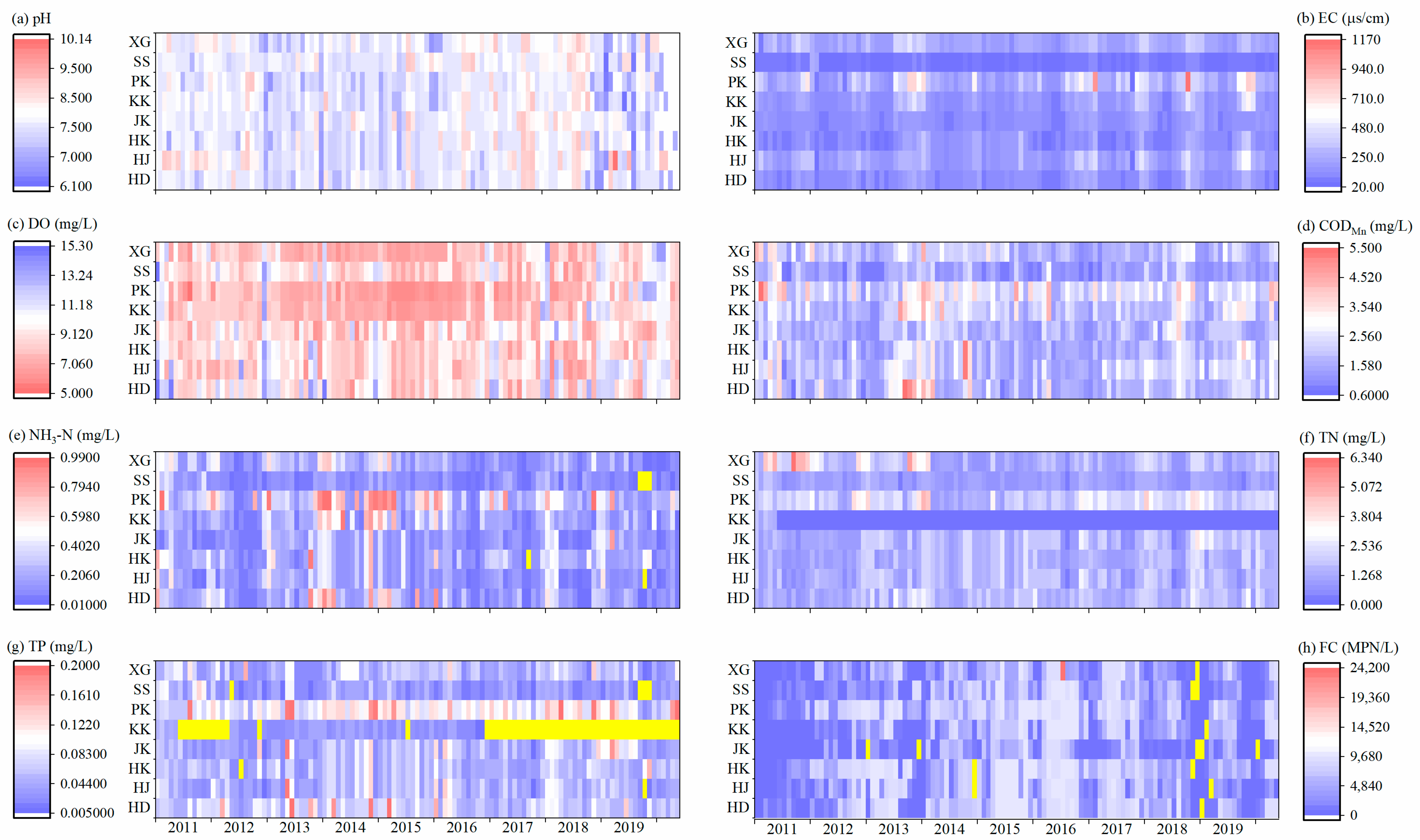
3.1. Variations in Water Quality Indicators
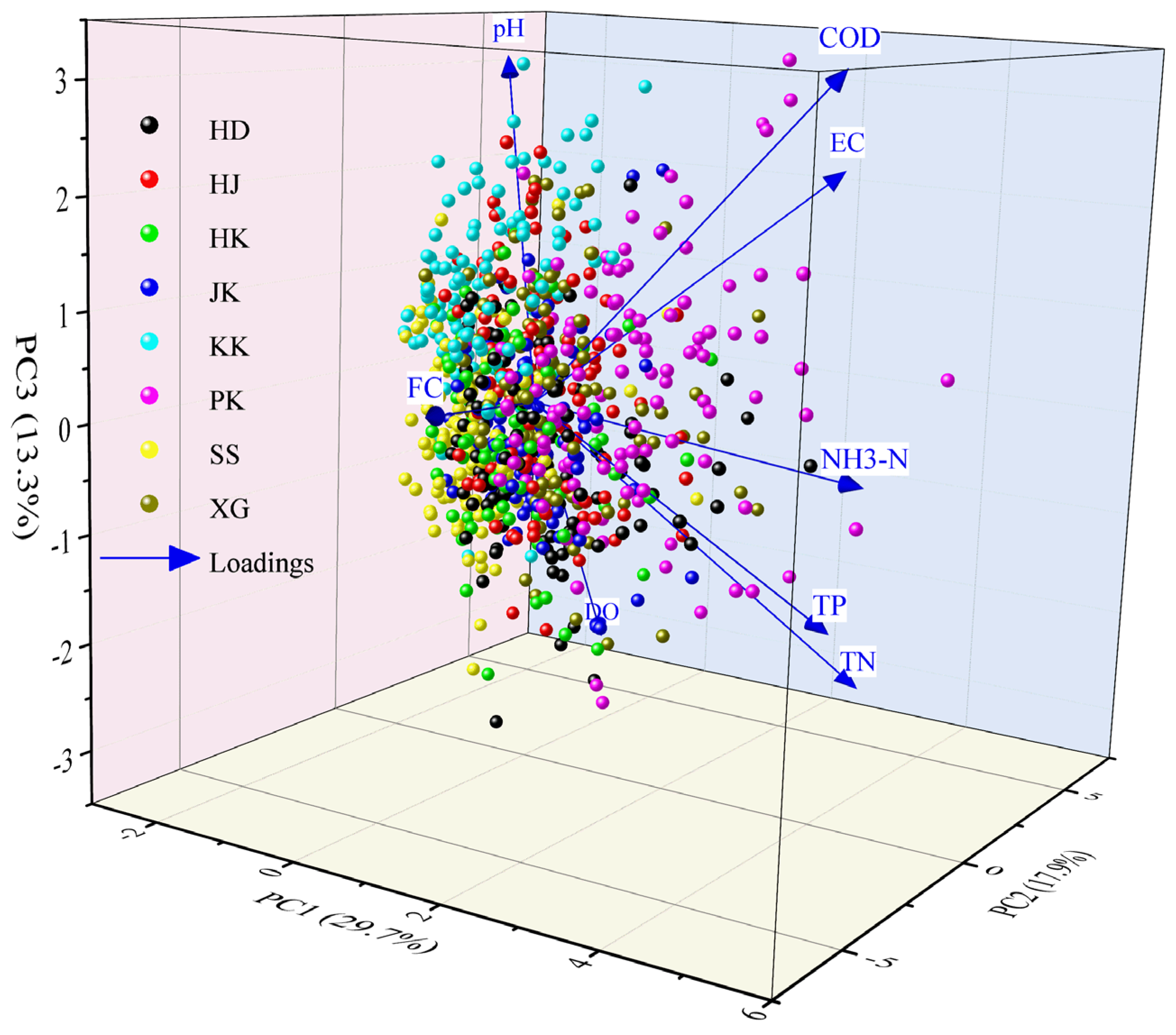
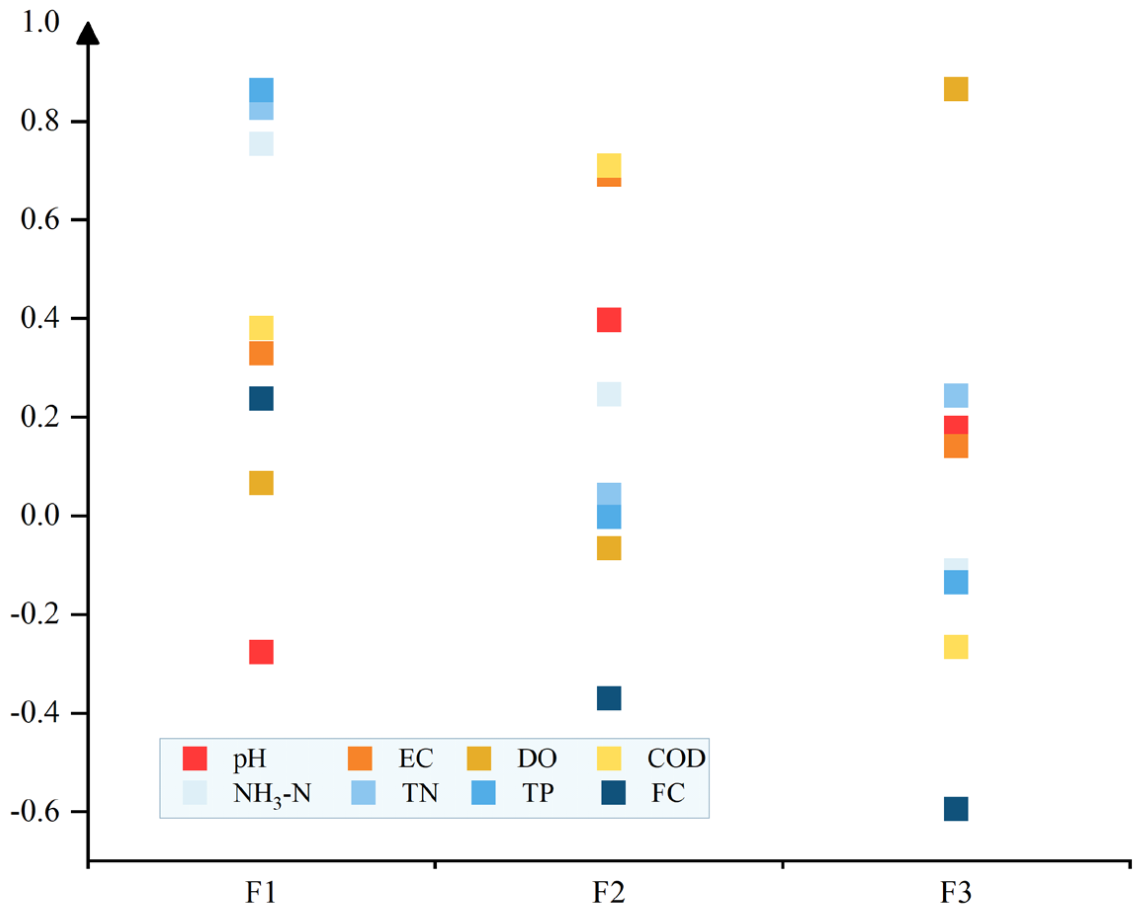
The eight water quality values are presented as the means and standard deviations of the monthly replicates in Table 1. The maximum values of EC, COD, NH3-N, TN, and TP occurred in Pukou. Except for TN, the average values of all the other indicators were above Class II. The average concentrations of TN were more than 1.5 mg/L in addition to Kengkou (0.08 mg/L), Shuaishui (0.99 mg/L), and Huangkou (1.45 mg/L), which exceeded Class IV in the surface water environment. The mean concentration of TN in the Pukou section exceeded the surface water Class V standard.
Figure 2 shows the variations in the monthly water quality indicators from 2011 to 2020 in the different sections. Notably, there was no significant difference in pH across sections. Most of the pH values were between 7 and 8.5 (Figure 2a). Figure 2b illustrates that the EC of Pukou had an abnormally high value in some months, and the values in the other cross sections were generally less than 48. The EC of the SS was low throughout the observation period. The lower DO concentrations were mostly concentrated in Pukou and Kengkou, but most of the observed values were greater than 7 (Figure 2c). According to Figure 2d, the highest COD was 5.5 mg/L (better than that of Class III). Except for Kengkou, the variation characteristics of daily NH3-N and TN were consistent (Figure 2e,f), which indicated that Pukou had the highest mean TN concentration, followed by Xinguan and Huangdun. Moreover, the TN concentration in Xinguan before 2013 was also relatively higher than that in the other years. Jiekou, Huangkou, and Hengjiang had nearly the same values of NH3-N and TN during 2014–2015, as did the TP concentration (Figure 2g). The TN and TP contents in Kengkou were lower than those in the other sections, and TP has not been detected since 2017. From 2015–2016, FC had a higher concentration (less than 10,000) than that in the other periods in all sections, and the highest value of 24,200 MPN/L occurred once in Xinguan in 2016 (Figure 2h).
The variations in the average monthly and annual Nemerow indices of the eight monitoring sections are shown in Figure 3. It can be noted that, whether monthly or annually, the Nemerow index of Pukou was the largest. As seen from the annual index variation, most sections had no significant change trends, except for a significant decrease in Xinguan. Even the basin outlet of Jiekou substantially increased in 2019. The Nemerow index for most sections had its lowest value in September or October (Figure 3a), indicating that the water quality in the study area was the best during these years. Moreover, the highest values of most sectional indices occurred in February and December. This indicated that the water quality in the flood season was better than that in the nonflood season. Rainfall runoff processes are known to carry slope contaminants into rivers, and the discharge also increases. When fewer pollutants were carried into rivers, the pollutant concentration decreased. In the nonflood season, the pollutant concentration may be influenced by point source pollution. Thus, average annual point source pollutant discharge was calculated according to sewage volume and pollutant concentration, and the distributions of point source pollution and the average concentrations of the four indicators are shown in Figure 4. There was no obvious correlation between the spatial distribution of point sources and the water quality of the section. Point pollution may have an influence, but these effects were not significant. For example, statistical results showed that the annual point source TN was nearly 320 t, whereas the nonpoint source TN was more than 18,500 t [35]. NH3-N, TN, and TP may have the same pollution sources, as indicated by the high concentration sections located downstream of farmland. However, for CODCr, the downstream area of construction land, such as Hengjiang, had a high concentration, which may be influenced by urban nonpoint sources.

3.2. PCA Results

The correlation analysis results among the different water quality indices are shown in Figure 5. Previous studies have shown that correlation analysis can reflect correlations and can be used to infer sources. There was a strong positive correlation at the 0.05 significance level between EC and COD, between COD and NH3-N, between NH3-N and TP, and between TN and TP, indicating that these water quality indicators may have similar pollution sources. NH3-N and TN, EC and TN, and COD and TP had moderately significant positive correlations and may have had similar sources. The correlation coefficient between TN and NH3-N was only 0.34, illustrating that NH3-N accounted for only a small part of the TN in the study area. Figure 5 shows that pH and FC were only weakly positively correlated or significantly negatively correlated with other water quality indicators before, which indicated that the sources of these two indicators were significantly different from those of the other indicators.
The original water quality data were standardized, and the Kaiser–Meyer–Olkin (KMO) test and Bartlett’s test results demonstrated that the PCA was valid.
The PCA of eight water quality indices from 2011 to 2020 was calculated with SPSS Statistics 21. The total variance in the principal component interpretation in the XRB is shown in Table 2. According to Kaiser [53], the principle of eigenvalues greater than 1 was selected as the principal component. Thus, three principal components were obtained in the study area, accounting for 60.91% of the total variance in the water quality dataset. Figure 6 shows the 3D coordinates of the principal component axes based on the monitored water quality indices and stations. The sample points of different sections exhibited a certain degree of aggregation, which indicated that the sample points of each section were different but that there were similarities. To reduce the overlap of the original variables, the factor load matrix was orthogonally rotated to determine the main load of the principal component (Figure 7).

3.3. Source Identification

For the APCS-MLP model, a previous study [54] showed that absolute factor loadings of >0.75, [0.5, 0.75], and [0.3, 0.5] were considered strong, moderate, and weak loadings, respectively. Thus, Table 2 and Figure 7 show that in this research, the eigenvalue of the first principal component (F1) was 2.377, the variance contribution rate was 29.719%, and the major load variables included TP, TN, and NH3-N. According to Wang et al. [35], TN and TP loaded during the flood season (April to July) accounted for 65.0% and 63.2%, respectively, of the annual total. Taken together, these results indicated that TN and TP were influenced by rainfall and runoff processes; that is, they mainly originated from nonpoint source pollution. Thus, F1 can be identified as agricultural nonpoint source pollution. The second principal component (F2) eigenvalue was 1.429, the variance contribution rate was 17.858%, and the major load variables included EC and COD. Previous research [38] demonstrated that the spatial distribution of COD was consistent with that of construction land and rural residential land in this region. Therefore, F2 can be identified as an urban nonpoint source and rural domestic pollution. DO was the main load variable of the third principal component (F3), and the eigenvalue and variance contribution rate were 1.067 and 13.334%, respectively. Consequently, F3 was defined as a meteorological factor.
For the PMF model, three to five factors were selected for 20 random starting point iterative operations, and the factor number was 5. The QRobust and QTrue values were the closest (QTrue is the calculated goodness-of-fit parameter, and QRobust is the calculated goodness-of-fit parameter excluding the model that does not fit points). The residuals of all the samples were between −3 and 3, which indicated that the analytical results of the model had good reliability. According to the PMF model, the contribution rate of each pollution source to the water quality indicators was calculated, and the results are shown in Figure 8. Notably, Factor 1 (Figure 8a) in the PMF model had the largest contamination source for FC, with a contribution rate of 88.32%. FCs are a group of intestinal bacteria that grow in the intestines of humans and warm-blooded animals and are excreted in the feces. The toilets of rural residents in the study area have been reformed and are generally not exposed to the outside; thus, Factor 1 can be identified as a source of livestock and poultry breeding pollution. Factor 2 (Figure 8b) had the highest contribution to EC and COD, which were 62.87% and 38.50%, respectively, and was the same as the F2 contribution to APCS-MLR. Thus, Factor 2 can be considered an urban nonpoint source and rural domestic pollution. Factor 3 (Figure 8c) had the highest contribution rate of TN, which was 87.92%. According to Wang et al. [36], the TN load from atmospheric deposition accounts for 65–71% of the total load. Therefore, Factor 3 can be defined as the atmospheric deposition. Factor 4 (Figure 8d) had the highest contribution to pH and DO, which were 58.28% and 65.62%, respectively. These variables were mainly affected by meteorological conditions under natural conditions; thus, Factor 4 can be identified as a meteorological factor. Factor 5 (Figure 8e) had the highest contribution rates to NH3-N and TP, which were 84.23% and 55.27%, respectively. NH3-N and TP were the major pollutants of nonpoint source pollution; thus, Factor 5 can be defined as an agricultural nonpoint source pollution factor.

3.4. Source Pollutant Contributions

A total of 7248 samples and eight pollutants were adopted to qualify the sources that affected the water quality indices, which indicated that the PCA results were reliable in this research [18]. The APCS-MLR model was used to determine the functional relationship between each pollution source and the concentration of water quality indicators. Based on the functional relationship, the concentration of each indicator was predicted, and a linear comparison between the simulated and observed results is shown in Figure 9. According to Figure 9, the R2 of the linear fit between the simulated and observed concentrations of each water quality index in the study area ranged from 0.41 to 0.69, indicating good consistency between the two. In addition, the ratios of the simulated and observed concentrations were close to 1, illustrating that the APCS-MLR model has good applicability for the calculation and allocation of pollution sources in the XRB and that the calculation results are relatively reliable.
Based on the APCS-MLR model and the pollution source contribution model, the contribution rate of each pollution source to the water quality indicator was obtained (Figure 10a). The results demonstrated that for EC, COD, and NH3-N, the major pollution sources were urban nonpoint sources and rural domestic pollution, accounting for 50.4%, 66.2%, and 55.7%, respectively. The main contamination source of TN was agricultural nonpoint source pollution (30.4%), followed by urban nonpoint source and rural domestic pollution (26.0%) and meteorological factors (23.1%). The effects of these factors on TN did not significantly differ, which indicated that TN was affected by comprehensive factors from all aspects. The major pollution sources of the remaining four indicators, pH, DO, TP, and FC, were unidentified factors and represented 73.9%, 54.1%, 46.5%, and 89.1%, respectively, of the total pollution. In addition, the secondary pollution source of DO was meteorological factors (40.0%), and TP was also affected by nonpoint source pollution (26.6%).
Same as the APCS data, the simulation of each water quality index by PMF is shown in Figure 10. All the R2 values were above 0.5, and the slopes were also near 1. The results indicated that the PMF model had good applicability for simulating the surface water quality index, and the traceability analysis of the water quality index based on these results was reliable. The contribution rates of the various pollution sources determined by the PMF model are shown in Figure 11b. Notably, meteorological factors were the major sources of pH and DO. NH3-N and TP were influenced mainly by agricultural nonpoint source pollution, and the contribution rates were 84.2% and 55.3%, respectively. Atmospheric deposition was the main pollution source of TN, accounting for 87.9% of the total. FC was mostly derived from livestock and poultry breeding and accounted for 88.3% of the total population. EC and COD were mostly affected by urban nonpoint sources and rural domestic pollution, accounting for 62.9% and 38.5%, respectively.

3.5. Comparison of the Results

There were some differences between the PMF model and the APCS-MLR model. First, there were no undefined sources of pollution in the PMF model, which made up a significant proportion of the APCS-MLR model, especially for pH, DO, and FC. Unidentified pollution sources accounted for 73.9%, 54.1%, and 89.1% of the total contribution rates of pH, DO, and FC, respectively. Second, the contribution rates of the same pollution source to different pollutants also differed from those of the APCS-MLR model. Taking NH3-N as an example, both methods revealed that NH3-N was affected by agricultural nonpoint source pollution, urban nonpoint sources and rural domestic pollution, and meteorological factors. However, the contribution rates of the three factors were 27.7%, 55.6%, and 8.8%, respectively, in the APCS-MLR model. According to the PMF model, the contribution rates of the three factors were 84.2%, 14.0%, and 1.7%, respectively. Moreover, the identification results of influencing factors for the same pollutant were also different. For example, in the APCS-MLR model, TN was affected by a variety of factors, and the contribution rates of the different factors were not significantly different. However, in the PMF model, TN was mainly affected by atmospheric deposition, with a contribution rate of 87.9%.
To evaluate the applicability of the APCS-MLR and PMF models for the analysis of surface water quality pollution sources, the ratios of the observed and simulated surface water quality concentrations (O/S) and the coefficient of determination (R2) were further analyzed (Table 3). According to Shi et al. [55], when O/S is close to 1 and R2 is greater than 0.5, the source allocation results are considered reliable. The results showed that the simulated values of the two models fit well with the observed values. Except for the pH of APCS-MLR, the R2 values of the other water quality indicators were greater than 0.5, indicating that the reliability of the source analysis results was high. As shown in Table 3, the O/S value of APCS-MLR was basically 1, but the R2 value of the PMF model was generally greater than that of APCS-MLR. A comparison of Figure 9 and Figure 10 reveals that the distribution of points in the PMF model was more concentrated than that in the APCS-MLR model, but most of the water quality indicators were underestimated.
The average contribution rates of the various pollution sources determined with the APCS-MLR and PMF models are shown in Figure 12. The results indicated that both models identified agricultural nonpoint source pollution, urban nonpoint source pollution and rural domestic pollution, and meteorological factors. The sum of these three sources was very close, accounting for 60% and 58%, respectively. In APCS-MLR, the proportions of the three pollution sources were 15%, 29%, and 16%, respectively. In the PMF model, the proportions of the three pollution sources were 21%, 16%, and 21%, respectively. This was mainly because the basic principles of the two models were different. The APCS-MLR model yielded a few independent factors (pollution sources) that could explain the main information in the dataset by means of dimensionality reduction, after which the contribution rate of each pollution source was calculated via linear regression. The PMF model evaluated the error of each point in the dataset to determine the optimal number of pollution sources and the corresponding contribution rate. The remaining 40% of the APCS-MLR data were unidentified, which was also a major shortcoming of the model. According to the PMF model, the remaining 42% were associated with atmospheric deposition (27%) and livestock and poultry breeding pollution (15%). In general, the PMF model is more accurate in this basin, and the analytical results of the two models complement and verify each other and provide theoretical support for later management departments to formulate surface water quality source control measures.

4. Discussion

Nitrogen is one of the main causes of lake eutrophication. Only NH3-N, and not TN (measured by the lake), is considered in surface water quality standards. As seen from the previous analysis, the concentration of NH3-N in the river was better than that in Class II, but the TN concentration in most sections reached only Class IV in this region. However, the study area was the main inflow river of Qiandao Lake, accounting for 60.2% of the total runoff [56]. Thus, the TN of rivers is likely to greatly impact TN of lakes, and understanding the source river TN is important for controlling and protecting the water environment of Qiandao Lake. The APCS-MLR results indicated that TN was affected by comprehensive factors, including agricultural nonpoint source pollution (30.4%), urban nonpoint source and rural domestic pollution (26.0%), and meteorological factors (23.1%), in the study area. There was no significant difference in the degree of influence of the different factors on the TN. However, the results of the PMF model indicated that TN was influenced mainly by atmospheric deposition and accounted for 87.9% of the total TN. According to Wang et al. [35], the TN load from atmospheric deposition accounts for 65–71% of the total. On the other hand, about 75% of the study area is forest, and 15% is farmland. In 2011, the state established the first cross-provincial pilot ecological compensation mechanism in the XRB to protect the water environment and control water pollution. Meanwhile, the study area is surrounded by major cities such as Nanjing, Shanghai, and Hangzhou (see Figure 1). Thus, it is reasonable to believe that agricultural non-point source pollution was not the main source of TN in the study area; rather, it was atmospheric nitrogen deposition. However, to effectively control the TN concentration in the study area, multiple simultaneous approaches are needed. On the other hand, in current source analysis methods based on statistical methods, identifying pollution sources involves a certain subjectivity, which is one of the important sources of uncertainty in source analysis calculations. Thus, more detailed research should be carried out based on the compositional characteristics of the source in the future, and other methods should be used to further analyze the source of TN in the study area to test the reliability of the results.

5. Conclusions

In this study, eight pollutants were collected from 7248 samples during 2011 to 2020 in the XRB, and the APCS-MLR and PMF models were used to identify pollutant sources. Due to differences in model principles, the quantitative identification of pollution sources was also different, but there were still some similarities. According to the results, the following conclusions can be drawn:
(1)
The observed water quality analysis results showed that the water quality of Pukou was the worst among the eight monitored sections, and the maximum values of EC, COD, NH3-N, TN, and TP occurred in Pukou. In addition to TN, the average values of the other water quality indicators were above Class II. The variation characteristics of daily NH3-N and TN were consistent. The Nemerow index was the largest for Pukou. Most sections had no significant annual change trends, except for a significant decrease in Xinguan.
(2)
The results of the correlation analysis demonstrated that EC and COD, COD and NH3-N, NH3-N and TP, and TN and TP may have similar pollution sources. The sources of pH and FC were significantly different from other indicators.
(3)
For APCS-MLR, three pollution sources were defined. For EC, COD, and NH3-N, the major pollution sources were urban nonpoint sources and rural domestic pollution, accounting for 50.4%, 66.2%, and 55.7%, respectively. The major contamination source of TN was agricultural nonpoint source pollution (30.4%). The major pollution sources of pH, DO, TP, and FC were unidentified factors, which represented 73.9%, 54.1%, 46.5%, and 89.1%, respectively, of the total pollution.
(4)
For the PMF model, five pollution sources were defined. pH and DO were affected by meteorological factors. NH3-N and TP were influenced mainly by agricultural nonpoint source pollution, and the contribution rates were 84.2% and 55.3%, respectively. Atmospheric deposition was the main pollution source (87.9%) of TN. FC was mostly derived from livestock and poultry breeding (88.3%). EC and COD were mostly affected by urban nonpoint sources and rural domestic pollution, accounting for 62.9% and 38.5%, respectively.
(5)
Both models identified agricultural nonpoint source pollution, urban nonpoint source pollution and rural domestic pollution, and meteorological factors. The sum of these three sources was very close, accounting for 60% and 58%, respectively. The remaining 40% of the APCS-MLRs were unidentified. According to the PMF model, the remaining 42% were associated with atmospheric deposition (27%) and livestock and poultry breeding pollution (15%).

Author Contributions

Methodology, A.W.; software, J.W.; validation, B.L.; formal analysis, A.W.; investigation, Z.W.; resources, S.W.; data curation, S.W.; writing—original draft preparation, A.W.; writing—review and editing, D.Y.; visualization, A.W.; supervision, S.W.; project administration, A.W.; funding acquisition, A.W. All authors have read and agreed to the published version of the manuscript.

Funding

This research was funded by the National Natural Science Foundation of China, “Simulation of nonpoint source pollution and identification in the water source basin” (Project No. 52109062); and the Project of the Scientific Research Program of the Tianjin Municipal Education Commission (Grant No. 2017KJ189).

Data Availability Statement

Data are contained within the article.

Conflicts of Interest

The authors declare no conflicts of interest.

References

  1. Brown, T.C.; Froemke, P. Nationwide assessment of nonpoint source threats to water quality. BioScience 2012, 62, 136–146. [Google Scholar] [CrossRef]
  2. Saksena, D.; Garg, R.; Rao, R. Water quality and pollution status of Chambal river in National Chambal sanctuary, Madhya Pradesh. J. Environ. Biol. 2008, 29, 701–710. [Google Scholar] [PubMed]
  3. Ren, X.; Cheng, Y.; Zhao, B.; Xiao, J.; Gao, D.; Zhang, H. Water quality assessment and pollution source apportionment using multivariate statistical and PMF receptor modeling techniques in a sub-watershed of the upper Yangtze River, Southwest China. Environ. Geochem. Health 2023, 45, 6869–6887. [Google Scholar] [CrossRef] [PubMed]
  4. Mester, T.; Benkhard, B.; Vasvári, M.; Csorba, P.; Kiss, E.; Balla, D.; Fazekas, I.; Csépes, E.; Barkat, A.; Szabó, G. Hydrochemical Assessment of the Kisköre Reservoir (Lake Tisza) and the Impacts of Water Quality on Tourism Development. Water 2023, 15, 1514. [Google Scholar] [CrossRef]
  5. Iqbal, J.; Shah, M.H. Occurrence, risk assessment, and source apportionment of heavy metals in surface sediments from khanpur lake, pakistan. J. Anal. Sci. Technol. 2014, 5, 28. [Google Scholar] [CrossRef]
  6. Summya, N.; Zeshan, A.; Riffat, N. Water quality assessment of river Soan (Pakistan) and source apportionment of pollution sources through receptor modelling. Arch. Environ. Contam. Toxicol. 2016, 71, 97–112. [Google Scholar]
  7. Koundouri, P. Current issues in the economics of groundwater resource management. J. Econ. Surv. 2010, 18, 703–740. [Google Scholar] [CrossRef]
  8. Cheng, G.; Wang, M.; Chen, Y.; Gao, W. Source apportionment of water pollutants in the upstream of Yangtze River using APCS-MLR. Environ. Geochem. Health 2020, 42, 3795–3810. [Google Scholar] [CrossRef]
  9. Moya, C.E.; Raiber, M.; Taulis, M.; Cox, M.E. Hydrochemical evolution and groundwater flow processes in the Galilee and Eromanga basins, Great Artesian Basin, Australia: A multivariate statistical approach. Sci. Total Environ. 2015, 508, 411–426. [Google Scholar] [CrossRef]
  10. Singh, K.P.; Malik, A.; Mohan, D.; Sinha, S. Multivariate statistical techniques for the evaluation of spatial and temporal variations in water quality of Gomti River (India)—A case study. Water. Res. 2004, 38, 3980–3992. [Google Scholar] [CrossRef]
  11. Wang, A.; Tang, L.; Yang, D. Spatial and temporal variability of nitrogen load from catchment and retention along a river network: A case study in the upper Xin’anjiang catchment of China. Hydrol. Res. 2016, 47, 869–887. [Google Scholar] [CrossRef]
  12. Hou, X.K.; Zhang, K.; Duan, P.Z.; Wang, X.; Ta, L.; Guo, Y.; Xia, R. Pollution source apportionment of Tuohe River Based on absolute principal component score-multiple linear regression. Res. Environ. Sci. 2021, 34, 2350–2357. [Google Scholar]
  13. Hou, X.K.; Zhan, X.Y.; Zhou, F.; Yan, X.Y.; Gu, B.J.; Reis, S.F.; Wu, Y.L.; Liu, H.B.; Piao, S.L.; Tang, Y.H. Detection and attribution of nitrogen runoff trend in China’s croplands. Environ. Pollut. 2018, 234, 270–278. [Google Scholar] [CrossRef]
  14. Arnold, J.G.; Allen, P.M.; Bernhardt, G. A comprehensive surface-groundwater flow model. J. Hydrol. 1993, 142, 47–69. [Google Scholar] [CrossRef]
  15. Bicknell, B.R.; Imhoff, J.C.; Kittle, J.L. Hydrological Simulation Program: Fortran; User’s manual for release 10; U.S. Environmental Protection Agency: Washington, DC, USA, 1993.
  16. Young, R.A.; Onstad, C.A.; Bosch, D.D.; Anderson, W.P. AGNPS: A nonpoint-source pollution model for evaluating agricultural watersheds. J. Soil. Water. Conserv. 1989, 44, 168–173. [Google Scholar]
  17. Ji, J.; Xu, Z. Progress on tracing sources and biogeochemical cycling of phosphorus by using oxygen isotopes of phosphate. Environ. Sci. Technol. 2010, 33, 360–363. [Google Scholar]
  18. Thurston, G.D.; Spengler, J.D. A quantitative assessment of source contributions to inhalable particulate matter pollution in metropolitan Boston. Atmos. Environ. 1985, 19, 9–25. [Google Scholar] [CrossRef]
  19. Zhou, F.; Liu, Y.; Guo, H. Application of multivariate statistical methods to water quality assessment of the watercourses in Northwestern New Territories, Hong Kong. Environ. Monit. Assess. 2007, 132, 1–13. [Google Scholar] [CrossRef] [PubMed]
  20. Shi, W.; Gu, Z.; Feng, Y. Source apportionment of heavy metals in sediments with application of APCS-MLR model in Baoxiang River. Environ. Sci. Technol. 2020, 43, 51–59. [Google Scholar]
  21. Guan, Q.; Zhao, R.; Pan, N.; Wang, F.; Yang, Y.; Luo, H. Source apportionment of heavy metals in farmland soil of Wuwei, China: Comparison of three receptor models. J. Clean. Prod. 2019, 237, 117792.1–117792.10. [Google Scholar] [CrossRef]
  22. Wu, J.; Margenot, A.J.; Wei, X.; Fan, M.; Zhang, H.; Best, J.L.; Wu, P.; Chen, F.; Gao, C. Source apportionment of soil heavy metals in fluvial islands, Anhui section of the lower Yangtze River: Comparison of APCS–MLR and PMF. J. Soil. Sediment. 2020, 20, 3380–3393. [Google Scholar] [CrossRef]
  23. Zhang, H.; Cheng, S.; Li, H.; Fu, K.; Xu, Y. Groundwater pollution source identification and apportionment using PMF and PCA-APCA-MLR receptor models in a typical mixed land-use area in Southwestern China. Sci. Total Environ. 2020, 741, 140383. [Google Scholar] [CrossRef] [PubMed]
  24. Liu, L.; Tang, Z.; Kong, M.; Chen, X.; Zhou, C.; Huang, K.; Wang, Z. Tracing the potential pollution sources of the coastal water in Hong Kong with statistical models combining APCS-MLR. J. Environ. Manag. 2019, 245, 143–150. [Google Scholar] [CrossRef] [PubMed]
  25. Liu, Z.; Ding, C.; Chao, J.; Zheng, Z.; Cui, Y. Pollution source apportionment of Changtan Reservoir of Zhejiang province based on APCS-MLR model. J. Ecol. Rural Environ. 2023, 39, 530–539. [Google Scholar]
  26. Wang, S.; Cai, L.M.; Wen, H.H.; Luo, J.; Wang, Q.S.; Liu, X. Spatial distribution and source apportionment of heavy metals in soil from a typical county-level city of Guangdong province, China. Sci. Total Environ. 2019, 655, 92–101. [Google Scholar] [CrossRef]
  27. Wang, Y.; Li, Y.; Yang, S.; Liu, J.; Zheng, W.; Xu, J.; Cai, H.; Liu, X. Source apportionment of soil heavy metals: A new quantitative framework coupling receptor model and stable isotopic ratios. Environ. Pollut. 2022, 314, 120291. [Google Scholar] [CrossRef] [PubMed]
  28. Cho, Y.C.; Choi, H.; Lee, M.G.; Kim, S.H.; Im, J.K. Identification and apportionment of potential pollution sources using multivariate statistical techniques and APCS-MLR model to assess surface water quality in Imjin river watershed. South Korea. Water 2022, 14, 793. [Google Scholar] [CrossRef]
  29. Gholizadeh, M.H.; Melesse, A.M.; Reddi, L. Water quality assessment and apportionment of pollution sources using APCS-MLR and PMF receptor modeling techniques in three major rivers of South Florida. Sci. Total Environ. 2016, 566–567, 1552–1567. [Google Scholar] [CrossRef] [PubMed]
  30. Wang, J.; Wu, H.; Wei, W.; Xu, C.; Tan, X.; Wen, Y.; Lin, A. Health risk assessment of heavy metal (loid)s in the farmland of megalopolis in China by using APCS-MLR and PMF receptor models: Taking Huairou District of Beijing as an example. Sci. Total Environ. 2022, 835, 155313. [Google Scholar] [CrossRef]
  31. Zhang, M.; Wang, X.; Liu, C.; Lu, J.; Qin, Y.; Mo, Y.; Xiao, P.; Liu, Y. Quantitative source identification and apportionment of heavy metals under two different land use types: Comparison of two receptor models APCS-MLR and PMF. Environ. Sci. Pollut. Res. 2020, 27, 42996–43010. [Google Scholar] [CrossRef]
  32. Salim, I.; Sajjad, R.U.; Paule-Mercado, M.C.; Memon, S.A.; Lee, B.Y.; Sukhbaatar, C.; Lee, C.H. Comparison of two receptor models PCA-MLR and PMF for source identification and apportionment of pollution carried by runoff from catchment and sub-watershed areas with mixed land cover in South Korea. Sci. Total Environ. 2019, 663, 764–775. [Google Scholar] [CrossRef]
  33. Howden, N.J.K.; Burt, T.P.; Mathias, S.A.; Worrall, F.; Whelan, M.J. Modelling long-term diffuse nitrate pollution at the catchment-scale: Data, parameter and epistemic uncertainty. J. Hydrol. 2011, 403, 337–351. [Google Scholar] [CrossRef]
  34. Zhu, D.; Zhang, J.; Chen, H.; Geng, L. Security assessment of urban drinking water sources I: Indicator system and assessment method. J. Hydraul. Eng. 2010, 41, 778–785. [Google Scholar]
  35. Wang, S.; Wang, A.; Yang, D.; Gu, Y.; Tang, L.; Sun, X. Understanding the spatiotempoal variability in nonpoint source nutrient loads and its effect on water quality in the upper Xin’an river basin, Eastern China. J. Hydrol. 2023, 621, 129582. [Google Scholar] [CrossRef]
  36. Chen, F.; Wang, R. Study on long-acting effect of ecological compensation mechanism in Xin’an River Basin. Yangtze River 2021, 52, 44–49. [Google Scholar]
  37. Wu, X. Water environment protection and river water quality ranking of Xin’an River Basin in Huangshan City. China Res. Comp. Util. 2017, 35, 79–81. [Google Scholar]
  38. Wang, X.; Wang, Q.; Wu, C.; Liang, T.; Zheng, D.; Wei, X. A method coupled with remote sensing data to evaluate non-point source pollution in the Xin’anjiang catchment of China. Sci. Total Environ. 2012, 430, 132–143. [Google Scholar] [CrossRef] [PubMed]
  39. Zhai, X.; Zhang, Y.; Wang, X.; Xia, J.; Liang, T. Non-point source pollution modelling using Soil and Water Assessment Tool and its parameter sensitivity analysis in Xin’anjiang catchment, China. Hydrol. Process. 2014, 28, 1627–1640. [Google Scholar] [CrossRef]
  40. GB3838-2002; Environmental Quality Standards for Surface Water. Ministry of Ecology and Environment: Beijing, China, 2002.
  41. Pearson, K. On Lines and Planes of Closest Fit to Systems of Points in Space. Philos. Mag. 1901, 2, 559–572. [Google Scholar] [CrossRef]
  42. Hotelling, H. Analysis of a Complex of Statistical Variables into Principal Components. J. Educ. Psychol. 1933, 24, 417–441. [Google Scholar] [CrossRef]
  43. Aidoo, E.; Appiah, S.; Awashie, G.; Boateng, A.; Darko, G. Geographically weighted principal component analysis for characterising the spatial heterogeneity and connectivity of soil heavy metals in kumasi, ghana. Heliyon 2021, 7, e08039. [Google Scholar] [CrossRef] [PubMed]
  44. Olsen, R.L.; Chappell, R.W.; Loftis, J.C. Water quality sample collection, data treatment and results presentation for principal components analysis a literature review and Illinois River watershed case study. Water. Res. 2012, 46, 3110–3122. [Google Scholar] [CrossRef]
  45. Davis, J.C. Statistics and Data Analysis in Geology, 3rd ed.; Wiley: Hoboken, NJ, USA, 2002; p. 638. [Google Scholar]
  46. Jackson, J.E. A User’s Guide to Principal Components; Wiley: Hoboken, NJ, USA, 2003; p. 569. [Google Scholar]
  47. Jolliffe, I.T. Principal Component Analysis, 2nd ed.; Springer: Berlin/Heidelberg, Germany, 2002; p. 487. [Google Scholar]
  48. Manly, B.F.J. Multivariate Statistical Methods: A Primer, 2nd ed.; Chapman and Hall/CRC: Boca Raton, FL, USA, 2000; p. 25. [Google Scholar]
  49. Shaw, P.J.A. Multivariate Statistics for the Environmental Sciences; Hodder Education Publishers: London, UK, 2003; p. 233. [Google Scholar]
  50. Jiang, Y.; Chao, S.; Liu, J.; Yang, Y.; Chen, Y.; Zhang, A.; Cao, H. Source apportionment and health risk assessment of heavy metals in soil for a township in Jiangsu province, China. Chemosphere 2017, 168, 1658–1668. [Google Scholar] [CrossRef] [PubMed]
  51. Chai, L.; Wang, Y.H.; Wang, X.; Ma, L.; Cheng, Z.X.; Su, L.M. Pollution characteristics, spatial distributions, and source apportionment of heavy metals in cultivated soil in Lanzhou, China. Ecol. Indic. 2021, 125, 107507. [Google Scholar] [CrossRef]
  52. Tan, J.; Duan, J.; Ma, Y.; He, K.; Cheng, Y.; Deng, S.X.; Huang, Y.L.; Si-Tu, S.P. Long-term trends of chemical characteristics and sources of fine particle in Foshan City, Pearl River Delta: 2008–2014. Sci. Total Environ. 2016, 565, 519–528. [Google Scholar] [CrossRef] [PubMed]
  53. Kaiser, H.F. An index of factorial simplicity. Psychometrika 1974, 39, 31–36. [Google Scholar] [CrossRef]
  54. Liu, Y.; Wang, S.; Lohmann, R.; Yu, N.; Zhang, C.; Gao, Y.; Zhao, J.; Ma, L. Source apportionment of gaseous and particulate PAHs from traffic emission using tunnel measurements in Shanghai, China. Atmos. Environ. 2015, 107, 129–136. [Google Scholar] [CrossRef]
  55. Shi, W.; Li, T.; Feng, Y.; Su, H.; Yang, Q. Source apportionment and risk assessment for available occurrence forms of heavy metals in Dongdahe Wetland sediments, southwest of China. Sci. Total Environ. 2020, 815, 152837. [Google Scholar] [CrossRef]
  56. Han, X.; Zhu, G.; Wu, Z.; Chen, W.; Zhu, M. Spatial-temporal variations of water quality parameters in Xin’anjiang reservoir (lake qiandao) and the water protection strategy. J. Lake Sci. 2013, 25, 836–845. [Google Scholar]
Figure 1. Study area, land use, and quality-monitoring section (HK: Huangkou, HD: Huangdun, KK: Kengkou, JK: Jiekou, PK: Pukou, XG: Xinguan, SS: Shuaishui, HJ: Hengjiang).
Water 16 01356 g001
Figure 2. Variations in monthly water quality indicators from 2011 to 2020 in different sections (the yellow color indicates not detected).
Water 16 01356 g002
Figure 3. Variations in the average (a) monthly and (b) annual Nemerow indices of the 8 monitoring sections (HK: Huangkou, HD: Huangdun, KK: Kengkou, JK: Jiekou, PK: Pukou, XG: Xinguan, SS: Shuaishui, HJ: Hengjiang).
Water 16 01356 g003
Figure 4. The distribution of average (a) NH3-N, (b) TN, (c) CODcr, (d) TP and point pollution.
Water 16 01356 g004
Figure 5. Pearson correlation coefficients of the water quality indicators.
Water 16 01356 g005
Figure 6. Three-dimensional coordinates of the principal component axes based on the monitored water quality indices and sections.
Water 16 01356 g006
Figure 7. Component loadings for 8 water quality indices after varimax rotation.
Water 16 01356 g007
Figure 8. The results of source apportionment via the PMF model.
Water 16 01356 g008
Figure 9. Comparison of observed and simulated concentrations of 8 water quality indicators via the APCS-MLR model.
Water 16 01356 g009
Figure 10. Comparison of observed and simulated concentrations of 8 water quality indicators via PMF.
Water 16 01356 g010
Figure 11. Contribution rates of various pollution sources according to (a) APCS-MLR and (b) PMF.
Water 16 01356 g011
Figure 12. Average contribution rates of the various pollution sources. (a) APCS-MLR. (b) PMF.
Water 16 01356 g012
Table 1. Changes in water quality variables (the data are presented as the means ± SDs of monthly replicates from 2011–2020).
ParameterpHECDOCODNH3-NTNTPFC
Unit-μS/cmmg/Lmg/Lmg/Lmg/Lmg/LMPN/L
Hengjiang7.9 ± 0.6235 ± 1019.1 ± 1.72.1 ± 0.70.18 ± 0.141.54 ± 0.580.053 ± 0.0294665 ± 3585
Shuaishui7.9 ± 0.567 ± 339.1 ± 1.51.4 ± 0.50.11 ± 0.060.99 ± 0.290.035 ± 0.0224087 ± 3267
Xinguan7.8 ± 0.5257 ± 778.3 ± 1.72.0 ± 0.60.21 ± 0.151.81 ± 1.050.055 ± 0.0294060 ± 3824
Huangkou7.6 ± 0.5147 ± 719.1 ± 1.51.9 ± 0.70.25 ± 0.181.45 ± 0.500.057 ± 0.0245955 ± 3374
Huangdun7.7 ± 0.5152 ± 629.7 ± 2.02.1 ± 0.90.26 ± 0.231.62 ± 0.540.074 ± 0.0345280 ± 3632
Pukou7.7 ± 0.5345 ± 2107.8 ± 1.82.6 ± 0.80.41 ± 0.282.24 ± 0.810.106 ± 0.0386342 ± 3339
Kengkou7.7 ± 0.5203 ± 1078.2 ± 1.62.3 ± 0.80.25 ± 0.190.08 ± 0.130.031 ± 0.0154287 ± 3559
Jiekou7.8 ± 0.5146 ± 448.9 ± 1.51.8 ± 0.50.02 ± 0.031.59 ± 0.260.058 ± 0.0092538 ± 2987
Class I6~9-≤7.5≤2≤0.15≤0.2≤0.02≤200
Class II-≤6≤4≤0.5≤0.5≤0.1≤2000
Class III-≤5≤6≤1≤1≤0.2≤10,000
Class IV-≤3≤10≤1.5≤1.5≤0.3≤20,000
Class V-≤2≤15≤2≤2≤0.4≤40,000
Notes: The class of water quality was assessed according to the National Surface Water Quality Standard of China (GB3838-2002). Class I to Class V indicate an increasing deterioration in water quality.
Table 2. Total variance in the principal component interpretation in the XRB.
ComponentInitial EigenvalueExtraction Sums of Squared LoadingsRotation Sums of Squared Loadings
TotalVariance
(%)
Cumulative
(%)
TotalVariance
(%)
Cumulative
(%)
TotalVariance
(%)
Cumulative
(%)
12.37729.71929.7192.37729.71929.7192.02228.27625.276
21.42917.85847.5761.42917.85847.5761.47718.45943.736
31.06713.33460.9101.06713.33460.9101.37417.17560.910
Table 3. R2 and O/S of the APCS-MLR and PMF models.
ItemsAPCS-MLRPMF
O/SR2O/SR2
pH10.410.890.75
EC10.611.170.76
DO10.671.170.53
COD10.691.050.69
NH3-N10.601.160.60
TN10.651.0080.82
TP0.9970.670.960.75
FC10.570.9980.93
Disclaimer/Publisher’s Note: The statements, opinions and data contained in all publications are solely those of the individual author(s) and contributor(s) and not of MDPI and/or the editor(s). MDPI and/or the editor(s) disclaim responsibility for any injury to people or property resulting from any ideas, methods, instructions or products referred to in the content.

