Article

Vine Copula-Based Multivariate Distribution of Rainfall Intensity, Wind Speed, and Wind Direction for Optimizing Qatari Meteorological Stations

by
Hassan Qasem
1,
Niels-Erik Joergensen
2,
Ataur Rahman
3,*,
Husam Abdullah Samman
1,
Sharouq Al Malki
4 and
Abdulrahman Saleh Al Ansari
5
1
Ministry of Municipality, Infrastructure Planning Department, Westbay, Doha P.O. Box 2727, Qatar
2
NJ Data ApS, Amager Strandvej 112N 2.TV., 2300 Copenhagen, Denmark
3
School of Engineering, Design and Built Environment, Western Sydney University, Penrith, Sydney, NSW 2751, Australia
4
Observation Section, Civil Aviation Authority, Musaimeer, Doha P.O. Box 3000, Qatar
5
Climate Section, Civil Aviation Authority, Musaimeer, Doha P.O. Box 3000, Qatar
*
Author to whom correspondence should be addressed.
Water 2024, 16(9), 1257; https://doi.org/10.3390/w16091257
Submission received: 28 March 2024 / Revised: 24 April 2024 / Accepted: 25 April 2024 / Published: 27 April 2024
(This article belongs to the Section Water and Climate Change)

Abstract

:
This study employs copula functions to establish the dependency structure of the joint distribution among rainfall intensity, wind speed, and wind direction in Qatar. Based on a Vine Copula, the trivariate distribution between rainfall intensity, wind speed, and wind direction is found to exhibit a root-mean-square error (RMSE) of 0.0072 on the observed vs. modeled cumulative probabilities using ranked normalized observations. It is also found that the winter Shamal winds are most pronounced during rainfall. However, a secondary component of easterly winds known as the Kaus winds is also found to exert an important influence. This wind pattern is observable during rainfall at all the selected stations, albeit with minor variations. It is also found that rainfall stations where the rainfall is obstructed in any way from northwest to north and from east to southeast significantly influence the rainfall measurements. Specific rain gauges in Qatar are found to be situated in disrupted surroundings, such as meteorological stations close to passing traffic, where road spray could infiltrate the rain gauge funnel, impacting the accuracy of rainfall measurements. The study results necessitated the relocation of approximately half of these roadside gauges to mitigate wind-induced biases from road spray. An evaluation of operations is recommended for approximately 80 meteorological stations responsible for measuring rainfall in Qatar. The methodology devised in this study holds potential for application to other Middle Eastern countries and regions with similar climates.

1. Introduction

Precipitation data are used for numerous engineering and agricultural applications, as noted by Haddad et al. [1]. Accurate precipitation measurement is vital for these applications, as mentioned by Sieck et al. [2]. Precipitation measurement can be significantly impacted by a site’s environmental factors like wind exposure, topography, nearby obstructions like trees, and the level of urban development, as per Yang et al. [3]. It is crucial to assess these factors thoroughly to ensure the accuracy of rainfall measurement. Furthermore, when situating instruments and auxiliary elements like solar panels, poles, electrical boxes, and other equipment, it is essential to ensure that they do not obstruct or exert influence on the precipitation measurements. For example, an unshielded weighing rain gauge may catch less than 50% of the actual solid precipitation when a wind speed is higher than 5 m/s, according to Kochendorfer et al. [4], and for liquid hydrometeors, which are prevalent in Qatar, the wind-induced error for an unshielded rain gauge is between 2 and 10%, according to Nespor and Sevruk [5]. The recommendations for a weather (i.e., synoptic) station may differ from an urban hydrology rain gauge station. The World Meteorological Organization (WMO) specifies requirements for typical weather stations in a given national network WMO [6].
For example, if the exposure conditions are perfect, a rain gauge measures what falls on the ground. However, this may not be the case, as the wind plays a significant role in catching rainfall via a gauge; it is either due to changes in the airflow and turbulence around the surrounding environment, the gauge opening, or the effect of the site on the local wind trajectories. Shin et al. [7] examined the calibration of gauge rainfall based on the wind effect.
The optimal location of the rain gauges concerning any obstacle on the meteorological site depends on the prevailing wind direction and wind speed during rainfall. Therefore, the rain gauge should be placed before the obstacle or barrier on a trajectory along the prevailing wind direction during rain, thus minimizing the influence of any blocking elements.
Finding suitable locations for a rain gauge is challenging, particularly in urban areas such as greater Doha. The Qatari climate is hot and arid. When it rains, extreme storms are usually linked to local thunderstorms from October to April. Local thunderstorms are most frequent over areas where intense solar heating creates strong convective airstreams, as noted by Price [8]. Urban heat islands around cities (like Doha) also seem to increase the likelihood of thunderstorms, as stated by Bornstein and Lin [9]. In practice, one should work with suboptimal conditions in urban areas.
Figure 1 depicts an example of an existing meteorological station in Qatar that requires redesigning. Here, the solar panels obstruct rain from the north, which is the prevailing wind direction in this case. Also, the rain gauge is positioned too close to the road, posing a risk of road spray from passing cars, especially during heavy rainfall and wind field disturbances. Lastly, the mast on which the anemometer is mounted can create wind turbulence around the rain gauge due to the short distance between the mast and the gauge. It is advisable to position the rain gauge at a distance from the anemometer, typically installed on a pole, to avoid interference with the measurements. The rain gauge ought to be situated in a sheltered environment shielded from the wind while ensuring no direct obstructions to enhance catch efficiency. Conversely, the wind gauge should be fully exposed to the wind for accurate measurements. Typically, this is not an issue since the anemometer is positioned 10 m above ground level. However, caution should be taken in monitoring tall trees and obstacles caused by tall buildings.
Previous research on rainfall analysis in Qatar (e.g., Mamoon et al. [10]; Mamoon et al. [11]) ignored the impacts of wind fields on rainfall measurement. The absence of prior research on wind speed and direction during rainfall in Qatar makes it challenging to assess the impact of wind on historical rainfall measurements and make informed decisions about redesigning or relocating existing meteorological stations. Knowledge of the joint distribution between rainfall intensity, wind speed, and wind direction allows for optimizing existing stations and installing new stations under these suboptimal conditions, thus minimizing or eliminating the effects of splashing [6,12,13,14,15].
This paper introduces copula functions to establish the joint distribution among rainfall intensity, wind speed, and wind direction. A copula is a distribution on the unit hypercube with uniform margins. The copula allows for the separation of the marginal distribution of the variables and the dependence structure between them. An important theorem is the Sklar theorem, in which the joint distribution of a random vector can be expressed as a function (termed copula) of the marginal distributions of each parameter in the random vector Sklar [16].
Copula functions are familiar within the insurance and banking sectors, particularly in risk management and portfolio analysis, to describe financial risk dependency structures, as noted in Kole et al. [17]. The use of copulas has also been introduced into the meteorological domain. Studies have established relationships between meteorological parameters in the field of wind energy, such as between wind speed and wind direction [18,19].
There have been previous applications of copula functions in rainfall analysis. Examples include Vernieuwe et al. [20], who analyzed rainfall models; Wang et al. [21], who analyzed rainfall and temperature; Bi et al. [22], who examined rainfall, wind speed, and wind direction; and Um et al. [23], who examined wind speed and precipitation data during typhoons at the Jeju weather station in Korea. In other fields of hydrology, copula functions have been applied. For example, Shaw and Chitra [24] examined droughts using Copula functions. Vernieuwe et al. [20] and Bi et al. [22] introduced a Vine Copula to model the dependence structure of the governing variables. A Vine Copula is a modeling approach that utilizes copula functions to establish a graphical representation of the interdependence among the multivariate parameters. While copula functions are straightforward for handling two-dimensional scenarios, Vine Copulas extend their utility by delineating the multivariate dependence structure via a dependence tree for higher-dimensional cases. Kurowicka and Joe [25] provided details of Vine Copulas. This study utilizes the so-called D-vine. Each pair copula delineates the conditional dependence between two variables. Vine Copulas allow each pair copula to be parameterized independently, enabling varying strengths of dependence for each pair. This adaptability is the primary factor for applying Vine Copulas in this study. The downside of Vine Copulas is the growth of pair copulas in terms of higher dimensions; however, there are methods to handle this, as noted by Nagler et al. [14]. A Vine Copula of n parameters will have [n (n − 1)/2] pair copulas, growing quadratically with the number of parameters. Vine Copulas are suitable for this study as they are limited to only three parameters.
Besides [22], there have been very limited studies on applying copulas in rainfall analysis covering wind speed, wind direction, and rainfall intensity. To fill this knowledge gap, this study aims to examine the tri-variate distribution between rainfall intensity, wind speed, and wind direction using Vine Copulas and also to recommend corrective measures to enhance rainfall measurements in Qatar. It is expected that the outcomes of this study will contribute towards more accurate design rainfall data for Qatar. The developed methodology can easily be applied to other Middle Eastern countries.

2. Materials and Methods

This study focuses on Qatar. The precipitation, wind speed, and wind direction measurements at 21 meteorological stations are obtained from the Qatari Civil Aviation Authority. The fluctuations in yearly precipitation levels within Qatar are noteworthy, as documented by Mamoon et al. [26]. While the average annual rainfall hovers around 75 mm in Doha, the observed annual precipitation in Doha varies from just a few millimeters to 303 mm, as described by the consulting engineering company COWI [27]. This considerable variability in rainfall necessitates the utilization of an extended time series to depict its statistical distribution accurately. The Mockus equation [28] was employed in a prior rainfall study in Qatar, determining that a minimum of 15 years of rainfall data is necessary for thorough statistical analysis, as detailed in the report by the consulting engineering company MWH [29]. The Mockus equation is the most frequently employed in hydrology. Applying an adequacy measure of a time series length poses challenges and significantly depends on the statistical bias and accuracy criteria. The current study posits that an effective description of precipitation requires more than 14 years of combined measurements of precipitation, wind speed, and wind direction. It should be pointed out that there is no time series exceeding 16 years, and only 6 stations out of the 21 meteorological stations fulfill the 14-year requirement. Figure 2 depicts the location of the six (6) selected stations for further analysis. Table 1 provides an overview of the individual stations with acceptable measurement periods (>14 years) used in the study.
A quality assurance process (QA-tests) was conducted on available rainfall data. Double Mass Curves (DMC), as described by Searcy and Hardison [30], were computed, and F-statistics were computed at a 5% significance level to determine any critical slopes in the recorded rainfall data. The station in Al Wakrah was excluded on this basis as the change in slope of DMC was significantly higher than the expected value.
Furthermore, the rainfall data from the selected stations were compared, on an individual basis, with the homogeneous region established under a previous project, the Qatar Rainfall, and Runoff Project by COWI [27], using the Regional Frequency Analysis (RFA) methodology as proposed by Hoskings and Wallis [31]. Establishing homogeneous regions with all the selected rain gauges was possible as the heterogeneity statistics H values were smaller than the recommended threshold of 1.00.
Throughout all the measurement points, relatively few interruptions occurred in the wind measurements during the recording period, particularly affecting the station at Qatar University. Thus, wind data from the nearby Al Wakrah station were utilized as an infill to ensure the continuity of the time series of wind data at Qatar University station. The distance between the two meteorological stations is relatively small (25 km), and the circular correlation of the wind direction as quantified by the equation developed by Jammalamadaka and Sarma [32]) is 0.78, indicating a robust and strong correlation between the two stations.
The meteorological stations in Qatar measure wind speed, direction, and rainfall for each minute, but results are delivered for each hour. The wind speed is measured with a resolution of 0.1 m/s, and the wind direction is measured for every 10 degrees. The wind direction measurements are in degrees bearing aligned to the north. Bearings are a measure of direction, with north taken as a reference, having the measure as 000° (or 360°). In many procedures, such as those in R, the bearings need to be transformed from degrees to radians, following the conventional measurement (in radians) based on the standard circle ranging from −π to +π. The conversion process is outlined as follows:
θ s t d = θ b e a r i n g π
where θstd is the standard measurement of radians (converted from degrees) for a unit circle, and θbearing is the wind direction measurement in bearings.
The rainfall in Qatar is measured by tipping buckets with a resolution of 0.1 mm for each tip for measurements from 2015 and onwards and 0.2 mm for historical records prior to 2015. The wind speed and wind direction are computed at averages over one hour. The rainfall is the accumulated rainfall for one hour. The wind data are measured at 10 m altitude above ground and the rainfall by a gauge with an orifice level between 1.5 m and 1.7 m above ground.
Nonetheless, there are numerous instances where rainfall within a given hour is minimal. The abundance of such occurrences, albeit limited, poses challenges in constructing marginal distributions capable of encompassing the entire spectrum of measurements. The prevalence of numerous small and inconsequential rainfall events outweighs the occurrence of more substantial rain events, so a threshold level to the rainfall measurements, excluding hourly registrations with rainfall equal to 0.5 mm or less precipitation, was introduced. These low-intensive precipitation registrations represent, on average, 12% of the total rainfall measured for the individual time series. Table 2 provides an overview of the hourly observations for the individual stations. As can be seen, Qatar is an arid country with only a few annual rain events.

2.1. Methodology

This project employs copula functions to model the dependence between rainfall intensity, wind speed, and wind direction. Specifically, it introduces the Vine Copula dependence structure known as D-vine, expanding to a multivariate dependence structure incorporating directional data as the conditional parameter. Bi et al. [22] and Vernieuwe et al. [20] applied similar approaches to precipitation data. For dimensions n ≤ 4, only D-vine and C-vine structures are available. Regular vines (or R-vines) can be used for higher dimensions; however, R-vines are seldom applied due to the enormous number of possible R-vine tree sequences Yu et al. [33]. An essential library in R allows researchers to model Vine Copulas (e.g., the VineCopula package version 2.5.0 by Nagler et al. [34]). The depiction of the relationship in terms of wind direction in rainfall analysis complexity arises from its cyclic nature. An R statistical package, Cylcop version 0.2.0, by Hodel and Fieberg [35], explicitly addresses this cyclic aspect within wind parameters and extends the functionality of the standard Copula R-package version 1.1-3. In this context, the Cylcop package version 0.2.0 is only used to establish the marginal distribution of the wind direction, offering functions to optimize the partitioned Mixed Von Misses distribution.
The bivariate relationships between wind speed and wind direction and rainfall intensity and wind direction utilize the Bernstein Copula function to describe the dependency structure and are modeled using the R-package subcopem2D version 1.3 by Erdely [36]. Bernstein Copula is a special approximation using a polynomial approximation by Bernstein [37]. Pfeifer et al. [38] provide an example of fitting multivariate data utilizing Bernstein Copulas, which is useful for introducing the practical use of Bernstein Copulas.
Figure 3 indicates a graphical representation of the D-vine dependence structure. The first layer defines the univariate marginal distributions for the variable rainfall intensity xr, wind direction given by the variable xd, and wind speed given by xw. The first layer defines the first tree (T1). The second layer defines the bivariate distributions between rainfall intensity, wind direction, wind speed, and wind direction. The second layer defines the second tree (T2). The third layer defines the conditional distribution of the bivariate distribution between rainfall intensity and wind speed under the condition of a given wind direction.
The joint density function between rainfall intensity, wind speed, and wind direction f r , d , w x r , x d , x w for the D-Vine dependence structure (Kurowicka and Joe [25]), as indicated in Figure 3 below, can be formulated as follows:
f r , d , w x r , x w , x d = c r , d F r x r , F d x d c w , d F w x w , F d x d c r , w | d ( F r | d x r | x d , F w | d ( x w | x d ) ) f r ( x r ) f w ( x w ) f d ( x d )
where fr(xr), fw(xw), fd(xd), and Fr(xr), Fw(xw), Fd(xd), are the marginal densities, respectively distribution functions for rainfall intensity, wind speed, and wind direction. The bivariate copulas cr,d and cw,d are copulas specifying the dependence structure between the pairs of (rainfall intensity, wind direction) and (wind speed, wind direction). The two distribution functions Fr|d(xr|xd) and Fw|d(xw|xd) are the conditional distribution functions of rainfall intensity and wind speed, respectively, for a given value of the wind direction xd. Finally, cr,w|d is the copula of the joint distribution of rainfall intensity and wind speed for a given value xd of the wind direction.
The steps involved in determining the multivariate distribution between rainfall intensity, wind speed, and wind direction are presented below:
  • Determine the preferred marginal distributions for wind speed, wind direction, and rainfall intensity.
  • Determine the preferred copula to describe the bivariate dependency between wind speed and wind direction.
  • Determine the preferred copula to describe the bivariate dependency between rainfall intensity and wind direction.
  • Determine the conditional marginal distributions between rainfall intensity and wind speed under the condition of a given wind direction.
  • Combine the distributions as per Equation (2) to derive the trivariate distribution between rainfall intensity, wind speed, and wind direction.
Following [22], we allow ourselves to carry out steps 1–5 independently of each other. These steps are detailed below.

2.2. Marginal Distribution of Rainfall Intensity

The distribution of rainfall intensity is evaluated against 66 different probability distributions using the software EasyFit® version 5.6 for all five sites. Ranking the distributions based on the Chi-Square test, the preferred distributions among the five sites are found to be Generalized Pareto and Log Pearson Type III, followed by the Frechet and the Wakeby distribution. The Wakeby distribution is a four-parameter distribution, thus less preferred when there is limited data (Rahman et al. [39]). In a previous study using 24 h rainfall, the Pearson Type III distribution was preferred; hence, the Log Pearson Type III distribution was chosen for this study.
The equation for the log Pearson type III distribution is given as [40]:
f x r ; α , β , γ = 1 x r β Γ ( α ) ln x r γ β α 1 e x p ln x r γ β
where xr is the stochastic rainfall observations in mm/h, and α, β, and γ are parameters in the distribution. The parameters can be determined using the maximum likelihood estimate (MLE), method of moments, or L-moments.

2.3. Marginal Distribution of Wind Speed

As for rainfall intensity, Easyfit® is utilized for analyzing wind speed data. Various distributions are fitted to the observed data, and the most suitable marginal distribution for wind speed data is determined using the Chi-Square test, which is suitable when the distribution parameters are unknown and estimated from the sample data. Based on the results, the three parameters GEV, the four parameters Johnson SB and Dagum are the preferred distributions. Both Johnson SB and Dagum distributions are four-parameter distributions. In cases with limited observations, a preference is often given to the 3-parameter distribution, and to ascertain this preference, a likelihood ratio test (Wilks, [41]) can be conducted to establish that the 3-parameter distribution is favored over the 4-parameter distribution. Although 2-parameter distributions like Rayleigh are available, their applicability is constrained. Only one of the five stations seems to conform to these distributions, resulting in sparse representation and hindering the derivation of meaningful conclusions from these two-parameter distributions. In summary, the GEV distribution is the preferred distribution.
The equation of the GEV distribution is given by
f x = 1 α e x p 1 + k y e x p ( y )
where y is given as
y = 1 k l n 1 + k ( x ξ ) α ( x ξ ) α ,                   f o r   k = 0 ,     f o r   k 0
where ξ is the location, α is the scale, and k is the shape parameter.

2.4. Marginal Distribution of Wind Direction

The marginal distribution for wind directional data is fitted to a Mixed von Misses (MvM) distribution. MvM is a typical distribution used for directional data, as referred to by Bentley [42]. Its density function is given by
f θ θ ; μ , κ = e κ   cos ( θ μ ) 2 π I 0 ( κ )
where fθ is the density distribution of the wind direction θ, κ, and μ are density parameters, and I0 is the modified Bessel function of 0th order.
The mixed Von Misses of Mth separate segments by dividing the interval from [0,2π] into N-subdivisions, each with separate κ and μ values, and the final distribution is given as
f θ θ ; μ ¯ , κ ¯ , w ¯ = i = 1 M w i e κ i   cos ( θ μ i ) 2 π I 0 ( κ i )
where μ ¯ , κ ¯ , a n d   w ¯ are vectors, μi, and κi are the parameters computed for the ith segment, and wi is the weight factor given as
w i = n i i = 1 M n i
where ni is the number of observations within the considered segment, and M is the number of segments.
Multiple segmentation setups were investigated, encompassing divisions into 3, 4, 5, and 6 segments. The Cylcop R-package offers a library for circular data, including estimating the Mixed von Misses distribution.

2.5. Chi-Square (χ2) Test for the Marginal Distributions

All the above-mentioned marginal distributions will undergo a goodness-of-fit test. The null hypothesis H0 posits that the observations adhere to the tested distribution, while the alternative hypothesis H1 asserts that the observations deviate from the test distribution. The study selects a significant level of α = 0.05 (5%). The χ2 test statistics establish a histogram split in k bins, determining the actual number of observations in each bin (minimum number of estimated observations should be 5) and comparing it with the estimated observations per bin based on the distribution. The test statistics are given as follows:
Χ 2 = i = 1 k O i E i 2 E i
where Oi is the number of observations within bin number i, k is the number of bins, and Ei is the expected number of observations based on the tested distribution. The critical χ2 test statistics are determined based on the significant level of 5% and compared with the derived χ2 test sum from Equation (11).
While there is no definitive selection for the number of bins (k), various formulas exist to determine this value based on the sample size (N). For instance, EasyFit utilizes the following empirical formula:
k = 1 + l o g 2 N
This study used EasyFit results for the Chi-Square (χ2) test for the marginal distributions related to rainfall intensity and wind speed. A manual approach of selecting 12 bins for all stations has been secured for the wind direction to fulfill the minimum requirements of 5 expected number of observations per bin at all sites.

2.6. Bivariate Distribution between Wind Speed and Wind Direction during Rainfall

Establishing the bivariate distribution between wind speed and wind direction follows Sklar’s theorem. A suitable copula function should be selected to describe the linear and circular relationship between wind speed and wind direction. Suitable copulas include Quadratic, Cubic, and Bernstein Copulas. With reference to Bi et al. [22] and Chen et al. [19], comparing Quadratic and Bernstein Copulas for a similar study of wind speed and wind direction, the Bernstein Copula was found to be most suitable. Accordingly, the Bernstein Copula is applied in this study.
According to (Pfeifer and Regulina [43]), the Bernstein Copula function is defined as
B n f ( u 1 , , u d ) = i d = 0 n d i 1 = 0 n 1 i 1 n 1 , i d n d j = 1 d n j i j u j i j 1 u j n j i j
where Bnf is the Bernstein Copula function on the unit cube ∈ Cd = [0, 1]d, with the dimension d N , u1, u2,…, ud are the parameters (ranked and normalized between 0 and 1), n1, n2, …, nd are the number of points (resolution) for each parameter.
For a few observations, an approximation using Beta distribution functions can be used (Pfeifer and Regulina [43])—one Beta distribution for each normalized ranked parameter. The proposed method is not scalable for many data, such as the one presented here. A particular form of Bernstein Copula is the checkerboard copula, where an equidistant grid for each parameter, as ranked normalized observations, is created, and uniform margins are established. A practical example can be illustrated by following the procedure outlined in Pfeifer et al. [38], which entails employing the Karush-Kuhn-Tucker optimization (KKT). The referenced source also includes Octave code that demonstrates the optimization process. For bivariate Bernstein Copula, an alternative is to use the subcopem2D library in R, introduced by Erderly [36]. Both Pfeifer’s and Erderly’s methods were used, and similar results were obtained for the simple example described in Pfeifer et al. [38].
Notice that copula functions are unsuitable for the usual applied Pearson’s correlation. The Pearson correlation measures linear dependence, which is ill-suited for, e.g., circular data; hence, the Pearson correlation cannot be used here. In addition, Pearson correlation is unsuitable for our context, working with copula functions. The Pearson correlation remains unaffected by changes in the univariate marginal distributions and can be influenced by outliers, as pointed out by Schmid and Schmidt [44].
Alternatives to describe the dependence structure are Spearman’s rho, Kendall’s tau (Kendall [45]), and Blomqvists beta (Blomqvist [46]). For example, for computing, Spearman Rho refers to (Statistics How To [47]), Kendall’s tau (Statistics How To [48]), and Blomqvists beta (Schmid and Schmidt [49]). Ranking of the observations is required for all the procedures. It is especially problematic for the direction data, as they are measured with discrete values for every 10 degrees (or every 0.1745 Rad). “Jitter” is applied to the data to perform a complete ranking of the data. The library subcompen2D can automatically introduce jitter; alternatively, R offers procedures for ranking applying jitter. It should be noted that the coefficients are only provided with two decimal points, as the jitter caused more minor deviations between the different simulations at the third decimal point.
For a bivariate Copula, Spearman’s rho correlation can be computed as Kiriliouk [50]:
ρ C = 12 0 1 0 1 C u 1 , u 2 u 1 u 2 d u 1 d u 2
where ρ is the Spearman rho correlation, C is the bivariate cumulative copula, and u1 and u2 are the ranked and normalized wind speed and wind direction parameters.
The Blomqvist beta coefficient can be computed as Nelsen [51]:
β C = 4 · C 0.5,0.5 1
where C is the cumulative copula function, and βc is Blomqvists beta coefficient.
For a continuous bivariate Copula, Kendall’s tau can be computed as (Nelsen [52]):
τ C = 4 0 1 0 1 C u 1 , u 2 d C u 1 , u 2 1
where C is the cumulative copula function, and u1 and u2 are the ranked normalized observations for the wind speed and direction.
When the copula is continuous, Equation (14) can be evaluated by rewriting the integration with respect to the measure (copula) as a Riemann integral, where the Copula density is multiplied by the integrand, deriving the equation as below:
τ C = 4 0 1 0 1 C u 1 , u 2 c u 1 , u 2 d u 1 d u 1 1
where c(u1,u2) is the density of the bivariate copula. Equation (15) is resolved numerically using the subcompen2D library for the Bernstein Copula.

2.7. Bivariate Distribution between Rainfall Intensity and Wind Direction

As for the wind speed and wind direction, a Bernstein Copula function follows Equation (11) and is fitted to the rainfall intensity and wind direction data. As noted before, the Bernstein Copula is preferred when considering directional data, such as wind direction.

2.8. Conditional Distribution of Rainfall Intensity and Wind Speed for a Given Wind Direction

The last bivariate term in Equation (2) is the conditional distribution of rainfall intensity and wind speed for a given wind direction. The directional data are discrete with an increment of 10 degrees; hence, it is not possible to derive a continuous conditional density for the rainfall intensity and wind speed. Furthermore, only the Qatar University station has sufficient observations to split the observations into different wind directions. Even for this station, the number of observations from east to south and south to west is limited.
The conditional analysis is divided into four segments, each representing 90 degrees: the first covers wind directions from 0 to 90 degrees (north to east), the second covers wind directions from 90 to 180 degrees (east to south), the third covers wind directions from 180 to 270 degrees (south to west) and the last segment wind directions from 270 to 360 (west to north).
Initially, conditional marginal distributions are established. The log Pearson Type III is assumed to be the preferred and verified for rainfall intensity under the condition of the wind direction. The GEV distribution is assumed to be the preferred and verified for the wind speed under the condition of the wind direction. The marginal distributions are used to determine the distribution function and the parameters ur|d = Fr|d(xr|xd) and uw|d = Fw|d(xw|xd).
We consider the Copula functions available in R’s Vine Copula package (VineCopula), see (Aas et al., [53]) and (Dissman et al., 2013, [54]). The Akaike Information Criterion (AIC) is used to determine the most suitable copula function. There are 39 copula functions from the different families, such as Gaussian, Student t, Clayton, Frank, Joe BB, and Tawn type 1 and type 2. The AIC for the Archimedean Copula can be computed based on the following equation:
A I C = 2 i = 1 N ln ( c u i , 1 , u i , 2 θ ) + 2 k
where N is the observations, c is the copula density function, ui,1 is the normalized ranked parameter for the first dimension, ui,2 is the normalized ranked parameter for the second dimension, θ is the Archimedean Copula parameter, k = 1 for one parameter copula, and k = 2 for two parameter copulas such as the t-copula, BB1-, BB6-, BB7-, and BB8-copula.
The preferred bivariate copula functions are determined for the individual directions. Two of the segments (90–180 degrees and 180–270 degrees) lead to an independent result (i.e., for the independent case, the joint probability can be derived from the marginal distributions only). It is most likely caused by the few observations, especially for the segment from 180 to 270 degrees. The other two segments derive the Joe Copula as the preferred fit determined based on the lowest AIC values and goodness of fit. A single parameter θ defines the Joe Copula and is given as
C u 1 , u 2 = 1 ( 1 u 1 θ + 1 u 2 θ 1 u 1 θ 1 u 2 ) 1 / θ
where C is the Joe cumulative copula function, u1 and u2 are the normalized ranked parameters (normalized ranked rainfall intensity and wind speed), and θ is the parameter of the Joe Copula function.

3. Results and Discussion

3.1. Marginal Distribution of Rainfall Intensity

Table 3 presents the results of fitting log Pearson type III (LP3) distribution to rainfall intensity data at the five selected stations. The fitted distributions are compared to the observed data. Figure 4 below indicates the results at the individual sites.
The LP3 distribution provides an excellent fit to the marginal distributions of the rainfall intensity data at all stations, exhibiting an average p-value of 0.1432. The χ2 sum at all stations is lower than the critical χ2 sum for a significance level α equal to 5%. Most hourly rainfall observations in Qatar fall from 0 to 4 mm per hour, reflecting the typical characteristics of an arid region. The Abu Samra station has slightly lower annual rainfall than the other stations. Qatar’s south is more arid compared to its north.

3.2. Marginal Distribution of Wind Speed

Table 4 summarizes the MLE estimation of the GEV distribution parameters to fit wind speed data. The estimated distributions are compared to the observed histogram values. Figure 5 presents results at the individual sites.
The marginal distributions of wind speed data demonstrate a good fit with the GEV distribution across all stations, showing an average p-value of 0.65 below the 5% significance level limit.
Most wind speeds, measured at 10 m altitude, are concentrated around 2–8 m/s. The Abu Samra station is more wind-exposed, with a fatter tail in the distribution. Most of the wind comes from the northwest (N-W), and the station at Abu Samra is located on the western coastline, thus making it more exposed to wind due to the relatively longer fetch along the prevailing wind direction.
In a similar study, Um et al. [23] found that the marginal distributions of wind speed and precipitation data during typhoons at the Jeju weather station in Korea can be described by the generalized extreme value, generalized logistic, and generalized Pareto and Weibull distributions. In another study, Bi et al. [22] adopted the generalized extreme value, Gumbel, Frechet, Weibull, and Gamma distributions as marginal distributions to fit rainfall intensity and wind speed data recorded at Yangjiang City, Guangdong Province, China.

3.3. Marginal Distribution of Wind Direction

Given the 10-degree resolution of the wind direction data, translating to 36 intervals, the station Al Ghuwairiya, with only 234 readings averaging 6.5 observations per interval, necessitated a reduction in the number of bins to 12 for the χ2 test to ensure a minimum of five (5) estimated observations in each bin. The outcomes concerning the p-value and χ2 values dividing the observations and estimates into 12 bins for comparing observations with distinct Mixed von Mises (MvM) distributions under various segmentations are presented in Table 5; MvM-3 indicates a Mixed von Mises distribution with three segments, MvM-4 with four segments, and so forth. The number of partitions is the same across all the sites. The distributions are determined based on the MLE method. The optimal fit was achieved using a Mixed von Mises (MvM) model of six segments with an average p-value of 0.897 (89.7%), well above the 5% significance level. All proposed segmentations are above the 5% significance level, but the MvM-6 is preferred.
Table 6 indicates the Mixed von Mises distribution parameters (μ, κ, and the weight w) for each station’s individual segments (1–6) in the MvM-6 distribution to fit wind directional data. The estimated distributions are compared to the observed histogram values. Figure 6 below shows results at the individual sites.
The predominant wind direction during rainfall spans from the northwest to the north sector, as reflected in the marginal wind direction distribution. It is noticeable that there is a significant secondary wind component during rainfall coming from the east to the southeast. For instance, at Abu Samra, situated in the southern region, the easterly component is notably less pronounced as compared to the other stations. In contrast, at Al Ghuwairiya, the easterly component is just as prominent as the northerly wind component during rainfall events.

3.4. Bivariate Distribution between Wind Speed and Wind Direction

Table 7 provides an overview of the Spearman Rho, Kendall’s Tau, and the Blomqvist Beta of the observed data, and Table 8 the same parameters for the Bernstein Copula to describe the bi-variate distribution between wind speed and wind direction data. All the bivariate distributions fit the individual stations well, comparing the histograms in the Supplementary Section with Figure 7 and Figure 8. Figure 7 and Figure 8 illustrate the results of the estimated bivariate densities based on Bernstein Copula functions at the individual sites, shown as 3D graphics and corresponding contours with indications of individual observations. The corresponding histograms are indicated in the Supplementary Section (see Figure S1).
Table 7 provides the sampled correlation statistics for the individual stations’ observed wind speed and wind direction data.
For the cyclic directional data, the Bernstein Copula functions (Table 8) provided an excellent result, used for the bivariate distributions between rainfall intensity and wind direction and wind speed and wind direction and in the final tri-variate distribution. The Joe Copula was the preferred copula function for the fit of the data between rainfall intensity and wind speed. The Joe Copula is a part of the Archimedean family of copula. It was noted that most of the observations of rainfall intensity and wind speed indicated most of the probability mass was located around the low rainfall intensity (0.6–2 mm/h) and for the wind speeds from 2 to 8 m/s, which was noticeable for all the stations.

3.5. Bivariate Distribution between Rainfall Intensity and Wind Direction

The Spearman’s rho, Kendall’s tau, and Blomqvist beta are computed for the rainfall intensity and the wind direction data. Table 9 provides an overview of the correlations. Bernstein copula correlation structure shown in Table 10 is similar to the sampled correlation structure in Table 9. Similarly, the Bernstein copula preserves the correlation structure for the rainfall intensity and wind direction data. The ranked correlation between rainfall intensity and wind direction is weak and close to a fully independent case. All the bivariate distributions appear to fit the individual stations well. The bivariate distributions between rainfall intensity and wind direction fit the individual stations well. Figure 9 and Figure 10 illustrate the results of the estimated bivariate densities based on Bernstein Copula functions at the individual sites, shown as 3D graphics and corresponding contours with indications of individual observations of rainfall intensity and wind direction. The corresponding histograms are indicated in the Supplementary Section (see Figure S2). The goodness-of-fit measures can be found in Genest et al. [55] but were not implemented in this current study.

3.6. Rainfall Intensity under the Condition of the Wind Direction

Table 11 indicates LP3 distribution parameters (refer to Equation (3)) for the conditional marginal distributions for the rainfall intensity under the condition of each of the four directional segments. Table 12 indicates the GEV parameters (refer to Equations (4) and (5)) for the conditional marginal distributions for the rainfall intensity under the condition of each of the four directional segments:
Table 13 indicates the results from simulating the different Joe Copula functions for the individual wind directions.
The strongest ranked correlation is seen for the wind direction between 0 and 90 degrees (north to east). The precision of the model for the ranked normalized observations is shown in Figure 11 below. The figure shows the empirical values of the trivariate cumulative distribution alongside the paired values of the fitted distribution for all points in the dataset. The plot indicates a good fit between the model and the observed value. As per [22], the RMSE value is used as a measure of the model fit. An RMSE of 0.0072 on the observed vs. modeled cumulative probabilities using ranked normalized observations is derived for the trivariate distribution. For an alternative measure for model fit for multivariate distributions, please refer to [56], and specifically for copulas, refer to [57].
The conditional distributions for establishing the tri-variate distribution required more data as the conditional directions required dividing the wind directions into four segments (0–90 degrees, 90–180 degrees, 180–270 degrees, and 270–360 degrees). Only the Qatar University station would contain enough data (370 data points) to carry out such an analysis and still have a reasonable amount of data representing each of the four segments (see the population sizes under Table 2). Yet, the least populated segment for the Qatar University station contained only 35 data points. The tri-variate distribution has only been established for the Qatar University station.
Figure 12 indicates the contour plots of the bivariate distributions of the rainfall intensity and wind speed for the individual wind directions (0–90 degrees, 90–180 degrees, 180–270 degrees, and 270–360 degrees).

4. Conclusions

This study adopted Vine Copulas to model the dependence structure among rainfall intensity, wind speed, and wind direction at a Qatari rainfall station. The fitted model exhibited an RMSE value of 0.0072 on the observed vs. modeled cumulative probabilities using ranked normalized observations, which seems to be an excellent result. The plots of the results support the finding of an excellent goodness of fit.
The northerly winds, commonly called the winter Shamal winds (Jerome [58]), are most pronounced during rainfall in Qatar. However, a secondary component of easterly winds known as the Kaus winds (also called Qaus or Qaws) (Rao et al. [59]) is also visible. This wind pattern is observable at all the stations, albeit with minor variations. For instance, at Abu Samra, situated in the southern region, the easterly component is notably less pronounced than the other stations. In contrast, at Al Ghuwairiya, the easterly component is just as prominent as the northerly wind component during rainfall. Extreme storms are typically linked with local thunderstorms often associated with strong winds.
The study revealed that rainfall stations where the rainfall is obstructed from northwest to north and from east to southeast would significantly influence the rainfall measurements in Qatar. Furthermore, roadside stations with traffic passing where road spray can be borne by the strong winds from north or east to southeast and influence the rainfall measurements should be redesigned, moving the rain gauges further away from the road to avoid wind-related bias.
A priority of operations has been proposed for the approximately 80 meteorological stations in Qatar, where rainfall is measured based on the results from this study.
Furthermore, based on the findings of this study, the Ministry of Municipality in Qatar is considering compensating the individual historical rainfall measurements for the local wind conditions. An additional study will be required to outline the catch efficiency of the rain gauges under different wind conditions. Furthermore, the Civil Aviation Authority and the Ministry of Municipality in Qatar are installing a so-called Double Fence Intercomparison Reference (DFIR) that shall act as a windbreaker, similar to what is currently being used for wind-sensitive snow measurements (Golubev [60]). The intention is to reduce wind bias in arid zones by installing an octagon DFIR structure. It is important that the DFIR structure attenuates the wind around the rain gauge but does not block the funnels of the rain gauge in any way. As a general rule outlined by WMO, the height of any wind break h should be distanced approximately 2h from the gauge, forming an angle from the top of the gauge to the top of the objects of 30 to 45 degrees (see Figure 13). The DFIR structure will fulfill such WMO requirements [61]. It should be noted that only 15 years of data are used in this study as longer data are not available in Qatar. This has introduced uncertainty into the results, which should be kept in mind when interpreting the results of this study.

Supplementary Materials

The following supporting information can be downloaded at: https://www.mdpi.com/article/10.3390/w16091257/s1, Figure S1: The histogram of observed wind speed and direction for the individual stations; Figure S2: The histogram of observed rainfall intensity and wind direction for the individual stations.

Author Contributions

Data analysis and manuscript drafting: N.-E.J.; Review, Qatari map, and finalization: H.Q.; Review: H.A.S.; Review, refinement, and update of introduction: A.R.; Review and Data collection: S.A.M. and A.S.A.A. All authors have read and agreed to the published version of the manuscript.

Funding

This research received funding from the Ministry of Municipality, Qatar.

Data Availability Statement

The data used in this study can be obtained from the Qatari Civil Aviation Authority by paying a prescribed fee.

Conflicts of Interest

The authors declare no conflicts of interest.

References

  1. Haddad, K.; Johnson, F.; Rahman, A.; Green, J.; Kuczera, G. Comparing three methods to form regions for design rainfall statistics: Two case studies in Australia. J. Hydrol. 2015, 527, 62–76. [Google Scholar] [CrossRef]
  2. Sieck, L.C.; Burges, S.J.; Steiner, M. Challenges in obtaining reliable measurements of point rainfall. In Water Resources Research; Wiley: Washington, DC, USA, 2007; Volume 43. [Google Scholar]
  3. Yang, B.; Lee, D.K.; Heo, H.K.; Biging, G. The effects of tree characteristics on rainfall interception in urban areas. Landsc. Ecol. Eng. 2019, 15, 289–296. [Google Scholar] [CrossRef]
  4. Kochendorfer, J.; Rasmussen, R.; Wolff, M.; Baker, B.; Hall, M.E.; Meyers, T.; Leeper, R. The quantification and correction of wind-induced precipitation measurement errors. Hydrol. Earth Syst. Sci. 2017, 21, 1973–1989. [Google Scholar] [CrossRef]
  5. Nespor, V.; Sevruk, B. Estimation of Wind-Induced Error of Rainfall Gauge Measurements Using a Numerical Simulation. J. Atmos. Ocean. Technol. 1998, 16, 450–464. [Google Scholar] [CrossRef]
  6. WMO. Guide to Instruments and Methods of Observation. Volume I—Measurement of Meteorological Variables, 2021st ed.; WMO-No. 8; World Meteorological Organization: Geneva, Switzerland, 2021; 581p. [Google Scholar]
  7. Shin, H.; Noh, H.; Kim, Y.; Ly, S.; Kim, D.; Kim, H. Calibration of Gauge Rainfall Considering Wind Effect. J. Wetl. Res. 2014, 16, 19–32. [Google Scholar] [CrossRef]
  8. Price, C. Thunderstorms, Lightning and Climate Change. In Lightning: Principles, Instruments and Applications; Springer: Dordrecth, The Netherlands, 2009; pp. 521–535. [Google Scholar]
  9. Bornstein, R.; Lin, Q. Urban heat islands and summertime convective thunderstorms in Atlanta: Three case studies. J. Atmos. Environ. 2000, 34, 507–516. [Google Scholar] [CrossRef]
  10. Mamoon, A.; Joergensen, N.E.; Rahman, A.; Qasem, H. Derivation of new design rainfall in Qatar using L-moment based index frequency approach. Int. J. Sustain. Built Environ. 2014, 3, 111–118. [Google Scholar] [CrossRef]
  11. Mamoon, A.A.; Joergensen, N.E.; Rahman, A.; Qasem, H. Design rainfall in Qatar: Sensitivity to climate change scenarios. Nat. Hazards 2016, 81, 1797–1810. [Google Scholar] [CrossRef]
  12. Lovell, D.J.; Parker, S.R.; Van Peteghem, P.; Webb, D.A.; Welham, S.J. Quantification of Raindrop Kinetic Energy for Improved Prediction of Splash-Dispersed Pathogens. Phytophatology 2002, 92, 497–593. [Google Scholar] [CrossRef]
  13. Nespor, V. Investigation of Wind-Induced Error of Precipitation Measurements Using a Three-Dimensional Numerical Simulation. Ph.D. Thesis, Zürcher Geographische Schriften, Heft 63, Geographisces Institut ETH, Zürich, Switzerland, 1996; 117p. [Google Scholar]
  14. Nagler, T.; Bumann, C.; Czado, C. Model selection in sparse high-dimensional vine copula models with an application to portfolio risk. J. Multi Variate Anal. 2019, 172, 180–192. [Google Scholar] [CrossRef]
  15. Colli, M.; Pollock, M.; Stagnaro, M.; Lanza, L.G.; Dutton, M.; O’Connell, E. A computational fluid-dynamics assessment of the improved performance of aerodynamic rain gauges. Water Resour. Res. 2018, 54, 779–796. [Google Scholar] [CrossRef]
  16. Sklar, A. Fonctions de répartition a n dimensions et leures marges. Publ. Inst. Statist. Univ. Paris 1959, 8, 229–231. [Google Scholar]
  17. Kole, E.; Koedijk, K.; Verbeek, M. Selecting Copulas for Risk Management; Erasmus University of Rotterdam: Rotterdam, The Netherlands, 2006. [Google Scholar]
  18. Carta, J.A.; Ramirez, P.; Bueno, C. A joint probability function of wind speed and direction for wind energy analysis. Energy Convers. Manag. 2008, 49, 1309–1320. [Google Scholar] [CrossRef]
  19. Chen, Q.; Yu, C.; Li, Y. General strategies for modeling joint probability density function of wind speed, direction, and attack angle. J. Wind. Eng. Ind. Aerodyn. 2022, 225, 104985. [Google Scholar] [CrossRef]
  20. Vernieuwe, H.; Vandenberghe, S.; De Baets, B.; Verhoest, N.E. A continuous rainfall model based on vine copulas. Hydrol. Earth Syst. Sci. 2015, 19, 2685–2699. [Google Scholar] [CrossRef]
  21. Wang, F.; Wang, Z.; Heibo, Y.; Danyang, D.; Yong, Z.; Qiuhua, L. A new copula-based standardized precipitation evapotranspiration streamflow index for drought monitoring. J. Hydrol. 2020, 585, 124793. [Google Scholar] [CrossRef]
  22. Bi, W.Z.; Tian, L.; Li, C.; Zhang, S. Multi-hazard joint probability distribution model for wind speed, wind direction, and rain intensity, Chi China. Technol. Sci. 2023, 66, 336–345. [Google Scholar]
  23. Um, M.J.; Joo, K.; Nam, W.; Heo, J.H. A comparative study to determine the optimal copula model for the wind speed and precipitation of typhoons. Int. J. Climatol. 2017, 37, 2051–2062. [Google Scholar] [CrossRef]
  24. Shaw, B.; Chitra, N.R. Copula-based multivariate analysis of hydro-meteorological drought. Theor. Appl. Climatol. 2023, 153, 475–493. [Google Scholar] [CrossRef]
  25. Kurowicka, D.; Joe, H. Dependence Modeling. In Vine Copula Handbook; World Scientific: Singapore, 2011; ISBN 13-978-981-4299-87-9. [Google Scholar]
  26. Mamoon, A.A.; Joergensen, N.E.; Rahman, A.; Qasem, H. Estimation of Design Rainfall in arid Region: A Case Study for Qatar Using L-Moments. In Proceedings of the 2013 IAHR Congress, Chengdu, China, 8–13 September 2013; Tsinghua University Press: Bejing, China, 2013. [Google Scholar]
  27. COWI. Qatar Rainfall and Runoff—Technical Report, Document number QRR-FTR-0004. 2017. Consultancy report. Access must be requested from the Ministry of Municipality, Qatar.
  28. Mockus, V. Selecting a flood frequency method. Trans. ASAE 1960, 3, 48–54. [Google Scholar] [CrossRef]
  29. MWH. Qatar Integrated Drainage Water Masterplan, Rainfall Assessment—Final Stage 2 Report, Document QAT/D110001/15/018. 2017. Consultancy report. Access must be requested from the Public Works Authority, Qatar.
  30. Searcy, J.K.; Hardison, C.H.; Double-mass curves. US Geological Survey Water-Supply Paper 1541-B. 1960. Available online: https://pubs.usgs.gov/wsp/1541b/report.pdf (accessed on 11 November 2023).
  31. Hosking, J.R.M.; Wallis, J.R. Regional Frequency Analysis: An Approach Based on L-Moments; Cambridge University Press: Cambridge, UK, 1997. [Google Scholar]
  32. Jammalamadaka, S.R.; Sarma, Y.R. A correlation coefficient for angular variables. Stat. Theory Data Anal. 1988, 2, 349–364. [Google Scholar]
  33. Yu, R.; Yang, R.; Zhang, C.; Špoljar, M.; Kuczynska-Kippen, N.; Sang, G. A Vine Copula-Based Modeling for Identification of Multivariate Water Pollution Risk in an Interconnected River System Network. Water 2020, 12, 2741. [Google Scholar] [CrossRef]
  34. Nagler, T. Statistical Inference of Vine Copulas, R-package, users guide for the VineCopula package. 2023. Available online: https://cran.r-project.org/web/packages/VineCopula/VineCopula.pdf (accessed on 12 November 2023).
  35. Hodel, F.; Fieberg, J.R. An R Package for Circular-Linear Copulae with Angular Symmetry, Department of Evolutionary Biology and Environmental Studies; University of Zurich: Zürich, Switzerland, 2022. [Google Scholar]
  36. Erdely, A. Bivariate Empirical Subcopula—Approximating Bernstein Copula to a Given Bivariate Sample (subcopem2D), R-package, Users Guide, for the subcopem2D Package. 2019. Available online: https://cran.r-project.org/web/packages/subcopem2D/subcopem2D.pdf (accessed on 12 November 2023).
  37. Bernstein, S. D’emonstration du th’eor’eme de Weierstrass fond’ee sur le calcul des probabilit’es. Comm. Kharkov Math. Soc. 1912, 13, 1–2. [Google Scholar]
  38. Pfeifer, D.; Strassburger, D.; Phillips, J. Modelling and Simulation of Dependence Structures in Nonlife Insurance with Bernstein Copulas; International ASTIN Colloquium 2009: Helsinki, Finland, 2020. [Google Scholar]
  39. Rahman, A.; Zaman, M.A.; Haddad, K.; El Adlouni, S.; Zhang, C. Applicability of Wakeby distribution in flood frequency analysis: A case study for eastern Australia. Hydrol. Process. 2015, 29, 602–614. [Google Scholar] [CrossRef]
  40. Hamed, K.; Rao, A.R. Flood Frequency Analysis; CRC Press: Boca Raton, FL, USA, 2019. [Google Scholar]
  41. Wilks, S.S. The large-sample distribution of the likelihood ratio for testing composite hypotheses. Ann. Math. Statist. 1938, 9, 60–62. [Google Scholar] [CrossRef]
  42. Bentley, J. Modelling Circular Data Using a Mixture of Von Misses and Uniform Distributions; Simon Fraser University: Burnaby, BC, Canada, 1998. [Google Scholar]
  43. Pfeifer, D.; Ragulina, O. Adaptive Bernstein Copulas and Risk Management; Carl von Ossietzky Universität Oldenburg, and Taras Shevchenko National University of Kyiv: Kyiv, Ukraine, 2021. [Google Scholar]
  44. Schmid, F.; Schmidt, R. Multivariate conditional versions of Spearman’s rho and related measures of tail dependence. J. Multivar. Anal. 2007, 98, 1123–1140. [Google Scholar] [CrossRef]
  45. Kendall, M.G. A new measure of rank correlation. Biometrika 1938, 30, 81–93. [Google Scholar] [CrossRef]
  46. Blomqvist, N. On a measure of dependence between two random variables. Ann. Math. Stat. 1950, 21, 593–600. [Google Scholar] [CrossRef]
  47. Statistics How to, 2023a, Spearman Rank Correlation (Spearman’s Rho): Definition and How to Calculate It—Statistics How to. Available online: https://www.statisticshowto.com/probability-and-statistics/correlation-coefficient-formula/spearman-rank-correlation-definition-calculate/ (accessed on 9 December 2023).
  48. Statistics How to, 2023b, Kendall’s Tau (Kendall Rank Correlation Coefficient)—Statistics How to. Available online: https://en.wikipedia.org/wiki/Kendall_rank_correlation_coefficient (accessed on 9 December 2023).
  49. Schmid, F.; Schmidt, R. Nonparametric Inference on Multivariate Versions of Blomqvist’s Beta and Related Measures of Tail Dependence. Metrika 2007, 66, 323–354. [Google Scholar] [CrossRef]
  50. Kiriliouk, A.; Segers, J.; Tsukahara, H. Resampling Procedures with Empirical Beta Copulas. In Pioneering Works on Extreme Value Theory: In Honor of Masaaki Sibuya; Cornell University: Ithaca, NY, USA, 2021; pp. 27–33. [Google Scholar]
  51. Nelsen, R.B. An Introduction to Copulas, 2nd ed.; Springer Series in Statistics: Berlin/Heidelberg, Germany, 2006; ISBN 978-0387286594. [Google Scholar]
  52. Nelsen, R.B. An introduction to copulas. In Lectures Notes in Statistics; Springer: New York, NY, USA, 1998; Volume 139. [Google Scholar]
  53. Aas, K.; Czado, C.; Frigessi, A.; Bakken, H. Pair-copula constructions of multiple dependence. J. Insur. Math. Econ. 2009, 44, 182–198. [Google Scholar] [CrossRef]
  54. Dissmann, J.; Brechmann, E.C.; Czado, C.; Kurowicka, D. Selecting and estimating regular vine copulae and applications to financial returns. Comput. Stat. Data Anal. 2013, 59, 52–69. [Google Scholar] [CrossRef]
  55. Genest, C.; Remilliard, B.; Beaudoin, D. Goodness-of-fit tests for copulas: A review and a power study. Insur. Math. Econ. 2009, 44, 199–213. [Google Scholar] [CrossRef]
  56. McAssay, M.P. An empirical goodness of fit test for multivariate distributions. J. Appl. Stat. 2013, 40, 1120–1131. [Google Scholar] [CrossRef]
  57. Ohkrin, O.; Trimborn, S.; Waltz, M. Goodness of Fit Tests for Copulae, Contributed Research Articles. 2021, pp. 457–491. Available online: https://papers.ssrn.com/sol3/papers.cfm?abstract_id=3560825 (accessed on 7. November 2023).
  58. Jerome, T.J. Winter Shamal in the Arabian Gulf; Naval Environmental Prediction Research Facility, Department of the Navy: Monterey, CA, USA, 1979. [Google Scholar]
  59. Rao, P.G.; Al-Sulaiti, M.; Al-Mulla, A.H. Winter Shamals in Qatar, Arabian Gulf. Weather 2001, 56, 444–451. [Google Scholar] [CrossRef]
  60. Golubev, V.S. Assessment of accuracy characteristics of the reference precipitation gauge with a double-fence shelter. In Proceedings of the Final report of the Fourth Session of the International Organizing Committee for the WMO Solid Precipitation Measurement Intercomparison, St. Moritz, Switzerland, 3–7 December 1989; WMO: Geneva, Switzerland; pp. 22–29. [Google Scholar]
  61. WMO. Guide to Hydrological Practice, Vol. 1 Hydrology—From Measurements to Hydrological Information, WMO Report No 168. 2020. Available online: https://library.wmo.int/viewer/35804?medianame=168_Vol_I_en_1_#page=1&viewer=picture&o=bookmark&n=0&q= (accessed on 11 November 2023).
Figure 1. A roadside meteorological station in Qatar that measures temperature, humidity, visibility, precipitation, wind speed, and wind direction. Solar panels partly obstruct rainfall measurements from the north, and the pole creates turbulence around the gauge.
Water 16 01257 g001
Figure 2. Location of stations with long-duration wind speed, wind direction, and rainfall intensity measurements fulfilling the requirements of 14 years of measurements. The numbers indicate zones used by the Ministry in their planning.
Water 16 01257 g002
Figure 3. The D-vine dependence structure is applied to construct the multivariate distribution between rainfall intensity, wind speed, and wind direction. T1 symbolises the first tree, and T2 the second.
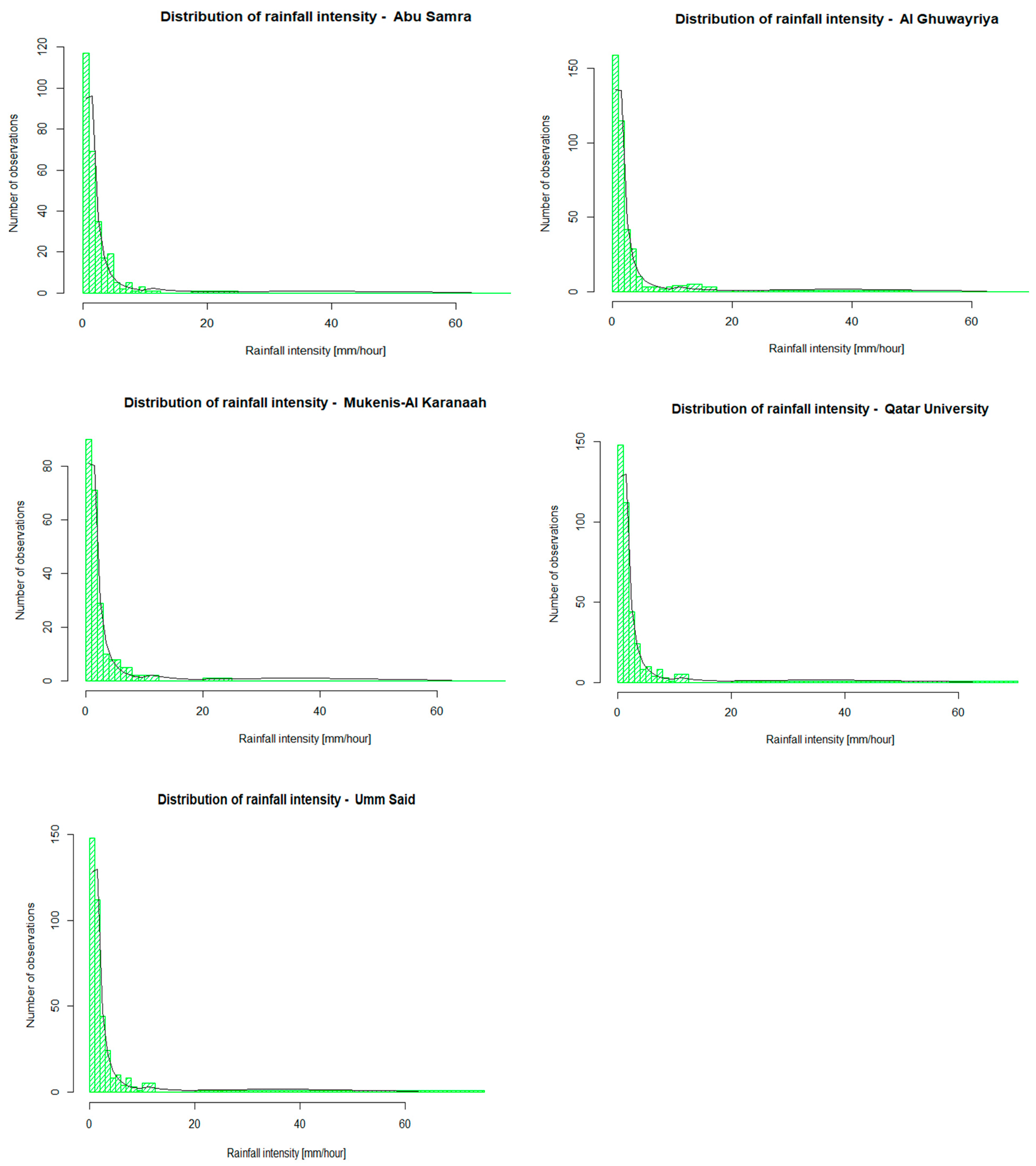
Water 16 01257 g003
Figure 4. Marginal distribution of the rainfall intensity for the five stations: Abu Samra (upper left), Al Ghuwayriya (upper right), Mukenis-Al Karanaah (mid left), Qatar University (mid right), and Umm Said (bottom left). The green curve indicates the observed values as a histogram, and the black line is the theoretically derived marginal distribution.
Water 16 01257 g004
Figure 5. Marginal distribution of the wind speed for the five stations: Abu Samra (upper left), Al Ghuwayriya (upper right), Mukenis-Al Karanaah (mid left), Qatar University (mid right), and Umm Said (bottom left). The green curve indicates the observed values as a histogram, and the black line is the theoretically derived marginal distribution.
Water 16 01257 g005aWater 16 01257 g005b
Figure 6. Marginal distribution of the wind direction for the five stations: Abu Samra (upper left), Al Ghuwayriya (upper right), Mukenis-Al Karanaah (mid left), Qatar University (mid right), and Umm Said (bottom left). The green curve indicates the observed values as a histogram, and the black line is the theoretically derived marginal distribution.
Water 16 01257 g006
Figure 7. Bivariate density function of the wind speed and wind direction based on Bernstein Copula functions shown as 3D-plots for the five stations: Abu Samra (upper left), Al Ghuwayriya (upper right), Mukenis-Al Karanaah (mid left), Qatar University (mid right), and Umm Said (bottom left).
Water 16 01257 g007
Figure 8. Bivariate density function based on Bernstein Copula functions of the wind speed and wind direction, shown as contour plots for the five stations: Abu Samra (upper left), Al Ghuwayriya (upper right), Mukenis-Al Karanaah (mid left), Qatar University (mid right), and Umm Said (bottom left). The orange points are individual observations of wind speed and wind direction. The orange dots are the observations.
Water 16 01257 g008
Figure 9. Bivariate density functions of the rainfall intensity and wind direction based on Bernstein Copula functions shown as 3D plots for the five stations: Abu Samra (upper left), Al Ghuwayriya (upper right), Mukenis-Al Karanaah (mid left), Qatar University (mid right), and Umm Said (bottom left).
Water 16 01257 g009
Figure 10. Bivariate density function based on Bernstein Copula functions of the rainfall intensity and wind direction, shown as contour plots for the five stations: Abu Samra (upper left), Al Ghuwayriya (upper right), Mukenis-Al Karanaah (mid left), Qatar University (mid right), and Umm Said (bottom left). The orange points are individual observations of wind speed and wind direction. The orange dots are observations.
Water 16 01257 g010aWater 16 01257 g010b
Figure 11. Plot of the modeled and observed cumulative probabilities (circles) of ranked normalized observations of the trivariate distribution between rainfall intensity, wind speed, and wind direction. The line indicates where observed values are equal modeled values.
Water 16 01257 g011
Figure 12. Contour plot of the rainfall intensity and wind speed under the condition of a wind direction (upper left) from north (0 degrees) to east (90 degrees), (upper right) from east (90 degrees) to south (180 degrees), (lower left) from south (180 degrees) to west (270 degrees), and (lower right) from west (270 degrees) to north (360 degrees). The orange dots are observations.
Water 16 01257 g012aWater 16 01257 g012b
Figure 13. Positioning of a rain gauge in relation to surrounding objects (WMO [61]).
Water 16 01257 g013
Table 1. Overview of the individual stations used by the study.
Station NameLat (N)Lon IStart DateEnd DatePeriod [Years]QA-Test
Abu Samra24°44′44.78″ N50°49′23.45″ E1 March 200731 March 202316.08Passed
Al Ghuwairiya25°50′26.47″ N51°16′12.22″ E1 January 200931 March 202314.24Passed
Al Wakrah25°11′34.02″ N51°37′8.95″ E1 January 200931 March 202314.24Failed
Mukenis-Al Karanaah25°6′13.41″ N51°10′25.46″ E1 January 200931 March 202314.24Passed
Qatar University25°22′56.34″ N51°28′45.90″ E31 March 200731 March 202316.08Passed
Umm Said24°56′32.34″ N51°34′6.51″ E1 December 200731 March 202315.33Passed
Table 2. Overview of the number of observations at the meteorological stations: The first column also includes dry periods, the second column contains all observations with rainfall, and the third column contains all observations where the rainfall exceeds the threshold of 0.5 mm/h.
Station NameNumber of All ObservationsNumber of Observations with Rainfall Number of Observations with Rainfall Intensity Exceeding the Threshold 0.5 mm/h
Abu Samra141,000524276
Al Ghuwairiya124,872759234
Mukenis-Al Karanaah124,872759233
Qatar University141,0001037370
Umm Said134,400749293
Table 3. Estimated Log Pearson Type III (LP3) density parameters and corresponding p-values and χ2 sums for fitting rainfall intensity distribution.
Station Nameαβγp-ValueΧ2Χ2 Critical (α = 0.05)
Abu Samra2.7950.4766−0.90840.28219.7615.51
Al Ghuwairiya2.3020.5219−0.78510.061014.9115.51
Mukenis Al Karanaa3.1940.4526−1.0230.058913.5915.51
Qatar University2.7980.4766−0.90830.240210.3715.51
Umm Said3.4900.4551−1.0690.069414.5115.51
Average 0.143212.6315.51
Table 4. Estimated GEV density parameters and corresponding p-values and χ2 sums in fitting the wind speed data.
Station Nameξ (Location)α (Scale)k (Shape)p-ValueΧ2Χ2 Critical (α = 0.05)
Abu Samra4.66903.1204−0.08010.92153.2015.51
Al Ghuwairiya3.60532.2580−0.06880.82674.3215.51
Mukenis Al Karanaa3.53191.99800.03520.77404.0515.51
Qatar University2.82141.80820.02880.45247.8115.51
Umm Said3.41991.6947−0.02170.28289.7515.51
Average 0.65155.83
Table 5. Chi-square and p-values for the Mixed von Misses distribution with divisions into 3, 4, 5, and 6 segments to fit wind directional data with 12 bins.
Station NameMvM-3MvM-4MvM-5MvM-6
p-ValueΧ2p-ValueΧ2p-ValueΧ2p-ValueΧ2Χ2 Critical (α = 0.05)
Abu Samra0.7086.320.6856.540.6876.520.8634.6516.92
Al Ghuwairiya0.7226.160.9094.020.8285.070.9143.9616.92
Mukenis Al Karanaa0.9722.780.9662.930.9732.770.9792.5616.92
Qatar University0.5537.810.6117.240.5847.500.8924.2816.92
Umm Said0.4249.140.4249.140.8065.300.8364.9716.92
Average0.6766.440.7195.970.7765.430.8974.08
Table 6. Overview of the estimated MvM-6 distribution parameters at the different stations.
SegmentAbu SamraAl GhuwairiyahMukeynis Al KaranaahQatar UniversityUmm Said
μκwμκwμκwμκwμκw
1−0.41326.04480.4251−1.113118.60380.1557−2.875713.14700.0488−2.845913.23620.0628−1.19380.74050.2802
20.54121.43080.1568−0.23858.60240.1353−1.89182.63540.1169−1.49474.17030.0912−0.14318.43720.3506
31.47430.19040.08890.43951.82210.2865−0.32895.72810.3557−0.66287.12270.34941.01234.02240.1331
41.536130.82430.05901.300677.84440.05880.304353.89370.10770.31547.15360.15931.3267122.04600.0778
51.64810.11020.13711.979427.89850.09680.99016.13510.22021.31134.24330.21981.39673.66990.1188
62.32100.28150.13302.99261.27960.26712.082614.40630.15072.389810.11770.11763.131533.05170.0395
Table 7. Overview of Spearman’s rho correlation, Kendall’s Tau, and Blomqvist’s Beta of the observed wind speed and direction data.
Station NameAbu SamraAl GhuwairiyaMukenis-Al KaranaahQatar UniversityUmm Said
Dep. Structure parameter
Sampled Spearman Rho (ρ)−0.230.05−0.190.060.06
Sampled Kendall’s Tau (τ)−0.170.04−0.130.040.03
Blomqvist Beta (β)−0.220.01−0.20−0.020.04
Table 8. The Spearman Rho, Kendall’s Tau, and Blomqvist Beta for the Bernstein Copula for wind speed and wind direction.
Station NameAbu SamraAl GhuwairiyaMukenis-Al KaranaahQatar UniversityUmm Said
Dep. Structure parameter
BC Spearman Rho (ρ)−0.210.04−0.160.050.05
BC Kendall’s Tau (τ)−0.150.02−0.120.020.03
BC Blomqvist Beta (β)−0.190.02−0.130.030.03
Table 9. Overview of Spearman’s rho correlation, Kendall’s Tau, and Blomqvist’s Beta of the observed rainfall intensity and wind direction data.
Station NameAbu SamraAl GhuwairiyaMukenis-Al KaranaahQatar UniversityUmm Said
Dep. Structure parameter
Sampled Spearman Rho (ρ)0.00−0.02−0.060.020.02
Sampled Kendall’s Tau (τ)0.00−0.02−0.040.010.01
Blomqvist Beta (β)−0.02−0.03−0.06−0.03−0.02
Table 10. The Spearman Rho, Kendall’s Tau, and the Blomqvist Beta for the Bernstein Copula for rainfall intensity and wind direction data.
Station NameAbu SamraAl GhuwairiyaMukenis-Al KaranaahQatar UniversityUmm Said
Dep. Structure parameter
BC Spearman Rho (ρ)0.02−0.03−0.050.010.01
BC Kendall’s Tau (τ)0.00−0.03−0.050.000.01
BC Blomqvist Beta (β)0.01−0.02−0.050.00−0.02
Table 11. The marginal LP3 distribution of the rainfall intensity under the condition of the wind direction for the Qatar University station. The column NEvents indicates how many events are observed for each wind direction shown in the first column.
Direction
(Bearing Degrees)
αβγNEvents
N-E (0–90 degrees)1.8720.690−0.826109
E-S (90–180 degrees)5.6170.278−1.20969
S-W (180–270 degrees)0.9020.960−0.55235
W-N (270–360 degrees)5.4760.314−1.271157
Table 12. The marginal GEV distribution of the rainfall intensity under the condition of the wind direction for the Qatar University station. The column NEvents indicates how many events are observed for each wind direction shown in the first column.
Direction
(Bearing Degrees)
ξ (Location)α (Scale)k (Shape)NEvents
N-E (0–90 degrees)2.9381.850−0.045109
E-S (90–180 degrees)2.9631.873−0.02069
S-W (180–270 degrees)2.4181.5700.22635
W-N (270–360 degrees)2.7641.7740.069157
Table 13. The Joe Copula functions for the bivariate distribution between rainfall intensity and wind speed for a given wind direction.
Direction
(Bearing Degrees)
Preferred CopulaCopula Parameter θBlomqvist βKendall’s τNEvents
N-E (0–90 degrees)Joe Copula1.2940.140.14109
E-S (90–180 degrees)Independent1.0000.000.0069
S-W (180–270 degrees)Independent1.0000.000.0035
W-N (270–360 degrees)Joe Copula1.0830.040.05157
Disclaimer/Publisher’s Note: The statements, opinions and data contained in all publications are solely those of the individual author(s) and contributor(s) and not of MDPI and/or the editor(s). MDPI and/or the editor(s) disclaim responsibility for any injury to people or property resulting from any ideas, methods, instructions or products referred to in the content.

