

On Perturbative Methods for Analyzing Third-Order Forced Van-der Pol Oscillators


1
Department of Mathematical Sciences, College of Science, Princess Nourah bint Abdulrahman University, P.O. Box 84428, Riyadh 11671, Saudi Arabia
2
FIZMAKO Research Group, Department of Mathematics and Statistics, Universidad Nacional de Colombia, Manizales 170001, Colombia
3
Faculty of Engineering and Technology, Future University in Egypt, New Cairo 11835, Egypt
4
Department of Physics, Faculty of Science, Port Said University, Port Said 42521, Egypt
5
Research Center for Physics (RCP), Department of Physics, Faculty of Science and Arts, Al-Mikhwah, Al-Baha University, Al-Baha 1988, Saudi Arabia
*
Author to whom correspondence should be addressed.
Symmetry 2023, 15(1), 89; https://doi.org/10.3390/sym15010089
Submission received: 1 December 2022
/
Revised: 23 December 2022
/
Accepted: 26 December 2022
/
Published: 29 December 2022
(This article belongs to the Special Issue Nonlinear Symmetric Systems and Chaotic Systems in Engineering)
Abstract
:In this investigation, an (un)forced third-order/jerk Van-der Pol oscillatory equation is solved using two perturbative methods called the Krylov–Bogoliúbov–Mitropólsky method and the multiple scales method. Both the first- and second-order approximations for the unforced and forced jerk Van-der Pol oscillatory equations are derived in detail using the proposed methods. Comparative analysis is performed between the analytical approximations using the proposed methods and the numerical approximations using the fourth-order Runge–Kutta scheme. Additionally, the global maximum error to the analytical approximations compared to the Runge–Kutta numerical approximation is estimated.
1. Introduction
The concept of rate of change is central to classical mechanics, particularly in kinematics where all the quantities refer to the extent to which a variable changes with respect to time. In this way the change in position of a body with respect to time defines its speed and, in turn, the change of this quantity with respect to time defines its acceleration. In general in the teaching-learning processes of the movement of bodies, these three concepts (position, velocity and acceleration) are addressed in the vast majority of academic programs. The first approach to the concept of the jerk, denoted as , is a consequence of a rate of change as mentioned above, and corresponds to the change in acceleration with respect to time. In physics and engineering, it is understandable that the jerk is an important concept in the explanation of kinematic phenomena, which occur for example in amusement parks. Because mechanical games produce abrupt changes in the direction and magnitude of the trajectory of the objects moved, the movement is not simple to explain in conventional terms of velocity and acceleration. They involve observing changes in acceleration; therefore, the concept of jerk is very pertinent.
Numerous studies have been conducted on non-linear jerk oscillatory equations [1,2,3,4]. For instance, the dynamics of two different models of jerk oscillators and their applications in telecommunication and electrical engineering have been investigated. The authors used a two-parameter perturbation technique to identify periodic solutions for the two suggested models of jerk oscillators [5]. A linearizing method was carried out to determine the approximate values to the displacement amplitude and frequency for the conservative/non-conservative third-order oscillatory equations [6]. In addition, the fractional Van der Pol–Duffing jerk oscillator was solved using the simplest method without using any perturbative approach [7]. Many other effective methods have been used to solve third-degree oscillatory equations. For example, the harmonic balance method (HBM) was employed for investigating and deriving the lowest-order analytical approximations to some different types of non-linear jerk oscillatory equations [8]. Moreover, a new technique based on classical HBM was implemented to find higher periodic approximations for the different types of non-linear differential equations, including various types of second-order and more-than-second-order derivatives [9]. The multiple scales Lindstedt–Poincare (MSLP) approach was employed to identify approximate analytical solutions to jerk-type equations with cubic non-linearities [10]. Ramos [11] applied approximation techniques to analyze different types of non-linear jerk equations that have analytical periodic solutions. Feng and Chen [12] employed a homotopy analysis technique to identify periodic solutions to a non-linear jerk equation. In addition, an iterative algorithm was applied to find the periods and periodic solutions to non-linear jerk oscillatory equations [13]. He’s homotopy perturbation method (He’s HPM) was applied to solve non-linear jerk oscillatory equations [14]. The authors found that the first-order approximation using He’s HPM produced close matches with the solution using the harmonic balance method. However, in the present investigation, the following different types of third-order non-linear modes/jerk oscillatory equations are considered
Equation (1) is called a jerk oscillatory equation. In our investigation, we are interested in studying the following (un)forced jerk oscillatory equation, which is sometimes called the third-order Van-der Pol (VdP) oscillatory equation
and
The main objectives of this study can be summarized in the following points:
- With respect to the first objective, we seek to find some approximate solutions to Equation (2) using two perturbative methods, known as, the Krylov–Bogoliúbov-Mitropólsky (KBM) method (KBMM) and the multiple scales method (MSM).
- With respect to the second objective, we apply a linear suitable transformation to obtain an approximate solution to the forced jerk oscillatory Equation (3).
- Furthermore, the proposed problem is analyzed numerically via the fourth-order Runge–Kutta (RK4) method. Then, a comparison between the accuracy of all the obtained approximations is considered.
Before starting, let us provide an indication of the suggested methods. Both the KBMM and MSM have been applied for analyzing many second-order oscillatory equations. For instance, Salas et al. [15] used the KBMM for solving coupled damped Duffing oscillators with excited force and to derive some analytical approximations. In addition, the authors compared the KBM approximations and the RK4 numerical approximations. They found that both the analytical and numerical solutions were completely identical, which confirmed the high efficiency of the KBM approximations. Moreover, the KBMM was implemented to find a highly accurate analytic approximation to the generalized VdP oscillatory equation [16]. Both forced and unforced damped/undamped parametric pendulum oscillatory equations were analyzed to obtain approximate solutions using certain effectiveness, and more accurate, analytical and numerical techniques, including He’s frequency-amplitude formulation, He’s HPM, the KBMM, and many others [17]. In addition, a general form to the KBMM was applied for solving a class of weakly non-linear partial differential equations [18]. The MSM was employed for analyzing a class of linear ordinary differential equations (odes) with variable coefficients to find highly accurate solutions [19]. The equation of the VdP oscillator with strong non-linearity was solved using the multiple scales modified Lindstedt–Poincare method and MSM. Then, a convergence criterion for the obtained solutions using the two methods was discussed [20]. Moreover, the modified multiple time scale (MTS) technique was implemented for solving forced vibrational systems with strong non-linearities [21]. The authors [21] only derived the first-order approximation to prevent complexity. Furthermore, the authors proved that the MTS technique was valid for both weakly and strongly non-linear damped forced systems. Based on many published studies, it has been demonstrated that KBMM and MSM are effective and give highly accurate solutions for both weak and strong non-linear oscillatory equations. Motivated by these studies, we focused our investigation on deriving some approximations to the (un)forced jerk oscillatory equation using both KBMM and MSM and compared them with RK4 numerical approximations.
The rest of this paper is structured as follows: In Section 2, a solution to the (un)forced jerk-type oscillatory equation is written in the form of a linear combination consisting of two parts : the first part represents the solution of the unforced jerk-type oscillatory equation in the absence of the excitation force , while the second part appears only if the excitation force is included. The value of the second part is directly derived in this section. However, to find the solution of the unforced jerk-type oscillatory equation , the two suggested perturbative methods (KBMM and MSM) should be considered. The KBMM is used to analyze and derive the second-order approximation to the unforced jerk Van-der Pol oscillatory equation in the first sub-section to Section 2. In the second sub-section to Section 2, the first-order approximation to the unforced jerk Van-der Pol oscillatory equation using the MSM is derived in detail. Finally, the conclusions of our study are presented in Section 3.
2. Methodology of Solution
To analyze the (un)forced jerk oscillatory equation to find some symmetric and highly accurate approximations via KBMM and MSM, we first use the following linear transformation
where for then represents the solution of the i.v.p. (2) or the following initial values problem (i.v.p.) in the absence of the excitation force
while (4) represents the solution of the i.v.p. (3) for . In this case, the value of reads
For example, if we choose
then the following value of is obtained
with
and
where
Now, to find some approximations to the forced jerk oscillatory equation (3), it is sufficient to solve the i.v.p. (5) using the above-mentioned methods and then to insert the value of into solution (4). In the below subsections, we solve the i.v.p. (5) using both KBMM and MSM.
2.1. KBMM for Anatomy Jerk Van-der Pol Oscillatory Equation
The solution to the i.v.p. (5) can be written in the following ansatz form
where the functions and are, respectively, given by
where and and other unknown functions , , , and need to be determined.
Now, by inserting Equations (9) and (10) into , and rearranging the obtained results, we finally get
with
and
Now, by equating to zero the coefficients of ,, and , the following systems are obtained
and
By solving system (12), the values of and are obtained
Using the value of and given in Equation (15) in system (14) and solving the obtained results for zero constant integration, we finally get
and
The following values of and are obtained
with
where the value of is defined in Appendix A and the constants are obtained from the initial conditions (ICs) , and . By inserting Equation (15) into Equation (9), we finally get the second-order KBM analytical approximation to the i.v.p. (5).
2.2. MSM for Anatomy Jerk Van-der Pol Oscillatory Equation
According to the MSM, the first-order approximation to the i.v.p. (5) can be constructed in the following form
or
where and . Here, , , , , , , and are undermined time-dependent functions. We can use relation (20) to find the first-order approximation, while the relation (21) can be used to find the second-order approximation.
In this investigation, we seek to find the first-order approximation to the suggested problem. By substituting solution (20) into , and with the help of the following MATHEMATICA commands,
we get
with
where , and
By solving the system , and , using the following MATHEMATICA commands
we finally get
and
3. Results and Discussion
The second-order KBM analytical approximation (9) and the RK4 numerical approximation are numerically analyzed as illustrated in Figure 1, Figure 2 and Figure 3 for different values of the parameters . In addition, the maximum residual error is estimated according to the following relation
This error is estimated numerically for different values of the parameters , as shown in Table 1. It is observed from both Figure 1, Figure 2 and Figure 3 and Table 1 that there is excellent agreement between both the KBM analytical approximation (9) and the RK4 numerical approximation. Additionally, it is found that the accuracy of the KBM analytical approximation (9) increases with increase in the values of , while has an opposite effect. Moreover, it is noted that the second-order KBM analytical approximation (9) is stable for long time intervals—a feature which may not exist in many other methods.
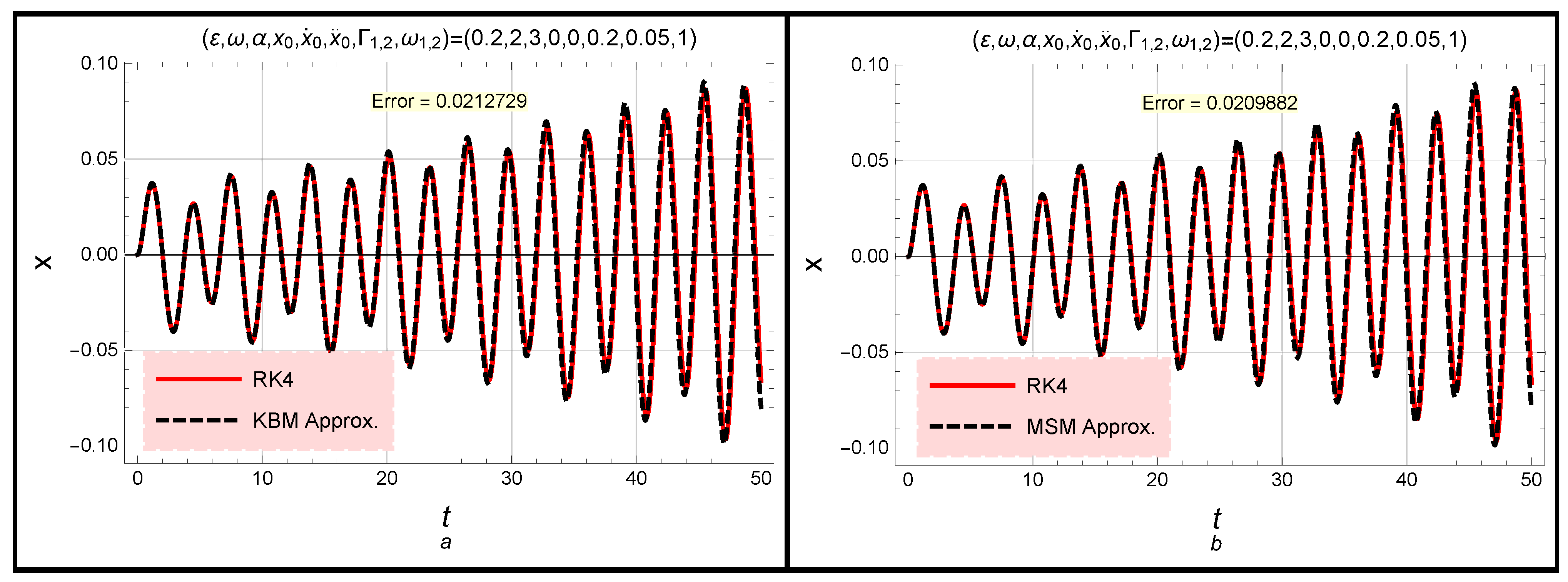
Furthermore, both the second-order KBM analytical approximation (9) and the first-order MSM analytical approximation (20) are compared with the RK4 numerical approximation, as shown in Figure 4a,b for and Figure 4c,d for . It is noted from these figures that there is an almost perfect match between both analytical and numerical solutions, which enhances the accuracy of the solutions obtained. Additionally, it is observed that all the obtained approximations are extremely accurate. Furthermore, the solutions of the forced i.v.p. (3), i.e., , using both the second-order KBM analytical approximation (9) and the first-order MSM analytical approximation (20) with the value of given in Equation (8), are compared with the RK4 numerical approximation, as demonstrated in Figure 5 for . Additionally, the maximum residual error for the second-order KBM analytical approximation (9) and the first-order MSM approximation (20) to the forced i.v.p. (3) are estimated, as shown in Figure 5. It can be seen that the accuracy of the first-order MSM analytical approximation to both the unforced i.v.p. (2) and the forced i.v.p. (3) is better than the second-order KBM analytical approximation. However, both the obtained analytical approximations give satisfactory results and are highly compatible with the RK4 numerical approximations.
4. Conclusions
The third-order/jerk Van-der Pol oscillatory equation has been solved analytically using two perturbative methods, known as, the Krylov–Bogoliúbov-Mitropólsky method (KBMM) and the multiple scales method (MSM). Using the MSM and KBMM, the first- and second-order analytical approximations for both unforced and forced jerk Van-der Pol oscillatory equations have been derived in detail. To investigate the efficiency and the accuracy of all the obtained analytical approximations, a comparison with the RK4 numerical approximations has been reported. In addition, the maximum residual error for all the derived analytical approximations has been estimated. It was found that the accuracy of the first-order MSM analytical approximation was better than the second-order KBM analytical approximation, which means that the second-order MSM analytical approximation will become more accurate than the second-order KBM analytical approximation. However, the two obtained analytical approximations give satisfactory results compared to the RK4 numerical approximations. Thus, we can conclude that the two proposed perturbative methods are effective and accurate for analyzing many non-linear differential equations with higher-order derivatives and higher non-linearities.
Future work: The proposed two perturbative methods can be employed for analyzing the forced jerk oscillatory equation having cosine hyperbolic non-linearity [22].
Author Contributions
Conceptualization, W.A. and E.T.-E.; methodology, A.H.S. and S.A.E.-T.; software, A.H.S. and S.A.E.-T.; validation, W.A., A.H.S. and E.T.-E.; formal analysis, W.A. and S.A.E.-T.; investigation, W.A. and A.H.S.; resources, A.H.S. and S.A.E.-T.; data curation, W.A. and E.T.-E.; writing—original draft preparation, A.H.S. and S.A.E.-T.; writing—review and editing, W.A. and S.A.E.-T.; visualization, W.A. and A.H.S.; supervision, E.T.-E. and S.A.E.-T.; project administration, S.A.E.-T. All authors have read and agreed to the published version of the manuscript.
Funding
The authors express their gratitude to Princess Nourah bint Abdulrahman University Researchers Supporting Project number (PNURSP2023R229), Princess Nourah bint Abdulrahman University, Riyadh, Saudi Arabia.
Institutional Review Board Statement
Not applicable.
Informed Consent Statement
Not applicable.
Data Availability Statement
All data generated or analyzed during this study are included in this published article (More details can be requested from El-Tantawy).
Acknowledgments
The authors are grateful to Princess Nourah bint Abdulrahman University Researchers Supporting Project number (PNURSP2023R229), Princess Nourah bint Abdulrahman University, Riyadh, Saudi Arabia.
Conflicts of Interest
The authors declare that they have no conflict of interest.
Appendix A. The Coefficients of Equation (19)
References
- Gottlieb, H.P.W. Question #38. What is the simplest jerk function that gives chaos? Am. J. Phys. 1996, 64, 525. [Google Scholar]
- Rauch, L.L. Oscillation of a third-order nonlinear autonomous system. In Contributions to the Theory of Nonlinear Oscillations; Lefschetz, S., Ed.; Princeton University Press: Princeton, NJ, USA, 1950; Volume 20, p. 39. [Google Scholar]
- Stirangarajan, H.R.; Dasarathy, B.V. Study of third-order nonlinear systems-variation of parameters approach. J. Sound Vib. 1975, 40, 173. [Google Scholar] [CrossRef]
- Gottlieb, H.P.W. Harmonic balance approach to periodic solutions of non-linear Jerk equations. J. Sound Vib. 2004, 271, 671. [Google Scholar] [CrossRef] [Green Version]
- Kenmogne, F.; Noubissie, S.; Ndombou, G.B.; Tebue, E.T.; Sonna, A.V.; Yemélé, D. Dynamics of two models of driven extended jerk oscillators: Chaotic pulse generations and application in engineering. Chaos Solitons Fractals 2021, 152, 111291. [Google Scholar] [CrossRef]
- El-Dib, Y.O. The simplest approach to solving the cubic nonlinear jerk oscillator with the non-perturbative method. Math. Methods Appl. Sci. 2022, 45, 5165. [Google Scholar] [CrossRef]
- El-Dib, Y.O. An Efficient Approach to solving fractional Van der Pol–Duffing jerk oscillator. Commun. Theor. Phys. 2022, 74, 105006. [Google Scholar] [CrossRef]
- Gottlieb, H.P.W. Harmonic balance approach to limit cycles for nonlinear Jerk equations. J. Sound Vib. 2006, 297, 243. [Google Scholar] [CrossRef] [Green Version]
- Alam, M.S.; Haque, M.E.; Hossain, M.B. A new analytical technique to find periodic solutions of non-linear systems. Int. J. Non-Linear Mech. 2007, 42, 1035. [Google Scholar] [CrossRef]
- Karahan, M.M.F. Approximate Solutions for the Nonlinear Third-Order Ordinary Differential Equations. Z. Naturforsch. 2017, 72, 547. [Google Scholar] [CrossRef]
- Ramos, J.I. Approximate methods based on order reduction for the periodic solutions of nonlinear third-order ordinary differential equations. Appl. Math. Comput. 2010, 215, 4304. [Google Scholar] [CrossRef]
- Feng, S.-D.; Chen, L.-Q. Homotopy Analysis Approach to Periodic Solutions of a Nonlinear Jerk Equation. Chin. Phys. Lett. 2009, 26, 124501. [Google Scholar]
- Liu, C.-S.; Chang, J.-R. The periods and periodic solutions of nonlinear jerk equations solved by an iterative algorithm based on a shape function method. Appl. Math. Lett. 2020, 102, 10615. [Google Scholar] [CrossRef]
- Ma, X.; Wei, L.; Guo, Z. He’s homotopy perturbation method to periodic solutions of nonlinear jerk equations. J. Sound Vib. 2008, 314, 217. [Google Scholar] [CrossRef]
- Salas, A.H.; Abu Hammad, M.; Alotaibi, B.M.; El-Sherif, L.S.; El-Tantawy, S.A. Analytical and Numerical Approximations to Some Coupled Forced Damped Duffing Oscillators. Symmetry 2022, 14, 2286. [Google Scholar] [CrossRef]
- Alhejaili, W.; Salas, A.H.; El-Tantawy, S.A. Approximate solution to a generalized Van der Pol equation arising in plasma oscillations. AIP Adv. 2022, 12, 105104. [Google Scholar] [CrossRef]
- Alyousef, H.A.; Alharthi, M.R.; Salas, A.H.; El-Tantawy, S.A. Optimal analytical and numerical approximations to the (un)forced (un)damped parametric pendulum oscillator. Commun. Theor. Phys. 2022, 74, 105002. [Google Scholar] [CrossRef]
- Alam, M.S.; Akbar, M.A.; Islam, M.Z. A general form of Krylov–Bogoliubov–Mitropolskii methodfor solving nonlinear partial differential equations. J. Sound Vib. 2005, 285, 173–185. [Google Scholar] [CrossRef]
- Ramnath, R.V.; Sandri, G. A generalized multiple scales approach to a class of linear differential equations. J. Math. Anal. Appl. 1969, 28, 339. [Google Scholar] [CrossRef] [Green Version]
- Kumar, M.; Varshney, P. Numerical Simulation of Van der Pol Equation Using Multiple Scales Modified Lindstedt–Poincare Method. Proc. Natl. Acad. Sci. India Sect. A Phys. 2021, 91, 55–65. [Google Scholar] [CrossRef]
- Razzak, M.A.; Alam, M.Z.; Sharif, M.N. Modified multiple time scale method for solving strongly nonlinear damped forced vibration systems. Results Phys. 2018, 8, 231. [Google Scholar] [CrossRef]
- Rajagopal, K.; Kingni, S.T.; Kuiate, G.F.; Tamba, V.K.; Pham, V.-T. Autonomous Jerk Oscillator with Cosine Hyperbolic Nonlinearity: Analysis, FPGA Implementation, and Synchronization. Adv. Math. 2018, 2018, 7273531. [Google Scholar] [CrossRef]
Figure 1.
The KBM second-order approximation (9) (dashed black curve) and RK4 numerical approximation (solid red curve) to the i.v.p. (2) are plotted against different values of damping parameter : (a) for and (b) for .
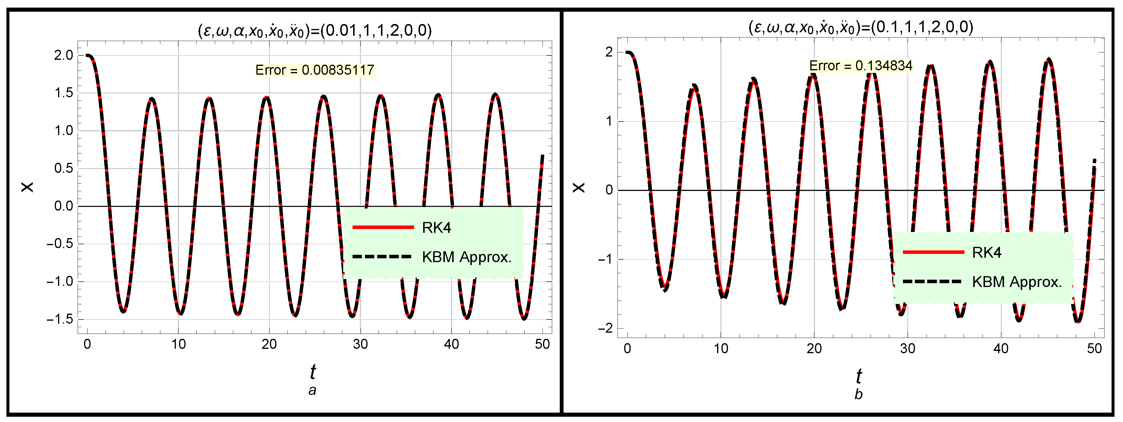
Figure 2.
The KBM second-order approximation (9) (dashed black curve) and RK4 numerical approximation (solid red curve) to the i.v.p. (2) are plotted against different values : (a) for and (b) for .

Figure 3.
The KBM second-order approximation (9) (dashed black curve) and RK4 numerical approximation (solid red curve) to the i.v.p. (2) are plotted against different values of : (a) for and (b) for .

Figure 4.
The KBM second-order approximation (9) (dashed black curve) and RK4 numerical approximation (solid red curve), as well as the MSM first-order approximation (20) (solid red curve) and RK4 numerical approximation (dashed black curve) to the i.v.p. (2), are compared with each other for different values of the damping parameter : (a,b) for and (c,d) for .

Figure 5.
The solution to the forced i.v.p. (3) using (a) the KBM second-order approximation (9) (dashed black curve) and (b) the MSM first-order approximation (20) (dashed black curve) is compared with the RK4 numerical approximation (solid red curve) as for .

Table 1.
The maximum residual error to the second-order KBM analytical approximation (9) is estimated for different values of the parameters .
Table 1.
The maximum residual error to the second-order KBM analytical approximation (9) is estimated for different values of the parameters .
| The Parameter | |
|---|---|
| 0.134834 | |
| 0.00835117 | |
| 0.0368 | |
| 0.0441987 |
Disclaimer/Publisher’s Note: The statements, opinions and data contained in all publications are solely those of the individual author(s) and contributor(s) and not of MDPI and/or the editor(s). MDPI and/or the editor(s) disclaim responsibility for any injury to people or property resulting from any ideas, methods, instructions or products referred to in the content. |
© 2022 by the authors. Licensee MDPI, Basel, Switzerland. This article is an open access article distributed under the terms and conditions of the Creative Commons Attribution (CC BY) license (https://creativecommons.org/licenses/by/4.0/).
Share and Cite
MDPI and ACS Style
Alhejaili, W.; Salas, A.H.; Tag-Eldin, E.; El-Tantawy, S.A. On Perturbative Methods for Analyzing Third-Order Forced Van-der Pol Oscillators. Symmetry 2023, 15, 89. https://doi.org/10.3390/sym15010089
AMA Style
Alhejaili W, Salas AH, Tag-Eldin E, El-Tantawy SA. On Perturbative Methods for Analyzing Third-Order Forced Van-der Pol Oscillators. Symmetry. 2023; 15(1):89. https://doi.org/10.3390/sym15010089
Chicago/Turabian StyleAlhejaili, Weaam, Alvaro H. Salas, Elsayed Tag-Eldin, and Samir A. El-Tantawy. 2023. "On Perturbative Methods for Analyzing Third-Order Forced Van-der Pol Oscillators" Symmetry 15, no. 1: 89. https://doi.org/10.3390/sym15010089
Note that from the first issue of 2016, this journal uses article numbers instead of page numbers. See further details here.